Abstract—The emerging dominance of lean and agile techniques is resulting in a worldwide trend towards shorter product cycles, with smaller lead times and shorter production runs. Simulation is a time-consuming processes and data collection is such a major part of the time period of such a cycle. This paper introduces the circuit of observation concepts which provide a massively reduced cycle time for data collection; this makes it a much more valuable tool in a manufacturing environment and expands its uses due to its greater flexibility. The case study strongly supports the findings.
Index Terms— Activity Sampling, Manufacturing Systems, Simulation.
I. INTRODUCTION
Computer-based simulation is widely used in many disciplines and is becoming an everyday occurrence in the analysis of many fields. Simulation in a manufacturing environment has been used successfully for several decades with its first uses documented in the 1960s. In the paper written by Foster & Rose [1] they discusses various issues that must be overcome in order to spread process modelling of manufacturing systems into mainstream use.
Simulation is closely linked with lean/agile manufacturing [2]. The lean and agile methodologies share many attributes, and agility is considered impossible unless a certain element of leanness exists first. Agile development was first fully discussed in a book by Goldman, Nagel & Preiss [3]. In a manufacturing sense, production must be able to operate over short production runs, with small changeover times and a great degree of flexibility. Song and Nagi et al [4] have identified some of the problems with short-run high variety manufacturing in their development of a modelling system for industrial fabrication shops. This is an extreme example, requiring a specialized modelling tool. Some of the issues this model addresses are encountered in a typical simulation study of a short-run manufacturing facility, such as each product having a unique path to define the process sequence. Short run projects also require additional accuracy due to the lack of data
Manuscript received March 16, 2007.
T. Massey is with Durham University, Durham, U.K.; e-mail: [email protected].
Q. Wang is with Durham University, Durham, U.K. phone: 0044-191-3342381; fax: 0044-191- 3342377; e-mail: [email protected].
available.
As manufacturing cycle times become reduced, there is a reduction in work-in-progress (WIP) and manufacturers seek a faster response, and production runs will operate for less sustained periods of time. The most important aspect of simulation is that it is available for use before it becomes obsolete. In this setting of short production runs and rapid reconstruction, the period of time available to construct accurate simulation models becomes reduced.
II. SIMULATION IN MANUFACTURING SYSTEMS A. The Need for Faster Cycle Times in Simulation Generation
The goal of ‘reducing the period of problem-solving cycles’ is a natural partner of ‘greater acceptance of modelling and simulation within industry’, both goals of the simulation community which were identified by Foster & Rose [1]. In reducing the length of a simulation study by improving the method, the time invested in the process results in more overall value for the effort expended. By improving this ratio of effort to the value of the results gained, it becomes a more attractive process in the manufacturing workplace and its adoption becomes more likely.
B. Shorter Lead Times in Manufacturing
The emergence and dominance of Lean/Agile Manufacturing will in the future produce significantly shorter lead times for products, and rapid change in the manufacturing workplace. Lead times will become shorter and shorter, and more flexible factories result in frequent changes in system. As a simulation becomes redundant when the system is changed, the speed of the generation of the simulation must be proportional to the time the system is in place.
Generating a simulation can be a slow process, particularly for complex systems. Simulation software has progressed significantly in recent years, with graphic interfaces improving the ease of use substantially. While the process of constructing the simulation from the collected data is shortened every day with new software and additional features, this is only the second half of the process. An immense amount of data is required when modelling simulations using this software. Continuous observation is an extremely inefficient process with a significant amount of observation time, in effect, wasted. When recording the required data using continuous observation
Modelling & Simulation of Complex
Manufacturing Systems
to construct a simulation, this ‘dead’ time becomes a significant source of inefficiency in the process.
A method of quickly collecting the data for the simulation is required so that it can reduce the overall time required to produce a simulation. However, a brief read of much of the published literature reveals a significant problem – almost every text on modelling in manufacturing focuses solely on the actual building of the simulation. There is no mention of techniques that can be employed to collect data for the simulation effectively. ‘Discrete Event Simulation: A Practical Approach’ by Pooch & Wall [5] is typical of this attitude. The vast majority of the book focuses on software techniques and applying these, while a sole small chapter entitled ‘Simulation Data Collection’ is written towards the end. The chapter is devoted to collecting data from the simulation, rather than for its construction.
Within the simulation community, it appears that the method of the data collection itself is not something to concern themselves with. This is despite it being an integral part of the process.
III. CIRCUIT OF OBSERVATION
A. Activity Sampling
‘Work Study’ by R.M. Currie [6] discusses a technique which can be used to observe a number of simultaneous processes over a period of time. The method of ‘activity sampling’ considers a continuous process as being comprised of “a number of individual moments during which a particular state of activity or inactivity prevails” [7]. This forms the basis of a technique where a number of individual moments selected at random or fixed intervals can form an estimation of the overall time spent on each activity.
‘Activity Sampling’ is a technique that is “aimed at providing a record of what is actually taking place at the instant the job is observed; it is not a record of what the observer thinks should be happening, nor what has just happened nor is about to happen”[7]. This is an important feature of the technique, as it attempts to provide an objective method of providing a scientific estimation of the percentage of time spent on a given activity, rather than a subjective estimate. Estimations can be formed over a period of time by making observations, to build up a picture of the overall pattern of work.
The technique can be best explained with an example - a single machine, with only two states: active and inactive. Supposing random activity sampling was carried out independently, with thirty random observations over the period, the situation would be as follows:
Number of random observations = 30 Number of non-work observations (*) = 11
Percentage of observations that are non-working = (11/30) x 100 = 36.7%
Therefore, the estimated proportion of non-working time = 36.7%
B. Accuracy
In any sampling activity the estimated value will inevitably differ from the real answer value. With more observations, a more detailed profile would be built up and the accuracy of the estimate would be improved. The accuracy of the figure obtained can be guaranteed to within ± L nineteen times out of twenty (95%), L representing the limits of the permitted variation stated as a percentage of total time. The number of observations (N) required for 95% accuracy to be within the percentage limits, L% is expressed as the given formula:
(1) This can be rewritten as:
(2)
where p is the (approximate) occurrence of the specified activity as a percentage of N. As the number of samples increases, p can be reassessed to give a more accurate value of the 95% variation, L.
C. Circuit of Observation
Activity sampling is used to provide large quantities of data for a relatively low proportion of observation time. It is possible to combine the studies of many different processes into a circuit of observation. A circuit of observation comprises of a set pattern that can be replicated precisely with fixed intervals between each circuit (typically 10 to 15 minutes, depending on the circumstances in each individual case). It can be used to provide data quickly on a number of locations requiring study. Activity sampling is ideal for studying many different operations that occur simultaneously.
A circuit of observation involves making a sample at each location on a circular tour, over a fixed period. Each measurement is made on a circular route that is designed to reduce the time needed to complete the circuit. This allows the maximum amount of data to be made. The observer must establish the locations for which observations are required and adjust the route accordingly.
IV. ADVANTAGES OF ACTIVITY SAMPLING IN SIMULATION A. Study of Multiple Processes Simultaneously
potential data from all the other processes that occur simultaneously. This improves the long-term reliability of the results as data may be recorded over a period of a week, for example, rather than just a day for each process.
There is an issue of activity sampling that it is a sample. In any sampling technique potential for error is introduced. Activity sampling cannot provide the precise values that continuous study can provide, and it is a matter of opinion and the particular circumstances of each case whether this accuracy can be sacrificed for a considerably shorter data collection period.
B. Reduced Chance of Disturbance
Any simulation is concerned with the observation and recreation of a process in its natural state. There are many ways in which observation can disturb how a system acts normally. These include an observer simply becoming an inconvenience, or the act of observation altering behaviour.
A circuit of observation helps to greatly reduce this risk of altering system behaviour as an observer is present for only a very short period of time overall.
C. Collection Period
When similar periods of observation time are invested in both a continuous study and an activity sampling-style study, the activity sampling study will produce results spread over a larger period. This is preferable as it helps to remove the risk of corrupted data produced by random fluctuations or unusual conditions. This should improve the accuracy of the data obtained in its representation of usual conditions.
D. Data Collection Types
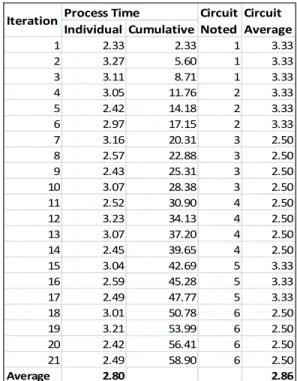
An important part of simulation is the use of process timings or distributions [8]. By recording on each circuit the number of products produced since the last circuit which are awaiting further work, it is possible to form an estimation of the time required by averaging the period by the produced figure for the last interval. Although it does not produce exact timings, over a number of values it should produce an estimation of either the average or distribution. An example of how the averaging works is shown in Table 1.
In Table 1, three items are produced in the first circuit (with duration of 10 minutes). Therefore they are calculated to have an average time each of 3.33 minutes. This process continues with each circuit and, depending on process times, the average over several cycles should imitate the overall average process time. This method can be made more sensitive by shortening the length of time the circuit lasts, however caution should be exercised when reducing the circuit length – a particularly short circuit relative to process length will result in a highly irregular pattern, with several jobs completed one cycle and no jobs completed the next.
Table 1 Example of averaging in circuit of observation
Individual Cumulative
1 2.33 2.33 1 3.33
2 3.27 5.60 1 3.33
3 3.11 8.71 1 3.33
4 3.05 11.76 2 3.33
5 2.42 14.18 2 3.33
6 2.97 17.15 2 3.33
7 3.16 20.31 3 2.50
8 2.57 22.88 3 2.50
9 2.43 25.31 3 2.50
10 3.07 28.38 3 2.50
11 2.52 30.90 4 2.50
12 3.23 34.13 4 2.50
13 3.07 37.20 4 2.50
14 2.45 39.65 4 2.50
15 3.04 42.69 5 3.33
16 2.59 45.28 5 3.33
17 2.49 47.77 5 3.33
18 3.01 50.78 6 2.50
19 3.21 53.99 6 2.50
20 2.42 56.41 6 2.50
21 2.49 58.90 6 2.50
Average 2.80 2.86
Iteration Process Time Circuit Noted
Circuit Average
This method could be extended in certain circumstances to estimate process time distributions, plotting the average times in a histogram. This will require more jobs per cycle to produce a suitable variation of average process times and plot the histogram in any detail, and also more observations to improve its accuracy. With a suitable amount of average times, the histogram can be formed by dividing the average times into groups to form the distribution. This process itself should also improve accuracy, as with even exact process timings they must still be separated into groups to form the distribution. There are some difficulties when calculating average process times from items produced over a time period. It is important that there is a storage bin so that the products can be counted. As processes are part of a flow system, confusion will occur when products are removed for the next process. Either a clear record of products being removed from storage must be available. Alternatively display boards or a similar method display are required to track production, rather than counting a storage bin.
V. METHODOLOGY TESTING –HENDERSON DOORS
The case study at Henderson Doors was intended to establish the general validity of as many as possible of the methods suggested earlier. These included the use of the ‘Circle of Observation’, and an assessment of the ability to map DSM charts directly into the Simul8 application.
A fully mechanised line is used to roll metal doors which are then drilled with holes according to the door design. They are then stored awaiting painting. The painting plant uses a dry powder process that is also highly automated to paint the doors. A complete cycle of the paint plant lasts approximately an hour during which doors are completed coated and then allowed to dry in ovens. After painting, doors are then stored again awaiting final assembly.
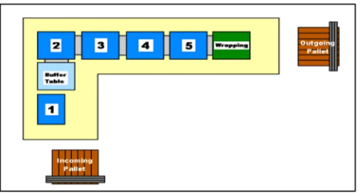
The final assembly line consists of five main work areas as shown in Figure 1, a buffer table before the second area, and a wrapping table for wrapping doors when requested. The stages of the assembly line are outlined below;
Work Area 1 (FA1): Used to fit the external locking points to the door, while door sits vertically.
Buffer Area: Single table with rollers and capacity for one door. Used to lower doors to horizontal position.
Work Area 2 (FA2): Door lowered to horizontal position. Part of the frame is fitted to the door.
Work Area 3 (FA3): Between FA2 to FA5 there is a single continuous roller line for sliding doors along. Further parts of frame/mechanism are fitted in this area.
Work Area 4 (FA4): Door barcode scanned to register completed door. Some final parts are added.
Work Area 5 (FA5): Door rolled onto wrapping table. Door wrapped if required, and then harness looped around door. Door then raised and lifted onto pallet.
Figure 1 Final assembly line
Each workstation is supplied using a kanban system stocked by support staff, and small parts such as screws are supplied from eye-level shelving.
Above the assembly line, two computer monitors display the amount of doors previously produced, split into divisions for each hour. This enables constant feedback to the line on their targets and whether they are being met, and for management to monitor performance easily.
Ideally each workstation (FA1 to 5) would have had a sizeable buffer between each workstation. This would enable the output of each workstation to be monitored for each circuit. The final assembly line was a one-piece-flow line, with each workstation passing work onto the next without a storage stage. This meant that the performance of each workstation could not be monitored simply in terms of items produced, as each workstation worked at effectively the pace of the slowest.
To find a way to estimate the actual work time of each workstation, the utilisation was monitored at each. The utilisation of each workstation was then used to estimate the time spent working on a product as a fraction of the total rate it passed along the assembly line. So if a workstation was working at a rate of 100% overall, its process time would be the same as the products being produced. With only 50% utilisation, then the process time would drop to half the production rate. Overall the production rate in the simulation will be the same, but rather than one ‘process’ block for the whole line, it is split into individual workstations. This is crucial as in the future it is then possible to simulate changing the configuration of the line as well as the number of lines themselves.
It should be noted that the study relates to the actual workstations, rather than the staff at each workstation, so a low utilisation does not relate to the time spent working by staff. It simply reflects that the three teams of staff divide their time between different workstations. By adding the utilisation of all the workstations together, the total is 290% (or 97% per staff team). While this reflects time any work was occurring at that location (so perhaps only one member of staff was actually working rather than both) it generally demonstrates that overall staff utilisation was very high and work was well balanced between teams.
The production figure for each circuit was easily observed from overhead monitors. Each door is barcode scanned at workstation 4 after assembly work, and this is registered on each monitor. This made the production rate for each circuit recorded quickly and without error.
Due to the variety of products passing through the assembly line, it was important to ensure that this was accurately recorded. Initial discussions confirmed that product type could have a significant impact on process times, and therefore would require careful consideration. By examining the outgoing pallet it was possible to note down the recently produced types of product. This also helped to ensure the production figure for the last circuit was correct.
VI. SIMULATIONCONSTRUCTION
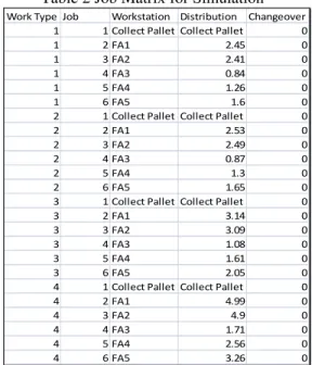
Table 2 Job Matrix for Simulation Work Type Job Workstation Distribution Changeover
1 1 Collect Pallet Collect Pallet 0
1 2 FA1 2.45 0
1 3 FA2 2.41 0
1 4 FA3 0.84 0
1 5 FA4 1.26 0
1 6 FA5 1.6 0
2 1 Collect Pallet Collect Pallet 0
2 2 FA1 2.53 0
2 3 FA2 2.49 0
2 4 FA3 0.87 0
2 5 FA4 1.3 0
2 6 FA5 1.65 0
3 1 Collect Pallet Collect Pallet 0
3 2 FA1 3.14 0
3 3 FA2 3.09 0
3 4 FA3 1.08 0
3 5 FA4 1.61 0
3 6 FA5 2.05 0
4 1 Collect Pallet Collect Pallet 0
4 2 FA1 4.99 0
4 3 FA2 4.9 0
4 4 FA3 1.71 0
4 5 FA4 2.56 0
4 6 FA5 3.26 0
The simulation model as shown in Figure 2 consists of a work centre for each workstation on the line, with process times referencing from the job matrix. The allocation work centre is used to distribute doors according to the percentage distribution of doors to be tested. Although this will not produce the exactly same order of doors in the storage bins (number 1 to 4 for each product type), it will produce the same percentage proportions. The results for each configuration are processed in trial tests of 20 complete runs each time with different random numbers used each time, and results are given as an average over all twenty runs.
The main point of note is the wrapping table area. A proportion of doors are routed to the table for wrapping, while the rest are sent directly on to FA5. This proportion is variable depending on the order, but currently is set at 80.6% which is the percentage of observed doors that were wrapped over the observation period.
Figure 2 Simulation model of final assembly line
VII. SIMULATIONTESTING
This involves setting up a simulation to run using the real life inputs of the system (i.e. in this case the product distribution by percentage and the working time) and studying the output and comparing it with the real-life result. The results of this process are shown below in Table 3
Table 3 Comparisons of real result and simulation result
Each test involved setting the run time of the test in working minutes (length of the day in minutes removing minutes spent on breaks), and the percentage of doors in each category. A trial of twenty runs was then run, with the result being an average of the doors produced over each of the runs. Running each individual test is completed using different random numbers in the simulation package. The alteration of random numbers essentially changes the ‘random behaviour’ of the simulation at any given point, so it is important that multiple trials are run to give a good overall perspective of the system’s performance.
The simulation produces an error on average of just over 7 percent on average. The most significant error (over 10%) is marked as red on the table. These certain days experienced unusual conditions that led to variation in performance. Over the observed period, there was an uneven balance in the type of product that was observed through the line. While a significant number of Canopy products (1 & 2) were observed, a very small number of Tracked products were available for observation.
overall in tests with more than 80% canopy products. However, more error is increasingly likely with an increasing number of tracked products, and with 75% canopy products error reaches above 7%. This should be noted in any future investigation results.
VIII. DISCUSSIONS
The circuit of observation technique was observed to drastically reduce observation time, when compared with direct observation techniques. In testing the technique at PC Henderson Doors Ltd, each circuit commenced every ten minutes. Usually after a period of approximately five minutes the circuit was complete, which allowed five minutes for data entry and some preliminary analysis work.
The simulation, which was produced from the data collected, performed admirably when the amount of observation time was a little over six hours. The average error of the simulation was just 2.51%. This is an excellent level of accuracy, considering the low amount of some types of products that were observed (over 95% of observed products in the system were just two variants) and the estimated wide variation of accuracy at a component level in the simulation.
Simulations that can be constructed with such little required observation time are extremely valuable. They remove a significant element of guesswork in early stages planning and decision-making in manufacturing environments.
As the study continued, it was noted that this method of observation sampling and simulation were ideally suited to be used in conjunction with each other. While a sampling system inherently contains a degree of error within it, the simulation itself essentially helps to ‘double-check’ this error. The process of building the simulation of these components, each with their individual error and testing the error of multiple components on a larger scale helps to ensure that the error within the components is balanced by the system’s component error as a whole.
IX. CONCLUSION
There is a great need for a reduction in the time invested in simulation. It improves the value and flexibility of the process. The longer a simulation takes to construct the higher the chance it will suffer from redundancy before it can help solve the problem it was intended to create.
Data collection should be regarded as an integral part of this process, often forming the majority of the time invested in the problem. The natural method of continuous observation is simply inadequate and there is much potential for improvement. The ‘circuit of observation’ method provided a far superior method of data collection, reducing the observation time on a manufacturing line to a mere six hours. From these observations, the model produced was tested and observed to have an average error of just 2.51%. This error figure was not just caused by the short observation time, but it was also increased due to a lack of product variation in the observed period.
Such a model provides an excellent method of problem solving. Multiple scenarios can then be tested using the devised model, and this much reduced cycle time provides a significant improvement in the value of the entire simulation method. Reducing the time required enables the possibility of management being trained and carrying out the simulation, which in turn reduces many of the other problems possible in simulation such as a lack of familiarity with the system. The manufacturing community would find an improved flexible nature in simulation a way to increase its use and spread the method to a wider variety of areas, achieving Foster & Rose’s goal of its use becoming more widespread.
REFERENCES
[1] J. W. Fowler and O. Rose “Grand challenges in modeling and simulation of complex manufacturing systems”, Simulation, Vol.2, No. 9, 2004, pp. 469-476
[2] A. Gunasekaran and Y. Y. Yusuf “Agile manufacturing: a taxonomy of strategic and technological imperatives”, International Journal of
Production Research, Vol. 40, No. 6, 2002, pp. 1357-1385.
[3] S. L. Goldman, R. N. Nagel, K. Preiss, V. N. Reinhold, Agile competitors and virtual organizations – strategies for enriching the customer, American Society of Mechanical Engineers, 1995.
[4] L. G. Song and R. Nagi, “Design and implementation of a virtual information system for agile manufacturing”, IIE Transactions, Vol. 29, No.10, 1997.
[5] U. W. Pooch, and J. A. Wall, Discrete Event Simulation: A Practical
Approach, FL : CRC Press Taylor & Francis Group, 1992.
[6] Currie, R. M. Work study, 4th ed, Pitman Publishing, 1977, pp231-244. [7] Managers-net (2007, March 13). Activity Sampling [Online]. Avalable:
http://www.managers-net.com/activity_sampling.html.