www.geosci-model-dev.net/9/4339/2016/ doi:10.5194/gmd-9-4339-2016
© Author(s) 2016. CC Attribution 3.0 License.
Air quality modelling in the Berlin–Brandenburg region using
WRF-Chem v3.7.1: sensitivity to resolution of model grid
and input data
Friderike Kuik1,2, Axel Lauer3, Galina Churkina1, Hugo A. C. Denier van der Gon4, Daniel Fenner5, Kathleen A. Mar1, and Tim M. Butler1
1Institute for Advanced Sustainability Studies, Potsdam, Germany 2University of Potsdam, Faculty of Science, Potsdam, Germany
3Deutsches Zentrum für Luft- und Raumfahrt (DLR), Institut für Physik der Atmosphäre, Oberpfaffenhofen, Germany 4TNO, Netherlands Organization for Applied Scientific Research, Utrecht, the Netherlands
5Technische Universität Berlin, Faculty VI – Planning Building Environment, Institute of Ecology,
Chair of Climatology, Berlin, Germany
Correspondence to:Friderike Kuik ([email protected])
Received: 15 July 2016 – Published in Geosci. Model Dev. Discuss.: 3 August 2016 Revised: 3 November 2016 – Accepted: 16 November 2016 – Published: 5 December 2016
Abstract. Air pollution is the number one environmental cause of premature deaths in Europe. Despite extensive reg-ulations, air pollution remains a challenge, especially in ur-ban areas. For studying summertime air quality in the Berlin– Brandenburg region of Germany, the Weather Research and Forecasting Model with Chemistry (WRF-Chem) is set up and evaluated against meteorological and air quality obser-vations from monitoring stations as well as from a field cam-paign conducted in 2014. The objective is to assess which resolution and level of detail in the input data is needed for simulating urban background air pollutant concentrations and their spatial distribution in the Berlin–Brandenburg area. The model setup includes three nested domains with horizon-tal resolutions of 15, 3 and 1 km and anthropogenic emissions from the TNO-MACC III inventory. We use RADM2 chem-istry and the MADE/SORGAM aerosol scheme. Three sensi-tivity simulations are conducted updating input parameters to the single-layer urban canopy model based on structural data for Berlin, specifying land use classes on a sub-grid scale (mosaic option) and downscaling the original emissions to a resolution of ca. 1 km×1 km for Berlin based on proxy data
including traffic density and population density. The results show that the model simulates meteorology well, though ur-ban 2 m temperature and urur-ban wind speeds are biased high and nighttime mixing layer height is biased low in the base
run with the settings described above. We show that the sim-ulation of urban meteorology can be improved when speci-fying the input parameters to the urban model, and to a lesser extent when using the mosaic option. On average, ozone is simulated reasonably well, but maximum daily 8 h mean con-centrations are underestimated, which is consistent with the results from previous modelling studies using the RADM2 chemical mechanism. Particulate matter is underestimated, which is partly due to an underestimation of secondary or-ganic aerosols. NOx (NO+NO2) concentrations are
local pollution patterns in the Berlin–Brandenburg region if the urban land use classes, together with the respective input parameters to the urban canopy model, are specified with a higher level of detail and if urban emissions of higher spatial resolution are used.
1 Introduction
Despite extensive regulations, air pollution in Europe re-mains a challenging issue: causing up to 400 000 prema-ture deaths per year in Europe (EEA, 2015), air pollution is the number one environmental cause of premature deaths (OECD, 2012). Especially in urban areas, air pollution is a problem, with 97–98 % of the urban European population (EU-28) exposed to ozone levels higher than 8 h average concentrations of 100 µg m−3, which the World Health
Or-ganisation (WHO) recommends not to be exceeded for the protection of human health, and ca. 90 % of the urban Euro-pean population (EU-28) exposed to PM2.5(particulate
mat-ter with a diamemat-ter smaller than 2.5 µm) levels higher than the WHO-recommended annual mean of 10 µg m−3in 2011–
2013 (EEA, 2016). Similarly, annual and hourly NO2 limit
values are still exceeded, mainly at measurement site close to traffic. In 2013, the European limit value of 40 µg m−3 was exceeded at 13 % of all stations, all of them situated at traffic or urban sites (EEA, 2016). In Berlin, measured NO2
annual means exceeded the European limit value of the an-nual mean at all but three measurement sites close to traffic in 2014 (Berlin Senate Department for Urban Development and the Environment, 2015a). In addition, current controver-sies on NO2 emissions from cars have triggered additional
discussions on NO2in urban areas.
Numerical modelling is an important tool for assessing air quality from global to local scales. Over the last decades, air quality models have been used to understand the processes leading to air pollution as well as to build a basis for poli-cies defining measures to improve air quality. With ing computing capacities, model resolution has been increas-ing, and different types of 3-D regional chemistry transport models are able to resolve relevant processes down to a hori-zontal resolution of ca. 1 km×1 km (Schaap et al., 2015). At
these resolutions, the models can be used to study the atmo-spheric composition in the urban background.
As a basis for modelling work assessing air quality in the Berlin–Brandenburg area, this study evaluates a setup with the online-coupled numerical atmosphere-chemistry model WRF-Chem (chemistry version of the Weather Research and Forecasting model, Skamarock et al., 2008; Fast et al., 2006; Grell et al., 2005). In the setup presented here, WRF-Chem is coupled with a single-layer urban canopy model (Chen et al., 2011; Loridan et al., 2010). We evaluate the model setup with respect to its skill in simulating meteorological conditions and air pollutant concentrations, with a focus on
NOx (NO+NO2), but also evaluating for particulate matter
(PM10, PM2.5) and O3. The skill in simulating air quality in
an online-coupled model is, besides the choice of the chem-ical mechanism, influenced by the prescribed emissions, the model resolution and the skill in reproducing the observed meteorology. The latter depends on the model resolution, on input data, such as land use data, and on parameterisa-tions of the sub-grid-scale processes, such as effects of urban areas on meteorology. The objective of this study is to ad-dress which resolution and level of detail in the input data, including land use, emissions and parameters characterising the urban area, is needed for simulating urban background air pollutant concentrations and their spatial distribution in the Berlin–Brandenburg area. This is done by evaluating the model results of three nested model domains at 15, 3 and 1 km horizontal resolutions as well as three sensitivity sim-ulations, including updating the representations of the urban area within the urban canopy model, taking into account a sub-grid-scale parameterisation of the land use classes, and downscaling the original emission input data from a hori-zontal resolution of ca. 7 to ca. 1 km. In light of the high computational costs of running the model at a 1 km hori-zontal resolution, it is particularly helpful to find out under which conditions using this model resolution can lead to im-proved results compared to coarser resolutions. This can di-rectly help the design of future air quality modelling studies over the Berlin–Brandenburg region and other European ur-ban agglomerations of similar extent.
The WRF-Chem model has been applied and evaluated in different modelling studies over Europe. For example, Tuc-cella et al. (2012) evaluate a European setup at a horizontal resolution of 30 km×30 km. Brunner et al. (2015) and Im
et al. (2015b, a) analyse the performance of several online-coupled models set up for the Air Quality Model Evaluation International Initiative (AQMEII) phase 2. Among the simu-lations for a European domain, there are seven with different setups of WRF-Chem, performed with a horizontal resolu-tion of 23 km×23 km. Commonly reported biases of
the choice of chemical mechanism, and that RADM2 leads to an underestimations of observed ozone concentrations. PM10
is underestimated by WRF-Chem as compared to regional background observations (Im et al., 2015a). Tuccella et al. (2012) also report an underestimation of PM2.5. Both studies
give various reasons for the mismatch in PM model results and observations, including an underestimation of secondary organic species by the aerosol mechanisms applied. Im et al. (2015a) report an overestimation of nighttime NOxin some
models, including WRF-Chem, which they attribute both to a general underestimation of NO2 during low-NOx
condi-tions and to problems in simulating nighttime vertical mix-ing. They report that NO2is underestimated by most models.
WRF-Chem has also been applied at high spatial res-olutions over urban areas, for example, Mexico City (Tie et al., 2007, 2010), Los Angeles (Chen et al., 2013), Santiago (Mena-Carrasco et al., 2012), the Yangtze River Delta (Liao et al., 2014) and Stuttgart (Fallmann et al., 2016). Tie et al. (2007, 2010) have explicitly assessed how the model reso-lution impacts the simulated ozone and ozone precursors in Mexico City and concluded that a resolution of 24 km is not suitable for simulating concentrations of CO, NOxand O3in
the city centre. They suggest a ratio of city size to model res-olution of 6 : 1 and conclude that a horizontal resres-olution of about 6 km is the best balance between model performance and computational time when simulating ozone and precur-sors in Mexico City. Furthermore, they conclude that the model results for ozone are more sensitive to the model reso-lution than to the resoreso-lution of the emission input data. Other studies have shown that increasing the model resolution does not necessarily lead to an improvement in model results, but that it can be beneficial for amplifying the urban signal (e.g. Schaap et al., 2015, and references therein). They empha-sise that it is only useful to go to model resolutions finer than 20 km if model input data, such as land use data and emission data, are also available at similarly high resolutions. Fall-mann et al. (2016) have combined WRF-Chem with RADM2 chemistry and MADE/SORGAM aerosols with a multi-layer urban canopy model for the area of Stuttgart, studying effects of urban heat island mitigation measures on air quality. One of their findings from the model evaluation is an underesti-mation of daytime NO2by up to 60 %, while O3is slightly
overestimated during the day.
In the Berlin–Brandenburg region, there have been re-gional model simulations of particulate matter with an offline chemistry transport model (Beekmann et al., 2007), along with a measurement campaign focusing on particulate matter in 2001/02. Other modelling studies in this region focused on meteorology: Schubert and Grossman-Clarke (2013) as-sessed the impact of different measures on extreme heat events in Berlin. Trusilova et al. (2016) tested different ur-ban parameterisations in the COSMO-CLM model and their impact on air temperature. Jänicke et al. (2016) used the WRF model to dynamically downscale global atmospheric reanalysis data over Berlin to a resolution of 2 km×2 km,
testing combinations of different planetary boundary layer schemes and urban canopy models. They conclude that simu-lated urban–rural as well as intra-urban differences in 2 m air temperature are underestimated and that the more complex urban canopy models did not outperform the simple slab/bulk approach.
To our knowledge, there are no published studies for the Berlin–Brandenburg region simulating chemistry and aerosols with an online-coupled regional chemistry transport model. Furthermore, only few of the above-mentioned stud-ies included an assessment of urban NOxconcentrations. In
light of the recent exceedances of NO2in European urban
ar-eas, including Berlin, this study can contribute to filling this gap and serve as a basis for future modelling studies address-ing NOxin European urban areas.
2 Model setup
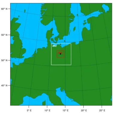
2.1 Model description, chemistry and physics schemes For this study, we use the Weather Research and Forecast-ing model (WRF) version 3.7.1 (Skamarock et al., 2008), with chemistry and aerosols (WRF-Chem, Grell et al., 2005; Fast et al., 2006). We use three one-way nested model do-mains centred around Berlin, at horizontal resolutions of 15 km×15 km, 3 km×3 km and 1 km×1 km (Fig. 1). The
model top is at 50 hPa, using 35 vertical levels. The first model layer is at approximately 30 m above the surface, with 12 levels in the first 3 km. The setup includes the RADM2 chemical mechanism with the Kinetic PreProcessor (KPP) and the MADE/SORGAM aerosol scheme. RADM2 has been used frequently in air quality applications over Europe (e.g. Mar et al., 2016; Im et al., 2015a; Tuccella et al., 2012); the effect of this choice of chemical mechanism on mod-elled concentrations is further discussed in Sect. 4.2. We give the priority to using the KPP solver instead of the QSSA (quasi-steady-state approximation) solver, because Forkel et al. (2015) found that the latter underestimates nighttime ozone titration for areas with high NO emissions. However, this option does not allow us to include the full aqueous-phase chemistry, including aerosol–cloud interactions and wet scavenging, and might thus reduce the model skill in simulating aerosols formed through aqueous-phase reactions as reported in Tuccella et al. (2012). All settings, including the physics schemes used in this study, are listed in Table 1, and the namelist can be found in the Supplement. We use the European Centre for Medium-Range Forecast (ECMWF) In-terim reanalysis (ERA-InIn-terim, Dee et al., 2011) with a hor-izontal resolution of 0.75◦×0.75◦, temporal resolution of
Table 1.Physics and chemistry parameterisation.
Process Scheme Remarks
Cloud microphysics Morrison double-moment
Radiation (short wave) RRTMG called every 15 min Radiation (long wave) RRTMG called every 15 min Boundary layer physics YSU
Urban scheme Single-layer urban canopy model 3 categories: roofs, walls, streets Land surface processes Noah LSM CORINE land use input data Cumulus convection Grell–Freitas switched on for all domains Chemistry RADM2 KPP version (chem_opt=106) Aerosol particles MADE/SORGAM
Photolysis Madronich F-TUV
Figure 1.WRF-Chem model domains with horizontal resolutions of 15 km (d01, outer domain), 3 km (d02, middle domain) and 1 km (d03, inner domain), centred around Berlin, Germany, which is marked black in the figure.
Chemical boundary conditions for trace gases and particulate matter are created from simulations with the global chem-istry transport Model for OZone and Related chemical Trac-ers (MOZART-4/GEOS-5, Emmons et al., 2010).
2.2 Land use specification
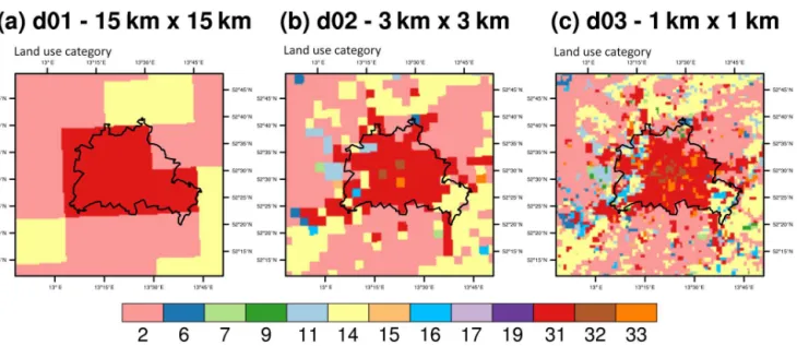
An analysis of the USGS land use data commonly used in WRF showed that the land cover of the region around Berlin is not represented well. In addition, the MODIS land use dataset as implemented in the WRF model from v3.6 only includes one category classifying urban areas. Therefore, we implemented the CORINE dataset (EEA, 2014) to replace the USGS dataset. The original CORINE dataset includes
50 land use classes. The land use classes at the spatial res-olution of 250 m are remapped to 33 USGS land use classes read by WRF, following suggestions of Pineda et al. (2004) (see also Table S1). Additionally, we distinguish between inland water bodies (USGS class 28) and other water bod-ies (USGS class 16). We map the urban land use classes in CORINE to three urban classes used in WRF-Chem, includ-ing “commercial/industry/transport” (USGS class 33), high (USGS class 32) and low (USGS class 31) intensity residen-tial (Tewari et al., 2008), which can be characterised as fol-lows: “low intensity residential” (31) includes areas with a mixture of constructed materials and vegetation. Constructed materials account for 30–80 % of the cover and vegetation may account for 20–70 % of the cover. These areas most commonly include single-family housing units, and popula-tion densities are lower than in high intensity residential ar-eas. “High intensity residential” (32) includes highly devel-oped areas with a high population density. Examples include apartment complexes and row houses. Vegetation accounts for less than 20 % of the area and constructed materials ac-count for 80 to 100 %. Commercial/industrial/transportation (33) includes infrastructure (e.g. roads, railroads) and all highly developed areas not classified as high intensity resi-dential.
Figure 2.CORINE land use classes over Berlin mapped to USGS classes and interpolated to the WRF-Chem grids of(a)15 km,(b)3 km and(c)1 km horizontal resolutions. The classes are the following: 2 – dryland cropland and pasture, 6 – cropland/woodland mosaic, 7 – grassland, 9 – mixed shrubland/grassland, 11 – deciduous broadleaf forest, 14 – evergreen needle leaf forest, 15 – mixed forest, 16 – water bodies, 17 – herbaceous wetland, 19 – barren or sparsely vegetated, 31 – low intensity residential, 32 – high intensity residential, 33 – commercial/industry/transport.
2.3 Urban parameters
We use the single-layer urban canopy model (Kusaka et al., 2001; Kusaka and Kimura, 2004) to account for the modi-fied dynamics by cities, especially Berlin and Potsdam. The urban model takes into account energy and momentum ex-change between urban areas (roofs, walls, streets) and the atmosphere and is coupled to the Noah land surface model. Surface fluxes (heat, moisture) and temperature are calcu-lated as a combination of fluxes from urban and vegetated surfaces, coupled via the urban fraction assigned to the land use type of the grid cell (Chen et al., 2004). We choose to not use a more complex parameterisation of the urban canopy, such as the building effect parameterisation (BEP), because the computational cost is already very high at a horizontal resolution of 1 km×1 km, and a more complex
parameteri-sation of the urban canopy, along with the required increase of vertical model resolution, would increase the computa-tional cost further and require a more detailed input dataset describing the urban structure. Moreover, the BEP is not ap-plicable with the mosaic option in WRF so far and the only applicable planetary boundary layer (PBL) scheme in combi-nation with the BEP and WRF-Chem is the Mellor–Yamada– Janji´c scheme. This scheme often led to stronger biases in simulated 2 m air temperature than other parameterisations such as the YSU scheme (Hu et al., 2010; Loridan et al., 2013; Jänicke et al., 2016), the scheme selected for this study. In addition, Jänicke et al. (2016) could show that the BEP did not outperform simpler approaches such as the bulk scheme or the single-layer urban canopy model with respect to
simu-lating 2 m temperature and that the PBL scheme had stronger influence on simulated 2 m air temperature than the urban canopy parameterisation.
Table 2.Urban parameters for Berlin for the three urban classes low intensity residential (31), high intensity residential (32) and commer-cial/industry/transport (33).
Parameter Default (class 31/32/33) Updated (class 31/32/33)
Roof level (m) 5/7.5/10 3/15/3 Standard deviation of roof height (m) 1/3/4 4.4/6.3/5.2 Roof width (m) 8.3/9.4/10 8.3/16.0/11.8 Road width (m) 8.3/9.4/10 17.5/17.5/17.5 Fraction of urban landscape without 0.5/0.9/0.95 0.4/0.7/0.48 natural vegetation
three urban land use categories. We further update the urban fraction using a spatially more detailed classification of the land use types and the fraction of impervious surface of each area, provided by the Senate Department for Urban Devel-opment and the Environment of Berlin. Following Schubert and Grossman-Clarke (2013), we assume the urban fraction of a grid cell to be equal to the fraction of impervious sur-face. We then define the mean of impervious surface area, weighted by the area of the respective surface within each land use class as the updated urban fraction of the respective class. Following Fallmann et al. (2016) we use the values for thermal conductivity, heat capacity, emissivity and albedo of roofs, walls and streets specified in Salamanca et al. (2012).
2.4 Emissions
For the base run, anthropogenic emissions of CO, NOx,
SO2, non-methane volatile organic compounds (NMVOCs),
PM10, PM2.5 and NH3 are taken from the TNO-MACC III
inventory, with a horizontal resolution of 0.125◦×0.0625◦.
The inventory is based on nationally reported emissions for specific sectors, distributed spatially based on proxy data. In comparison to version II of the inventory (Kuenen et al., 2014), version III includes, amongst other updates, an im-proved distribution of emissions especially around cities. The distribution was improved by no longer using popula-tion density as a default for diffuse (non-point-source) in-dustrial emissions but using inin-dustrial land use as a distribu-tion proxy. Residential solid fuel use (wood, coal) was allo-cated more to rural areas than to large city centres on a per capita basis. Seasonal, weekly and diurnal emission profiles for Germany are applied to the aggregated emissions. This, as well as the speciation of the different NMVOCs, is described in Mar et al. (2016) and von Schneidemesser et al. (2016a). Mar et al. (2016) found that distributing emissions vertically did not strongly impact the model results near the surface. This, along with the low stack height of point sources within Berlin, is why in this study all emissions are released into the first model layer. As much of the NOx emitted within
Berlin is emitted from diesel vehicles (off-road and on-road), which studies have shown to be composed of high propor-tions of NO2(e.g. Alvarez et al., 2008), NOx is emitted as
70 % NO and 30 % NO2(by mole). The latest available
emis-sion dataset is for 2011, which is used in the 2014 simula-tions. Dust, sea salt and biogenic emissions are calculated online, the latter using the Model of Emissions of Gases and Aerosols from Nature (MEGAN v2, Guenther et al., 2006).
We perform a sensitivity simulation for testing the model sensitivity to the spatial resolution of the emission input data (Sect. 2.5). As input to this sensitivity simulation, we downscale the anthropogenic emissions within Berlin onto a grid that is one-seventh of the original resolution, based on two proxy datasets, including traffic densities and pop-ulation (Berlin Senate Department for Urban Development and the Environment, 2011a, b). Traffic densities are used to downscale all emissions from road transport, and population data are used to downscale emissions from industry, residen-tial combustion and product use. Point sources are included in the grid cell within which the point source is located. In the TNO-MACC III inventory, all emissions from the energy industry within Berlin are point sources, and of the point-source emissions from other industry sectors ca. 55 % of the total emissions within Berlin for CO, 9–17 % for particulate matter and up to 1 % for other gases are included as point sources. Agricultural emissions within the city boundaries of Berlin are close to zero, which is why these are used at the original resolution.
2.5 Model simulations
Simulations are done for summer 2014 (31 May–28 August). We chose to simulate the summer of 2014, as this corre-sponds to the time period of the BAERLIN measurement campaign (e.g. Bonn et al., 2016). While mean observed tem-peratures in June and August showed little deviations from the observed 30-year mean (1961–1990) with mean temper-atures of 17.0◦C (June) and 17.2◦C, the July mean
tempera-ture of 21.3◦C was 3.4◦C higher than the 30-year mean.
Pre-cipitation was 12 and 13 % lower than the 30-year mean in June (62.5 mm) and July (60.2 mm), respectively, and it was 48 % lower than the 30-year mean in August, with 33.8 mm (Berlin Senate Department for Urban Development and the Environment, 2014a, b, c).
simulat-ing observed meteorology and atmospheric composition. In addition, sensitivity simulations done for this study are the following, with the changes applied to all three model do-mains of horizontal resolutions of 15, 3 and 1 km:
– S1_urb: updated representation of the urban character-istics of Berlin (see Sect. 2.3 and Table 2);
– S2_mos: consideration of the heterogeneity of the land use categories within one model grid cell (mosaic ap-proach; see Sect. 2.2); and
– S3_emi: using emissions downscaled to ca. 1 km×1 km (see Sect. 2.4).
The purpose of the sensitivity simulations is to assess which resolution and level of detail in the input data, includ-ing land use (S2_mos), emissions (S3_emi) and parameters characterising the urban area (S1_urb), are needed for sim-ulating urban background air pollutant concentrations and their spatial distribution in the Berlin–Brandenburg area, par-ticularly focusing on NOx. We particularly ask whether a
horizontal model resolution of 1 km, together with the above-listed specifications of the input data, leads to model results that differ from those obtained with a horizontal resolution of 3 km.
3 Observational data description and model evaluation procedure
3.1 Data description
In the following, we list the data and data sources that we use for evaluating the present WRF-Chem setup for Berlin and its surroundings. Table 3 gives an overview over all ob-servational data and measurement stations in Berlin and its surroundings used in this study.
3.1.1 DWD stations
We use observations from the German Weather Service (DWD) for the variables of 2 m temperature, 10 m wind speed and direction and precipitation from stations within Berlin and Potsdam for 2014. A second-level quality con-trol, as described in Kaspar et al. (2013), has been applied to the data. Additionally, we obtained mixing layer heights cal-culated from radiosonde observations directly from the DWD at the Lindenberg station south-east of Berlin, as described in Beyrich and Leps (2012). In addition, we use specific humid-ity data from the Global Weather Observation dataset pro-vided by the British Atmospheric Data Centre (BADC) for the same stations.
3.1.2 TU stations
The Chair of Climatology of Technische Universität Berlin (TU) runs an urban climate observation network (Fenner
et al., 2014), from which we use observations of 2 m air tem-perature to complement observations from DWD stations. We include this additional data source, as many of the TU stations are situated in urban built-up areas (see Table 3). We use quality-checked data aggregated to hourly mean values.
3.1.3 GRUAN network
The Global Climate Observing System Upper-Air Network (GRUAN) hosts radiosonde observations at high vertical res-olution, of which we use observations of temperature in Lindenberg (Sommer et al., 2012) to compare them to the modelled profiles. The data used for this study are quality checked, processed and bias corrected as described in Som-mer et al. (2012) and Dirksen et al. (2014).
3.1.4 UBA database and BLUME network
Legally required air quality observations in Germany are re-ported to the Federal Environment Agency (UBA). We use observations of PM10, PM2.5, NO2, NO and O3for 2014
re-ported to UBA. The data are collected from measurement networks operated by the federal states. In Berlin, the offi-cial measurement network is the BLUME network (Berliner Luftgüte-Messnetz), operated by the Senate Department for Urban Development and the Environment of Berlin. In ad-dition to the data reported to the UBA database, we use PM10concentrations measured at three stations in Berlin and
the 2 m temperature measured at the urban built-up station Nansenstraße from the BLUME network.
3.1.5 BAERLIN2014
The BAERLIN2014 (“Berlin Air quality and Ecosytem Re-search: Local and long-range Impact of anthropogenic and Natural hydrocarbons 2014”) campaign took place in Berlin in summer 2014 and is described in detail in Bonn et al. (2016) and von Schneidemesser et al. (2016b). For the present study, we use observations of PM2.5calculated from
particle number concentrations collected near the Nansen-straße station of the BLUME network and observations of the mixing layer height collected at Nansenstraße with a ceilometer. In addition, filter samples taken at Nansenstraße were analysed for the composition of PM10 (von
Schnei-demesser et al., 2016), which we use to compare to simulated aerosols.
3.2 Model evaluation procedure
includ-Table 3.Observational data in Berlin and Potsdam. If one class is given, it refers to the meteorology class if the network is Deutscher Wetterdienst (DWD), Global Climate Observing System Upper-Air Network (GRUAN) or TU, and to the chemistry class otherwise. The abbreviated name (Abbr.) is referred to in tables summarising statistics for the different stations.
Station Abbr. Network Class (meteorology/chemistry) Species used
Nansenstraße nans BAERLIN urban built-up/urban background PM2.5, PM comp., MLH
Nansenstraße nans BLUME urban built-up/urban background NO, NO2, O3, PM10,T2 Amrumer Straße amst BLUME urban background PM10, PM2.5, NO, NO2, O3
Belziger Straße belz BLUME urban background PM10, NO, NO2 Brückenstraße brue BLUME urban background PM10, PM2.5, NO, NO2
J. u. W. Brauer Platz jwbp BLUME urban background NO, NO2
Potsdam-Zentrum pots UBA urban background PM10, PM2.5, NO, NO2, O3
Blankenfelde-Mahlow blan UBA suburban background PM10, PM2.5, NO, NO2, O3
Buch buch BLUME suburban background PM10, NO, NO2, O3 Grunewald grun BLUME suburban background PM10, NO, NO2, O3
Potsdam, Groß Glienicke glie UBA suburban background PM10, NO, NO2, O3 Schichauweg schw BLUME rural industrial NO, NO2, O3
Müggelseedamm mueg BLUME rural background PM10, NO, NO2, O3 Frohnau froh BLUME rural background NO, NO2, O3
Marzahn marz DWD urban built-up T2, prec.,Q2 Botanischer Garten botg DWD/FU urban green T2, prec.,Q2
Tegel tege DWD urban green T2, WS10, WD10, prec.,Q2 Tempelhof temp DWD urban green T2, WS10, WD10, prec.,Q2 Buch buch DWD urban green T2, prec.,Q2
Kaniswall kani DWD rural T2, prec.,Q2
Potsdam pots DWD rural T2, WS10, WD10, prec.,Q2 Schönefeld scho DWD rural T2, WS10, WD10, prec.,Q2 Lindenberg lind DWD/GRUAN rural T, ws,qprofiles
Bamberger Straße bamb TU urban built-up T2 Dessauer Straße dest TU urban built-up T2 Rothenburgstraße roth TU urban built-up T2 Albrechtstraße albr TU urban green T2 Tiergarten tier TU urban green T2 Dahlemer Feld dahf TU rural T2
ing the following diagnostic variables: 2 m temperature (T2), 10 m wind speed and direction (WS10 and WD10), the at-mospheric structure via comparing temperature profiles and mixing layer height (MLH), as well as 2 m specific humidity (Q2) and precipitation. WhileT2, WS10, WD10 and atmo-spheric vertical structure are important parameters for sim-ulating atmospheric chemistry and aerosols,Q2 and precip-itation will not have an impact on our results, as our setup does not include aqueous-phase chemistry or wet scaveng-ing. However, we includeQ2 and precipitation to complete the picture of the evaluation of simulated meteorology as well as to give an indication for future studies based on this setup. Finally, we evaluate the model performance for the main air pollutants including surface O3, NOxand PM, with
a main focus on NOx. We evaluate the model results from all
three domains with horizontal resolutions of 15, 3 and 1 km, which we also refer to as d01, d02 and d03.
3.2.1 Comparison with surface station data
The evaluation of surface parameters is based on statistical metrics including the Pearson correlation coefficient (r), the mean bias (MB) and the normalised mean bias (NMB). The metrics are defined as follows, withnthe number of model– observation pairs,Mthe modelled values,Othe observations andσthe standard deviation of modelled or observed values:
r= 1 (n−1)
n
X
i=1
Mi−M
σM
!
Oi−O
σO
!
MB=1 n
n
X
i=1
Mi−Oi
NMB=
Pn
i=1Mi−Oi
PN i=1Oi
.
scalar and no metrics are calculated for wind direction. The O3, NOxand PM values are calculated from daily averages.
The NMB was only calculated for air pollutants and the mix-ing layer height. For ozone, we also consider the maximum daily 8 h mean (MDA8) concentrations, a metric used in the European Union’s Air Quality Directive.
As an additional means of assessing the model perfor-mance, we look at conditional quantile plots (Carslaw and Ropkins, 2012) for some species. The conditional quantile plot displays the model results, split into evenly spaced bins, in comparison to observations temporally matching the val-ues in the model result bins. Thus, it gives additional insight into how well the modelled values agree with the observa-tions, e.g. on the range of modelled and observed values.
For the comparison between model and observations, we classify the stations in terms of their surroundings, distin-guishing between urban built-up, urban green and rural areas for the meteorology observations, and between urban back-ground, suburban background and rural areas for air quality observations, excluding those from traffic stations.
3.2.2 Evaluation of the atmospheric structure
The mean modelled temperature profiles are compared to observations from radiosondes as follows: as the observed temperatures have a much higher spatial resolution than the model, we select a subset of the observations for compari-son with the model. For every modelled temperature profile at 00:00, 06:00, 12:00 and 18:00 UTC, we select the obser-vations closest to the modelled geopotential height of each model level. The time averaging of modelled geopotential heights is done as follows: we divide the values into verti-cal bins corresponding to the 5th, 10th, 15th percentiles and so on, until the 95th percentile of the modelled geopotential height, and average the temperature as well as the geopoten-tial height over each bin for both model and observations, and over each day of the modelled period. Even though ob-servations of temperature profiles are only available outside of the urban area of Berlin, we include this comparison in order to get a general impression of how the model performs in simulating the vertical atmospheric structure in the lowest 2–3 km.
The modelled MLH is compared to observations in two different ways: firstly, using the planetary boundary layer height directly diagnosed by WRF-Chem, which in the YSU scheme is calculated based on comparing the Richardson number with a critical value of 0 (Hong et al., 2006). Sec-ondly, by calculating the MLH from the simulated profiles of temperature, wind speed and humidity, defining the mixing layer height as the height where the Richardson number is 0.2, following Beyrich and Leps (2012). This corresponds to the method the MLH is derived from using radiosonde ob-servations at Lindenberg.
Figure 3.Comparison of weather types for Berlin calculated from ERA-Interim reanalysis data (top panel) and from WRF-Chem out-put from the domain with 15 km horizontal resolution (bottom panel). Up to three weather types are calculated for each day.
Figure 4.Conditional quantile plot of simulated and observed tem-perature (◦C). The model results are split into evenly spaced bins
Table 4.Statistics of hourly 2 m temperature for JJA for stations, where the land use class of the respective grid cell changes with resolution. “LU” refers to the WRF land use class of the grid cell in the respective domain, “Obs” refers to the JJA observed mean, “Mod” refers to the JJA modelled mean for the respective grid cell. MB is the mean bias for JJA andris the correlation of hourly values. Obs, Mod and MB are in◦C. The statistics are shown for the results from the model domains of 15 km (d01), 3 km (d02) and 1 km (d03) horizontal resolution.
Station Base S1_urb S2_mos
LU Obs Mod MB r Mod MB r Mod MB r
kani d01 31 18.1 19.6 1.5 0.88 19.3 1.2 0.88 19.2 1 0.89 d02 2 18.1 19.4 1.3 0.9 19.3 1.2 0.9 19.3 1.1 0.89 d03 2 18.1 19.4 1.2 0.9 19.2 1.1 0.9 19.2 1.1 0.89 marz d01 2 19.2 18.8 −0.4 0.91 18.7 −0.6 0.9 18.9 −0.4 0.92 d02 31 19.2 19.6 0.4 0.91 19.4 0.2 0.9 19.2 0 0.9 d03 31 19.2 19.7 0.4 0.91 19.3 0.1 0.9 19.2 0 0.9 scho d01 31 18.8 19.6 0.8 0.92 19.3 0.6 0.91 19.2 0.4 0.92 d02 31 18.8 19.9 1.1 0.91 19.7 0.9 0.91 19.4 0.6 0.91 d03 2 18.8 19.3 0.6 0.92 19.2 0.4 0.91 19.3 0.6 0.91 temp d01 31 19.3 19.6 0.3 0.92 19.3 0 0.91 19.3 −0.1 0.92 d02 33 19.3 20.3 0.9 0.9 19.7 0.4 0.9 19.6 0.3 0.9 d03 33 19.3 20.2 0.8 0.9 19.6 0.3 0.9 19.5 0.2 0.9
nans d01 31 20.8 19.6 −1.1 0.91 19.3 −1.4 0.9 19.3 −1.5 0.91 d02 31 20.8 19.9 −0.9 0.9 19.6 −1.1 0.89 19.6 −1.2 0.9 d03 32 20.8 20.2 −0.5 0.9 20 −0.8 0.89 19.6 −1.2 0.9
dahf d01 31 17.9 19.6 1.6 0.88 19.3 1.4 0.89 19.1 1.1 0.9 d02 14 17.9 19.3 1.4 0.9 19.1 1.2 0.9 19.3 1.4 0.88 d03 14 17.9 19.2 1.3 0.9 19 1.1 0.9 19.2 1.3 0.88 bamb d01 31 19.3 19.6 0.4 0.9 19.3 0.1 0.89 19.3 0 0.91 d02 31 19.3 19.9 0.6 0.89 19.6 0.4 0.88 19.6 0.3 0.9 d03 32 19.3 20.2 0.9 0.9 19.9 0.7 0.89 19.5 0.2 0.9
4 Model evaluation results: base run 4.1 Meteorology
Generally, the modelled weather types (see Sect. 3.2) are consistent with those derived from the reanalysis (Fig. 3). Periods in which WRF-Chem weather types disagree with ERA-Interim weather types never exceed two subsequent days and the frequency of WRF-Chem weather types agrees similarly well with ERA-Interim weather types.
The temporal correlation of modelled hourly 2 m tempera-ture with observations is between 0.88 and 0.91 at all stations in and around Berlin and all model domains (Tables 4 and S3 in the Supplement), which shows that the model represents the observed temperature variability well. This is supported by the analysis of the conditional quantiles (Fig. 4), which show that the modelled temperatures match the observations well for a wide range of values. The model is generally bi-ased positively with up to+1.6◦C, though the bias at most
stations is smaller than +1◦C (Tables 4 and S3). In
abso-lute terms, this is within the same range, but never larger than the biases that Trusilova et al. (2016) and Schubert and Grossman-Clarke (2013) found using COSMO-CLM in combination with different urban canopy models for Berlin. Besides, the absolute mean biases are comparable to those
reported by Jänicke et al. (2016), who mainly found negative biases in near-surface air temperature applying WRF 3.6.1 for Berlin and its surroundings, testing two planetary bound-ary layer schemes and three urban canopy models.
The histogram in the conditional quantile plot and the ex-tent of the blue line marking the “perfect model” show that WRF-Chem does not reproduce the highest observed temper-atures. This suggests that the model might have difficulties in simulating pronounced heat wave periods. However, com-paring the modelled daily maximum temperatures to the ob-served daily maximum temperatures (Tables 5 and S4) shows that the bias of the daily maximum temperatures is of a sim-ilar magnitude as the mean bias, with one difference: while the bias of maximum temperatures modelled with 3 and 1 km resolutions is mainly positive, the bias of the maximum tem-peratures modelled with a 15 km resolution is negative. In ab-solute terms, the bias of the daily maximum temperatures is smallest for results obtained with a 1 km resolution, though they only differ very little from the results obtained with a 3 km resolution.
Table 5.Statistics of daily maximum 2 m temperature for JJA for stations, where the land use class of the respective grid cell changes with resolution. “LU” refers to the WRF land use class of the grid cell in the respective domain, “Obs” refers to the JJA observed mean, “Mod” refers to the JJA modelled mean for the respective grid cell. MB is the mean bias for JJA andris the correlation of hourly values. Obs, Mod and MB are in◦C. The statistics are shown for the results from the model domains of 15 km (d01), 3 km (d02) and 1 km (d03) horizontal
resolution.
Station Base S1_urb S2_mos
LU Obs Mod MB r Mod MB r Mod MB r
kani d01 31 24.2 23.8 −0.4 0.88 23.6 −0.6 0.87 23.3 −0.9 0.89 d02 2 24.2 24.4 0.2 0.9 24.3 0.1 0.87 23.9 −0.3 0.9 d03 2 24.2 24.3 0.1 0.9 24.2 0 0.87 23.8 −0.4 0.89 marz d01 2 23.9 23.4 −0.5 0.88 23.2 −0.8 0.86 23 −1 0.9 d02 31 23.9 24.2 0.2 0.89 24 0 0.87 23.5 −0.4 0.9 d03 31 23.9 24.1 0.2 0.89 23.9 0 0.87 23.5 −0.5 0.9 scho d01 31 23.8 23.8 0 0.88 23.6 −0.3 0.87 23.3 −0.5 0.9 d02 31 23.8 24.4 0.6 0.9 24.3 0.5 0.88 23.8 0 0.91 d03 2 23.8 24.3 0.5 0.9 24.1 0.3 0.88 23.7 −0.1 0.9 temp d01 31 24.1 23.8 −0.3 0.88 23.5 −0.6 0.87 23.3 −0.8 0.89 d02 33 24.1 24.5 0.3 0.9 24.3 0.2 0.87 23.8 −0.3 0.9 d03 33 24.1 24.4 0.2 0.9 24.2 0 0.87 23.6 −0.5 0.91
nans d01 31 25.5 23.8 −1.7 0.86 23.5 −1.9 0.85 23.3 −2.2 0.88 d02 31 25.5 24.4 −1.1 0.87 24.2 −1.3 0.85 23.8 −1.7 0.88 d03 32 25.5 24.5 −1 0.87 24.2 −1.3 0.85 23.6 −1.8 0.88
dahf d01 31 23.8 23.7 −0.1 0.89 23.5 −0.3 0.88 23.3 −0.5 0.9 d02 14 23.8 24.1 0.3 0.9 24 0.2 0.88 23.7 −0.1 0.9 d03 14 23.8 24 0.2 0.9 23.8 0 0.88 23.5 −0.3 0.9 bamb d01 31 22.9 23.8 0.9 0.88 23.5 0.7 0.87 23.3 0.4 0.9 d02 31 22.9 24.4 1.5 0.89 24.2 1.3 0.87 23.8 0.9 0.9 d03 32 22.9 24.4 1.5 0.9 24.1 1.2 0.87 23.6 0.7 0.9
generally differ between the 15 and 3 km resolution even if the land use type of both grid cells in which the station is located is the same; the June–July–August (JJA) mean mod-elled temperature only changes by more than 0.1◦C between
the 3 and 1 km resolution if the land use type changes (sta-tions Bamberger Straße, Nansenstraße, Schönefeld). This in-dicates that switching from a horizontal resolution of 15 to 3 km might improve the spatial distribution of modelled tem-peratures, while switching from a horizontal resolution of 3 to 1 km has only a very little effect on improving the model’s skill in simulating the observed temperature, but might be more beneficial if the land use input data are specified with a higher level of accuracy.
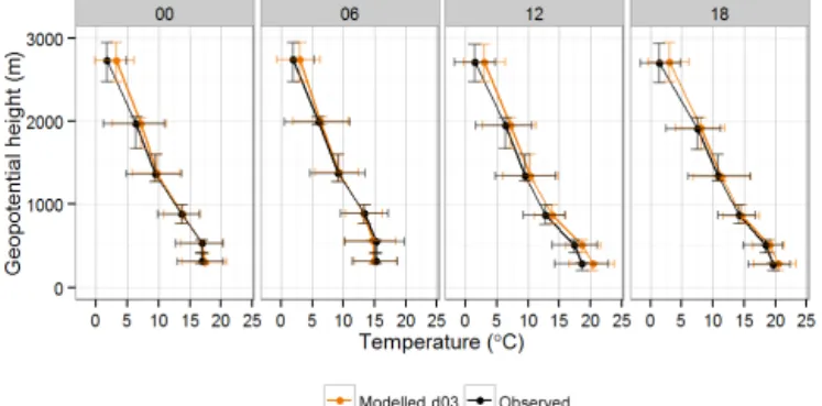
The comparison of simulated with observed temperature profiles (Fig. 5) shows that the model reproduces the ob-served temperature profile well at all times, but that the mod-elled temperature profile at 12:00 UTC is shifted to higher temperatures by ca. 1◦C. The result is similar for all model
resolutions (the profiles for the 15 km and 3 km resolutions can be found in the Supplement in Figs. S1 and S2). In or-der to further evaluate how the present WRF-Chem setup simulates the observed vertical structure, we compare the simulated mixing layer height derived from simulated pro-files of temperature, wind speed and humidity (in the
fol-Figure 5.JJA mean profiles of observed and modelled (base run, 1 km×1 km horizontal resolution) temperature at Lindenberg at 00:00, 06:00, 12:00 and 18:00 UTC. Error bars show the 25th and 75th percentiles of temperature and geopotential height.
Table 6.Statistics of daily minimum, mean and maximum mixing layer height for JJA. “Obs” refers to the JJA observed mean, “Mod” refers to the JJA modelled mean for the respective grid cell. MB is the mean bias for JJA, NMB refers to the normalised mean bias and r is the correlation of hourly values. The values given in the column “YSU” refer to the MLH diagnosed directly by WRF-Chem, while “Calc” refers to the MLH calculated from modelled profiles of temperature, wind speed and humidity. Obs, Mod and MB are given in metres and NMB is given in %. The statistics are shown for the results from the model domains of 15 km (d01), 3 km (d02) and 1 km (d03) horizontal resolution.
Station YSU Calc
Obs Mod MB NMB r Mod MB NMB r
Lindenberg max d01 1414.1 1657.9 243.8 17.2 0.29 1681.8 267.7 18.9 0.28 d02 1414.1 1701.5 287.3 20.3 0.22 1761.1 347 24.5 0.2 d03 1414.1 1635.4 221.3 15.6 0.21 1708.8 294.7 20.8 0.19 mean d01 689.8 736.3 46.6 6.8 0.33 777.2 87.4 12.7 0.27 d02 689.8 718.7 28.9 4.2 0.28 802.8 113 16.4 0.22 d03 689.8 685.7 −4 −0.6 0.27 783.3 93.5 13.6 0.22 min d01 187.5 88.8 −98.7 −52.6 0.09 202.1 14.6 7.8 0.26 d02 187.5 74.4 −113.1 −60.3 0.07 228.8 41.4 22.1 0.27 d03 187.5 75 −112.4 −60 0.17 235.8 48.4 25.8 0.31
Nansenstraße max d01 2312.8 1672.2 1701.4 d02 2312.8 1792.7 1825.8 d03 2312.8 1760.6 1787.2 mean d01 906.7 774 825.6 d02 906.7 785.2 843.9 d03 906.7 741.4 843.7 min d01 175.4 93.7 210.1 d02 175.4 76.9 197.2 d03 175.4 53.1 212.3
depending on model resolution, and the biases of the daily maximum and daily minimum are between +268 m (19 %)
and+347 m (25 %) and between+26 m (14 %) and+48 m
(26 %), respectively (Table 6). There is no consistent trend with increasing model resolution. It is important to note that these results refer to the MLH that we calculated from simu-lated profiles of temperature, wind speed and humidity. How-ever, the MLH diagnosed by the model, in the following also referred to as MLH-YSU, underestimates the observa-tions especially during nighttime (Fig. 6), with a bias of the daily minimum MLH between−99 m (−53 %) and−113 m
(−60 %), or a MLH lower than the calculated one between −128 and−214 %. Differences between the different ways
of deriving the MLH for daily maximum values are less pro-nounced, ranging between 24 m (1 %) and 73 m (4 %). This leads to the conclusion that the model generally simulates the atmospheric structure well, but that the planetary boundary layer scheme underestimates observed MLH during night-time. Similarly, this indicates that the mixing might also be underestimated by the boundary layer scheme during night-time conditions.
Comparing the model results to ceilometer observations from Berlin at the Nansenstraße station also indicates that the diurnal variation is reproduced correctly (Fig. S9 in the Supplement). The comparison of daily minimum MLH with ceilometer observations also shows an underestimation of MLH-YSU in the same range as at Lindenberg. However,
Figure 6.Daily minimum, mean and maximum mixing layer height as observed in Lindenberg, diagnosed by WRF-Chem and calcu-lated from modelled profiles of temperature, wind speed and hu-midity (base run, 1 km×1 km horizontal resolution).
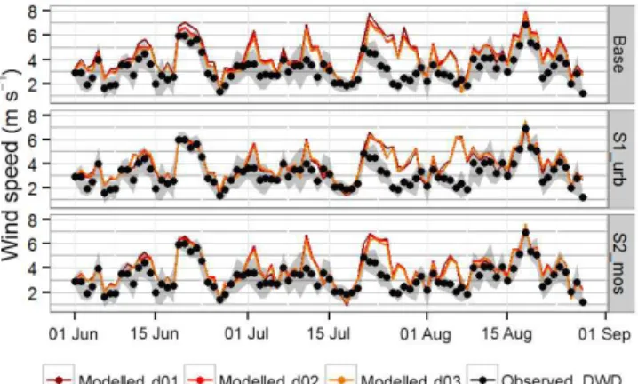
Figure 7.Daily mean observed and modelled wind speed from the base run, S1_urb and S2_mos, for all three model domains (d01 – 15 km horizontal resolution, d02 – 3 km, d03 – 1 km). The figures show means over the daily means of three stations in Berlin (Tegel, Schönefeld and Tempelhof). The grey shades show the variability between the daily means of these stations, corresponding to the 25th and 75th percentiles of the individual stations’ daily means. For the model results, the grid cells corresponding to the location of the stations were extracted.
Simulated hourly wind speed correlates with observations with a correlation coefficient between 0.5 and 0.6 (Table S5 in the Supplement), which is comparable to simulations for the European domain (Mar et al., 2016). Wind speed is over-estimated between 0.4 m s−1 (15 %) and 1.4 m s−1 (50 %), depending on the station. The overestimation is especially strong at stations with mean observed wind speeds below 3 m s−1, as well as for a period of easterly winds in
mid-July (Fig. 7). The most frequently observed wind direction at three stations in Berlin and in Potsdam in June, July and Au-gust 2014 is westerly. This is reproduced by the model, with better skill with increasing resolution (Fig. 8). Depending on the modelled wind direction, the bias in wind speed differs: while the bias (averaged over all four stations) is lower than 1 m s−1for modelled wind from north to south-east, the bias
is larger for wind simulated from east and north-east. In ad-dition, the conditional quantile plot of wind speed, split by modelled wind direction, also shows that the model’s skill in simulating wind speed from west and south-west is higher (see Fig. S3 in the Supplement).
Both the diurnal variability and the magnitude of specific humidity are simulated well by the model, with normalised mean biases between −7 and +7 % and correlation
coeffi-cients of 3-hourly values of around 0.8 (not shown). Precipi-tation is simulated well with the 3 and 1 km horizontal reso-lution: both the number of days with precipitation rates larger than 0.01 mm h−1and the total amount of precipitation in the
simulated period agree well with the observations (Fig. 9). Model results from the 15 km resolution overestimate the number of days with precipitation larger than 0.01 mm h−1
by ca. 30 % and the amount by ca. 50 %. This shows that the
Figure 8.Wind roses over observed and modelled values for JJA, including observations and model results for three stations in Berlin (Tegel, Schönefeld and Tempelhof) and from all three model do-mains (d01 – 15 km horizontal resolution, d02 – 3 km, d03 – 1 km). The bars refer to the frequency of how often wind was coming from the respective direction and the colours indicate how often the wind speed was observed or modelled in the indicated interval.
Figure 9. (a)Station average (mean) precipitation sum of observa-tions and model results (base run),(b)median number of days with precipitation observed or modelled. A day is counted if observed or modelled precipitation was more than 1 mm h−1. Ranges indicate
the variability between the different stations. Both panels(a)and (b)show averages over nine stations and the corresponding model grid cells in Berlin and its surroundings. Model results are given for all three model domains (d01 – 15 km horizontal resolution, d02 – 3 km, d03 – 1 km).
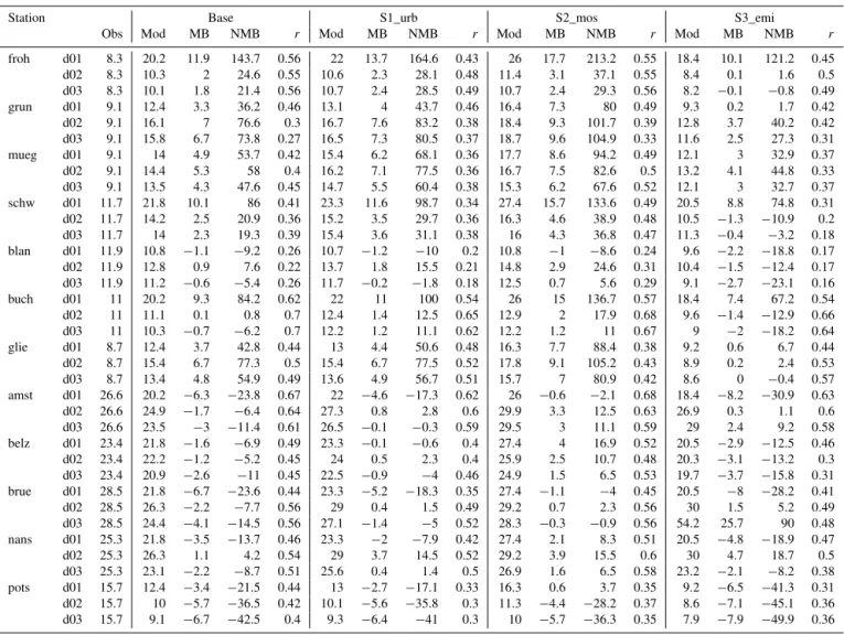
Table 7.Statistics of daily NOxfor JJA. “Obs” refers to the JJA observed mean, “mod” refers to the JJA modelled mean for the respective
grid cell. MB is the mean bias for JJA, NMB refers to the normalised mean bias and r is the correlation of hourly values. Obs, Mod and MB are given in µg m−3and NMB is given in %. The statistics are shown for the results from the model domains of 15 km (d01), 3 km (d02) and 1 km (d03) horizontal resolution.
Station Base S1_urb S2_mos S3_emi
Obs Mod MB NMB r Mod MB NMB r Mod MB NMB r Mod MB NMB r
froh d01 8.3 20.2 11.9 143.7 0.56 22 13.7 164.6 0.43 26 17.7 213.2 0.55 18.4 10.1 121.2 0.45
d02 8.3 10.3 2 24.6 0.55 10.6 2.3 28.1 0.48 11.4 3.1 37.1 0.55 8.4 0.1 1.6 0.5
d03 8.3 10.1 1.8 21.4 0.56 10.7 2.4 28.5 0.49 10.7 2.4 29.3 0.56 8.2 −0.1 −0.8 0.49
grun d01 9.1 12.4 3.3 36.2 0.46 13.1 4 43.7 0.46 16.4 7.3 80 0.49 9.3 0.2 1.7 0.42
d02 9.1 16.1 7 76.6 0.3 16.7 7.6 83.2 0.38 18.4 9.3 101.7 0.39 12.8 3.7 40.2 0.42
d03 9.1 15.8 6.7 73.8 0.27 16.5 7.3 80.5 0.37 18.7 9.6 104.9 0.33 11.6 2.5 27.3 0.31
mueg d01 9.1 14 4.9 53.7 0.42 15.4 6.2 68.1 0.36 17.7 8.6 94.2 0.49 12.1 3 32.9 0.37
d02 9.1 14.4 5.3 58 0.4 16.2 7.1 77.5 0.36 16.7 7.5 82.6 0.5 13.2 4.1 44.8 0.33
d03 9.1 13.5 4.3 47.6 0.45 14.7 5.5 60.4 0.38 15.3 6.2 67.6 0.52 12.1 3 32.7 0.37
schw d01 11.7 21.8 10.1 86 0.41 23.3 11.6 98.7 0.34 27.4 15.7 133.6 0.49 20.5 8.8 74.8 0.31
d02 11.7 14.2 2.5 20.9 0.36 15.2 3.5 29.7 0.36 16.3 4.6 38.9 0.48 10.5 −1.3 −10.9 0.2
d03 11.7 14 2.3 19.3 0.39 15.4 3.6 31.1 0.38 16 4.3 36.8 0.47 11.3 −0.4 −3.2 0.18
blan d01 11.9 10.8 −1.1 −9.2 0.26 10.7 −1.2 −10 0.2 10.8 −1 −8.6 0.24 9.6 −2.2 −18.8 0.17
d02 11.9 12.8 0.9 7.6 0.22 13.7 1.8 15.5 0.21 14.8 2.9 24.6 0.31 10.4 −1.5 −12.4 0.17 d03 11.9 11.2 −0.6 −5.4 0.26 11.7 −0.2 −1.8 0.18 12.5 0.7 5.6 0.29 9.1 −2.7 −23.1 0.16
buch d01 11 20.2 9.3 84.2 0.62 22 11 100 0.54 26 15 136.7 0.57 18.4 7.4 67.2 0.54
d02 11 11.1 0.1 0.8 0.7 12.4 1.4 12.5 0.65 12.9 2 17.9 0.68 9.6 −1.4 −12.9 0.66
d03 11 10.3 −0.7 −6.2 0.7 12.2 1.2 11.1 0.62 12.2 1.2 11 0.67 9 −2 −18.2 0.64
glie d01 8.7 12.4 3.7 42.8 0.44 13 4.4 50.6 0.48 16.3 7.7 88.4 0.38 9.2 0.6 6.7 0.44
d02 8.7 15.4 6.7 77.3 0.5 15.4 6.7 77.5 0.52 17.8 9.1 105.2 0.43 8.9 0.2 2.4 0.53
d03 8.7 13.4 4.8 54.9 0.49 13.6 4.9 56.7 0.51 15.7 7 80.9 0.42 8.6 0 −0.4 0.57
amst d01 26.6 20.2 −6.3 −23.8 0.67 22 −4.6 −17.3 0.62 26 −0.6 −2.1 0.68 18.4 −8.2 −30.9 0.63
d02 26.6 24.9 −1.7 −6.4 0.64 27.3 0.8 2.8 0.6 29.9 3.3 12.5 0.63 26.9 0.3 1.1 0.6
d03 26.6 23.5 −3 −11.4 0.61 26.5 −0.1 −0.3 0.59 29.5 3 11.1 0.59 29 2.4 9.2 0.58
belz d01 23.4 21.8 −1.6 −6.9 0.49 23.3 −0.1 −0.6 0.4 27.4 4 16.9 0.52 20.5 −2.9 −12.5 0.46
d02 23.4 22.2 −1.2 −5.2 0.45 24 0.5 2.3 0.4 25.9 2.5 10.7 0.48 20.3 −3.1 −13.2 0.3
d03 23.4 20.9 −2.6 −11 0.45 22.5 −0.9 −4 0.46 24.9 1.5 6.5 0.53 19.7 −3.7 −15.8 0.31 brue d01 28.5 21.8 −6.7 −23.6 0.44 23.3 −5.2 −18.3 0.35 27.4 −1.1 −4 0.45 20.5 −8 −28.2 0.41
d02 28.5 26.3 −2.2 −7.7 0.56 29 0.4 1.5 0.49 29.2 0.7 2.3 0.56 30 1.5 5.2 0.49
d03 28.5 24.4 −4.1 −14.5 0.56 27.1 −1.4 −5 0.52 28.3 −0.3 −0.9 0.56 54.2 25.7 90 0.48 nans d01 25.3 21.8 −3.5 −13.7 0.46 23.3 −2 −7.9 0.42 27.4 2.1 8.3 0.51 20.5 −4.8 −18.9 0.47
d02 25.3 26.3 1.1 4.2 0.54 29 3.7 14.5 0.52 29.2 3.9 15.5 0.6 30 4.7 18.7 0.5
d03 25.3 23.1 −2.2 −8.7 0.51 25.6 0.4 1.4 0.5 26.9 1.6 6.5 0.58 23.2 −2.1 −8.2 0.38
pots d01 15.7 12.4 −3.4 −21.5 0.44 13 −2.7 −17.1 0.33 16.3 0.6 3.7 0.35 9.2 −6.5 −41.3 0.31 d02 15.7 10 −5.7 −36.5 0.42 10.1 −5.6 −35.8 0.3 11.3 −4.4 −28.2 0.37 8.6 −7.1 −45.1 0.36
d03 15.7 9.1 −6.7 −42.5 0.4 9.3 −6.4 −41 0.3 10 −5.7 −36.3 0.35 7.9 −7.9 −49.9 0.36
4.2 Chemistry and aerosols 4.2.1 Nitrogen oxides and ozone
The mean bias of modelled NOxdepends on the type of
ob-servations that it is compared with (Table 7): for rural sites close to Berlin and Potsdam, it is biased positively. Modelled NOx at urban background sites is mainly biased negatively,
while the bias is positive or negative at suburban background sites. The maximum bias of all sites (Table 7) is improved with increasing spatial resolution from 15 to 3 km, from
+11.9 to +5.3 µg m−3 (rural), +9.3 to +6.7 µg m−3
(sub-urban background) and −6.7 to −5.7 µg m−3 (urban
back-ground). This indicates that generally a horizontal resolution of 3 km is better suited to resolve the spatial NOx patterns
within a city of the size of Berlin even with emission input data coarser than 3 km, which is in line with the results of Tie et al. (2010) for Mexico City. A 15 km resolution is not
suffi-cient to resolve the differences between rural and urban con-centrations (Fig. 10). Comparing the mean bias between the 3 and 1 km resolutions further shows that, with an emission inventory of 7 km horizontal resolution, the 1 km resolution does not generally improve the results.
As a first step for model-based assessments of urban NOx
concentrations, it is important to be able to simulate daily maximum urban background NOxconcentrations well. In
or-der to assess the model’s skill in reproducing these concen-trations, we compare modelled diurnal cycles of NOx to
ob-served diurnal cycles (Fig. 11). The comparison shows that the WRF-Chem setup presented here is not able to simulate the observed diurnal cycle at any of the three resolutions, overestimating NOxconcentrations during nighttime and
night-(a) Base
(b) S1_urb
(c) S2_mos
(d) S3_emi
NO
xconcentration (µg m
-3)
Figure 10.JJA mean modelled (coloured fields) and observed (coloured circles) NOx concentration in Berlin and its surroundings from
(a)the base run,(b)S1_urb,(c)S2_mos and(d)S3_emi. The left column shows results obtained with the 15 km horizontal resolution, the middle shows results from a 3 km horizontal resolution and the right column shows results from a 1 km horizontal resolution.
time overestimation is likely the model’s underestimation of nighttime mixing as discussed above. This is supported by the vertical distribution of NOxat several locations in the
ur-ban area, which shows a strong gradient between the first and second model layer (e.g. Fig. S10 in the Supplement as an ex-ample). A contribution to the daytime underestimation might be uncertainties in the emission inventory: while the share of traffic NOxemissions to total NOxemissions within Berlin is
just above 35 % in the TNO-MACC III inventory, estimates from the Berlin Senate range around 40–45 % for 2008 and 2009 (Berlin Senate Department for Urban Development and
the Environment, 2015b). Using an up-to-date bottom-up lo-cal inventory might contribute to correcting this bias. We can exclude the diurnal cycle applied to the traffic emissions as a reason for the underestimation of the traffic peak in the morning hours – comparing it to diurnal cycles calculated from traffic counts in Berlin shows a good agreement (Fig. S8 in the Supplement). An additional source of bias might be the chemical mechanism itself: in box model studies, Knote et al. (2015) compared different chemical mechanisms and found a difference in simulated summertime NOx of up to
Figure 11. Mean diurnal cycles of NO, NO2, NOx and O3 for
all Berlin and Potsdam urban background stations as observed and modelled by the base run, S1_urb, S2_mos and S3_emi. Model re-sults are given for all three model domains (d01 – 15 km horizontal resolution, d02 – 3 km, d03 – 1 km). The diurnal cycle is averaged over six stations for NO, NO2and NOxand three stations of O3.
The grey shaded areas represent the variability between the differ-ent stations’ diurnal cycles, showing the 25th and 75th percdiffer-entiles.
the multi-mechanism mean was only of the order of a few per cent for summertime conditions simulated with RADM2, which is the mechanism used in this study. A further reason for the model bias might also be the principal challenge of comparing grid cell averages with point observations, par-ticularly in regions with a high variability on small spatial scales, which is quite typical for cities. Regarding the rela-tively coarse vertical resolution of the model, extrapolation from the first model level to the surface (e.g. Simpson et al., 2012) might allow for a better comparability between model and observation. The spatial representativeness of a measure-ment site for a larger area such as the 1 km×1 km grid cells,
however, might be somewhat limited particularly for urban background sites, which can be influenced by local sources and sub-grid-scale variations in emissions that cannot be cap-tured with WRF-Chem.
Additionally, we compare the simulated NO and NO2to
observations as described in Sect. 3.1 (Figs. 11, S6, S7 and Tables S6, S7 in the Supplement). As for NOx, the bias of
modelled NO depends on the station type. For suburban and urban background stations, NO is on average mainly biased negatively up to−2.5 µg m−3(−60 %), while it shows a
pos-itive bias at some of the rural stations. Part of this negative bias is due to a lower detection limit in the observation data ranging between 0.1 and 2 µg m−3depending on the station.
While this is not the main contribution to the bias in NOx, it
does play a larger role when only looking at NO, as for some of the stations a large share of the observed hourly values lies at or below this threshold both in the observed and modelled data (up to 94 %). The diurnal cycle of NO is modelled in
good agreement with the observations, but the peak values are underestimated (Fig. 11). Especially for urban sites, the bias is larger when simulated with a 15 km resolution than with 3 and 1 km resolutions. Modelled NO2 is on average
mostly biased high, with up to 11.1, 5.3 and 4.5 µg m−3for
rural sites and up to 10.2, 7.3 and 6.5 µg m−3 for suburban
sites (15, 3 and 1 km resolution). Urban background sites are both biased high and low. It is important to note that the pos-itive bias always results from overestimations during night-time, while daytime NO2, as total NOx, is always biased low,
though with a smaller daytime bias for suburban and rural sites than for the urban background. These results are in line with what has been discussed for NOx above and indicate
that, in addition to the model resolution, the resolution of emissions might play an important role for simulating day-time NOx concentrations in cities, as more NOx is emitted
near streets than at the edges of the city, which can hardly be captured with emission input data of a horizontal resolution of 7 km.
O3daily means and especially MDA8 ozone are
underes-timated by the model (Fig. 11 and Table S8), with biases of up to ca.−10 µg m−3(mean) and−13 µg m−3(MDA8). This
is consistent with what has been reported for a coarse Eu-ropean domain using RADM2 chemistry (Mar et al., 2016) and in line with previous studies showing a deficiency of many online-coupled models, including WRF-Chem with the RADM2 chemical mechanism, in simulating peak ozone concentrations (e.g. Im et al., 2015a). Mar et al. (2016) sug-gested that the low bias in modelled ozone could be par-tially explained by the inorganic rate coefficients used in the RADM2 mechanism. Furthermore, it is in line with studies identifying the choice of chemical mechanism as a reason for differences in simulated ozone concentrations (e.g. Coates and Butler, 2015; Knote et al., 2015). The choice of chemi-cal mechanism, but not so much the modelled meteorology being an important cause of this bias is further supported by the fact that maximum temperatures are generally simulated well by the model, and MDA8 ozone is underestimated even when daily maximum temperatures are simulated correctly. The mean O3is still simulated reasonably well, though the
model underestimates at night and overestimates during the morning hours. The bias is consistent with a bias in NOx
diurnal cycles discussed above: in particular, the underesti-mation of O3during nighttime is consistent with an
overes-timation of NOx; the overestimation of O3 in the morning
hours might result from too much NO2accumulating at the
surface, which is photolysed when the sun rises.
4.2.2 Particulate matter
The mean bias of the simulated PM10 amounts to −50 %
(Fig. 12 and Table S9 in the Supplement), which is relatively consistent at all eight stations within and around Berlin as well as at all three model resolutions. Modelled PM2.5
Figure 12.Daily mean PM10and PM2.5concentrations as observed
and modelled (base run) at urban background stations in Berlin. Daily means are averaged over five stations for PM10and four
sta-tions for PM2.5. The grey shaded areas represent the variability
between the different stations, showing 25th and 75th percentiles. Model results are given for all three model domains (d01 – 15 km horizontal resolution, d02 – 3 km, d03 – 1 km).
Table S10 in the Supplement). From previous studies with the MADE/SORGAM aerosol scheme it is known that it un-derestimates the secondary organic aerosol contribution to PM (Ahmadov et al., 2012). Comparing the JJA-averaged model output to components of PM10 observed at
Nansen-straße during the BAERLIN2014 campaign is in line with these results: while the observations show a mean concen-tration of organic carbon of 5.6 µg m−3, the modelled par-ticulate organic matter, including organic carbon, is on aver-age 0.8 µg m−3. In addition, the comparison shows that the
contribution of black carbon (BC) to PM might be under-estimated, with observed elemental carbon (EC) concentra-tions of 1.4 µg m−3on average and mean modelled BC
con-centrations of 0.2 µg m−3, though the modelled value is still
within the range of observed values in individual samples. The underestimation of organic carbon (OC) and, to a lesser extent, BC being causes of the underestimation of PM10 is
supported by the fact that, on average, model results compare reasonably well with the observations of other components of PM10: modelled sulfate, nitrate and ammonium amounts to
1.8, 0.5 and 0.7 µg m−3, while the mean observed concentra-tions are 1.9, 0.9 and 0.6 µg m−3. Modelled sea salt amounts to 1.0 µg m−3, and observed sodium and chloride are 0.5 and 0.6 µg m−3, respectively. An additional underestimation of
mineral dust or re-suspended road dust emissions, such as brake and tyre wear, primarily contributing to PM10, might
explain why PM10is underestimated more than PM2.5. As for
the simulated chemical species, part of the bias might be due to a somewhat limited comparability of grid-cell-averaged particulate matter with observations at a measurement site. It should further be noted that the bias of PM2.5daily means
varies throughout the simulated period, with the concentra-tions being biased more negatively in periods where the wind speed is overestimated more strongly. This underlines that the correct simulation of meteorological parameters in the
online-coupled model WRF-Chem plays an important role in simulating aerosols. The correlation of modelled daily mean PM10 concentrations with observations ranges from 0.26 to
0.46 for the 15 km resolution, from 0.31 to 0.51 for the 3 km resolution and from 0.34 to 0.56 for the 1 km resolution. Cor-relations of simulated PM2.5 daily means also fall into this
range except at two urban background sites, Brückenstraße and Amrumer Straße, where the correlation coefficient is be-tween 0.17 and 0.26 at all resolutions.
5 Sensitivity studies
In this section, we address whether the skill in simulating meteorology (T2, WS10, MLH) is improved when updat-ing the urban parameters and specifyupdat-ing land use classes on a sub-grid scale, as well as whether this has an impact on the skill in simulating NOx concentrations. Furthermore,
we analyse whether using a higher-resolved emission inven-tory leads to differences in simulated NOx concentrations
with horizontal model resolutions of 3 and 1 km. We focus on NOx, since as mentioned before, the bias found in the
base run mean ozone concentrations and maximum daily 8 h ozone is likely not due to the simulated meteorology or res-olution of emissions. Similarly, the bias of model results for PM10and PM2.5is mainly due to an underestimation of
sec-ondary organic aerosols by the aerosol mechanism as well as missing emissions and potentially also the vertical resolution as previously discussed.
5.1 Changes in meteorology in S1_urb and S2_mos The positive bias inT2 found in the model results at many sites is decreased for urban areas if the input parameters to the urban scheme are specified based on data describing the city of Berlin (simulation S1_urb, Table 4), which is mainly due to the fact thatT2 is overall simulated lower for urban areas in this sensitivity simulation. Specifically, there is only one site within the urban area (among all urban built-up and urban green stations) for which the model results with the 1 km horizontal resolution (d03) are biased more than±1◦C
Figure 13. Differences in nighttime (20:00–02:00 UTC) mean JJA planetary boundary layer height as diagnosed from WRF-Chem, (a)S1_urb – base run,(b)S2_mos – base run (at 1 km horizontal resolution).
Using the mosaic option of the land surface scheme, and thereby taking into account the sub-grid-scale variability of the land use classes within one model grid cell (simulation S2_mos), has a similar effect on simulatedT2 as in S1_urb: overall, simulated T2 is lower than in the base run, which leads to a decrease inT2 bias compared to observations. Fur-thermore, it leads to the results from the 1 and 3 km reso-lutions being more similar even at sites with different land use categories, which is referred to as grid convergence by Li et al. (2013) and might indicate that a resolution higher than 3 km is not needed in this case. The conditional quantile plots (Fig. 4) underline these results, showing almost identi-cal median values and distributions for the 1 and 3 km resolu-tions, and furthermore reveal that the temperatures simulated with the 15 km resolution resemble the results with 3 and 1 km resolutions more than in any of the other simulations. At the 15 km model resolution and when applying the mosaic option, gradients at the edges of the city are resolved better than in the other simulations at the 15 km resolution, which is expressed through a lower mean bias at sites at the bound-aries of Berlin. An important limitation using this option is the simulated daily maximumT2, which is underestimated at most stations (Table 5). This feature was also found by Jänicke et al. (2016) for Berlin and its surroundings when applying the single-layer urban canopy model in combina-tion with the mosaic approach and indicates that T2 might be decreased too much when using this option.
There is no observational data from radiosondes available within the city, which is why we cannot draw conclusions on the importance of updating the urban parameters or us-ing the mosaic option for urban areas from comparisons with observed profiles of temperatures or MLH. However, know-ing that the MLH diagnosed from WRF-Chem (MLH-YSU) is biased low in the base run during nighttime, we compare JJA mean nighttime (20:00–02:00 UTC) MLH from the base run and S1_urb as well as S2_mos (Fig. 13). The results show that the nighttime MLH-YSU is simulated on aver-age up to ca. 30 m lower in S1_urb than in the base run for most grid cells with the land use type low intensity residen-tial. It is simulated higher than in the base run for grid cells with the land use type high intensity residential and commer-cial/industry/transport. This shows that the urban parameters can strongly influence the meteorology simulated in urban areas and suggests that they might have to be further refined for simulating the urban atmospheric structure correctly.
The nighttime MLH simulated with S2_mos is up to ca. 70 m lower than in the base run for urban areas, which is an even larger reduction than in S1_urb. As for S1_urb, grid cells with the dominant urban classes being high intensity residential and commercial/industry/transport have a higher MLH-YSU than other urban grid cells, though this effect is smoothed through the use of the mosaic option.
The bias in 10 m wind speed is reduced in S1_urb, ranging from+0.3 m s−1 (10 %) to +1 m s−1 (34 %) depending on