New methods for
consensus in
multiagent systems
Novos métodos para consenso em sistemas
multiagentes
by
Heitor Judiss Savino
supervised by
Prof. Dr. Fernando de Oliveira Souza
Prof. Dr. Luciano Cunha de Araújo Pimenta
NEW METHODS FOR CONSENSUS IN MULTIAGENT
SYSTEMS
NOVOS MÉTODOS PARA CONSENSO EM SISTEMAS
MULTIAGENTES
Doctoral thesis presented to the Graduate Program in Electrical Engineering of the Fed-eral University of Minas Gerais in partial ful-fillment of the requirements for the degree of Doctor in Electrical Engineering.
Tese de doutorado apresentada ao Pro-grama de Pós-Graduação em Engenharia Elétrica da Universidade Federal de Mi-nas Gerais como requisito parcial para a obtenção do grau de Doutor em Engenharia Elétrica.
Heitor Judiss Savino
Advisor: Prof. Dr. Fernando de Oliveira Souza
Co-Advisor: Prof. Dr. Luciano Cunha de Araújo Pimenta
Thesis Committee:
Reinaldo Martinez Palhares Prof. Dr., UFMG
Bruno Vilhena Adorno Prof. Dr., UFMG
Valter Júnior de Souza Leite Prof. Dr., CEFET-MG/Divinópolis
Leonardo Amaral Mozelli Prof. Dr., UFSJ/Ouro Branco
Belo Horizonte, MG – Brazil
NEW METHODS FOR CONSENSUS IN MULTIAGENT
SYSTEMS
Doctoral thesis presented to the Graduate Program in Electrical Engi-neering of the Federal University of Minas Gerais in partial fulfillment of the requirements for the degree of Doctor in Electrical Engineering.
Approved in September 30, 2016:
Fernando de Oliveira Souza, Prof. Dr., Advisor
Luciano Cunha de Araújo Pimenta, Prof. Dr., Co-Advisor
Reinaldo Martinez Palhares, Prof. Dr., UFMG
Bruno Vilhena Adorno, Prof. Dr., UFMG
Valter Júnior de Souza Leite, Prof. Dr., CEFET-MG/Divinópolis
Leonardo Amaral Mozelli, Prof. Dr., UFSJ/Ouro Branco
I can’t think of a better example to show the results that can be obtained from a multiagent system than this thesis itself. Many contributions and many inputs, with a lot of exchange in information, discussions, and... consensus. My main role during these four years was to manage all this rich information from all the people who collaborated with me, and give it a direction, which is summarized next in this final text. Therefore, I have many people to thank. Without all of them, this work would have never been possible.
I would like to thank, initially, to my academic advisors Prof. Fernando Souza and Prof. Luciano Pimenta. I’m very lucky to be supervised by these two extraordinary professors. I will always be grateful for being received by them as a student. I have learned so much with our discussion on many topics, and I appreciate all the opinions I have heard from them, and for being heard by them with so much esteem.
I must thank all the professors in the Graduate Program in Electrical Engineering at UFMG, their directions in so many valued topics were of great importance for the development of this work. I owe special thanks to Professor Reinaldo Palhares for receiving me in his laboratory when I wasn’t even a graduate student at UFMG, and for introducing me to the professors who would come to be my advisors. I would also like to thank all the advices, friendly and professional talks I’ve had with Prof. Leonardo Torres, Prof. Eduardo Mazoni, Prof. Luis Aguirre, Prof. Benjamim Menezes, Prof. Guilherme Pereira, Prof. Guilherme Raffo, Prof. André Paim, Prof. Ricardo Adriano, Prof. Rodney Saldanha, and many others in UFMG. Every word I’ve heard from you had great impact in me, both professionally and personally.
A special thanks goes to Professor Bruno Adorno, who initiated the collaboration with MIT and included me as part of this project. I really appreciate all I’ve learned with him, and I’ll always have the memory of working together with him and Professor Luciano Pimenta in the laboratories of MIT as one of my most valuable experiences. In the same line, I would like to thank Professor Julie Shah for opening the doors of the Interactive Robotics Group (IRG) to me, and making me feel so welcome to this excellent group. Her feedbacks and the trust put on me and the work of our UFMG team has made possible
To the IRG members Abhi, Alex, Ankit, Been, Brad, Chongjie, Monaco, Claudia, Jessie, Joe, Jorge, Keren, Kyle, Lindsay, Matthew, Michael, Pem, Ramya, Rebecca, and Vaibhav, thank you for all the pleasant talks and making me feel like we have always known each other. I’ve learned so much from you, and I’ve really enjoyed all of our meetings and retreats, “tenquiu”.
To the members of DIFCOM during these years in UFMG, Anna Paula, Carlos, Ful-via, Klenilmar, Guilhermão, Antoniel, Wagner, Sajad, Tiago, Ramon, and Daniel, and colleagues of the PPGEE, Reza, Roozbeh, Diana, Fred, Lucas (Alemão), Ana, Rafael, Ernesto, and Brenner, thank you all for being so supportive and for sharing this experi-ence with me. I have enjoyed so much your company through these years and I wish you all great success in all of your plans. A special thanks to Anna Paula for being my first partner in consensus problems and to Antoniel for playing a role of thesis reader. I also thank to the groups MACRO and CORO, at UFMG for the space and support provided for the development of this work.
Without the support of my family and friends I would probably have never started this graduate study. Thus, thanks to my mother Marina, my father Nestor, my brothers Bruno and Beto, and my sister Silvina. Thanks to the family who received me as one of their own in Belo Horizonte, Edmundo, Elcy, Julia, Else, Luiz, Maria Clara, Luiz Mario, Helen, Camila, Jojô, Zé, and Junior. And thanks to my Brazilian friends in Boston, Ivo, Paulo, Mayara, Marisa, and Erica. Each of you has made this journey a bit more pleasant.
Consensus refers to achieving an agreement on a variable of interest on all the agents in a multiagent system by sharing and/or acquiring information within other agents. Its applications are given in the field of multiagent systems that work cooperatively by sharing information in a networked manner. Many problems such as formation control, flocking, and platoon, can be addressed using consensus-based approaches. Additionally, as communication and processing rely on processes subject to time-delays, the analysis of the delays is of major importance for networked applications, as it may cause great impact in the system’s response, avoiding or enabling consensus and consequently the execution of the task. The starting point of the methodology is the translation of the consensus problem into a stability problem, thus analyzed with the vast theory for linear systems. The impacts of delays in communication and input delays are presented to show the importance of analyzing the delays in intervals considering lower and upper bounds for time-varying delays. Thereby, results considering the analysis of consensus with the considered bounds are presented by means of sufficient conditions described by linear matrix inequalities (LMIs), using Lyapunov-Krasovskii theory. Failures in the communication links, changes in the agents arrangement, or obstructions on sensing are described by switching topologies, modeled as Markov jump linear systems, with uncertain transition rates. In order to increase the delay margins or improve convergence rate of the system, a method for the design of the coupling strengths is presented, also by means of LMIs. Finally, single-order consensus is applied in real-world problems in cooperative robotics, based on the extension of consensus on dual quaternions, which describe the pose of rigid-bodies adequately. Through all the text, examples are presented to show the performance of the methods with application-oriented problems.
Keywords: Consensus, time-delay, Lyapunov-Krasovskii, multiagent systems, LMI, Markov Jump linear systems, switching topology, coupling strengths, cooperative robotics, pose, dual quaternions.
Consenso se refere a atingir um acordo em uma determinada variável de interesse em todos os agentes de um sistema multiagente por meio da troca/aquisição de informações com os demais agentes. Suas aplicações são dadas no campo de sistemas multiagentes que operam de forma cooperativa por meio da troca de informações em rede. Vários problemas como controle de formação, enxame, rebanho e comboio, podem ser tratados utilizando-se abordagens de conutilizando-senso. Além disso, dado que a comunicação e o processamento da informação dependem de processos sujeitos a atrasos no tempo, a análise destes é de grande importância para aplicações em rede, dado que podem causar grande impacto na resposta do sistema, evitando ou permitindo atingir consenso e consequentemente a execução da tarefa. O ponto de partida da metodologia utilizada é a tradução do problema de consenso em problema de estabilidade, sendo então analisado com a ampla teoria de sistemas lineares. O impacto dos atrasos de comunicação ou entrada são apresentados para mostrar a importância de analisar o atraso considerando intervalos com limites inferiores e superiores para atrasos variantes no tempo. Com isto, resultados considerando a análise de consenso com os limites impostos são apresentados por meio de condições suficientes descritas por desigualdades matriciais lineares (LMIs), usando a teoria de Lyapunov-Krasovskii. Falhas nos enlaces de comunicação, mudanças no arranjo dos agentes ou obstruções nos sensores são descritas pelo chaveamento da topologia de rede, modelado como um sistema linear sujeito a saltos markovianos com taxas de transição incertas. De modo a aumentar as margens de atraso ou melhorar a taxa de convergência do sistema, é apresentado um método para o projeto dos ganhos de acoplamento nos enlaces entre os agentes, também baseado em LMIs. Finalmente, o problema de consenso em agentes de primeira ordem é aplicado em problemas reais de robótica cooperativa, baseando-se na extensão de consenso utilizando quatérnios duais, que descrevem a pose de corpos rígidos adequadamente. Ao longo do texto são apresentados exemplos para mostrar o desempenho dos métodos com problemas centrados em aplicações.
Palavras-chave: Consenso, atraso no tempo, Lyapunov-Krasovskii, sistemas multi-agentes, LMI, saltos markovianos, topologia chaveada, ganhos de acoplamento, robótica cooperativa, pose, quatérnios duais.
1.1 Block diagram for the consensus protocol. . . 4
1.2 Individuals consensus problem. . . 5
1.3 Individuals’ opinions reaching consensus. . . 5
1.4 Block diagram for the consensus protocol with communication delays. . . 6
1.5 Consensus with very large communication delay. . . 7
1.6 Block diagram for the consensus protocol with input delays. . . 8
1.7 Input delay higher than upper margin preventing consensus. . . 8
1.8 Agents placement in the two-dimensional plane. . . 10
1.9 Desired agents’ formation. . . 10
1.10 Distance𝛿𝑖 to the formation position. . . 11
1.11 Consensus on the distance – formation. . . 11
1.12 Network topology represented as a graph. . . 12
1.13 State trajectories for first-order agents formation. . . 13
1.14 Simulated state trajectories for single-order agents achieving formation. . . 13
1.15 Linearization of second-order agent. . . 15
1.16 Initial states𝑞𝑖(0) and trajectories in the plane 𝑋𝑌. . . 17
1.17 State trajectories for second-order agents. . . 18
1.18 Platooning problem. . . 20
1.19 Spacing between the vehicles for 𝑖= 1,2,3. . . 21
1.20 State trajectories for vehicles longitudinal dynamics. . . 22
2.1 Example of graphs. . . 27
2.2 Example of subgraphs on nodes/agents. . . 28
2.3 Example of directed spanning trees𝒢𝑠𝑝𝑎𝑛. . . 30
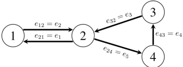
2.4 New indices𝑘 for the edges in a graph. . . 31
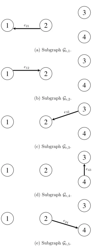
2.5 Example of subgraphs on edges. . . 32
3.1 Regular directed network with four agents. . . 59
3.2 State trajectories and error for 𝜏 = 1s. . . 61
3.3 State trajectories and error for 𝜏 = 5s. . . 62
3.4 State trajectories and error for 𝜏 = 10s. . . 63
3.5 State trajectories and error for 𝜏 = 2s. . . 65
3.6 State trajectories and error for 𝜏 = 4s. . . 66
3.7 State trajectories and error for 𝜏 = 7s. . . 67
3.8 State trajectories and error for 𝜏 = 8s. . . 68
3.9 Directed network with four agents. . . 73
3.10 State trajectories and error for 𝜏 = 0.07s. . . 76
3.11 State trajectories and error for 𝜏 = 0.35s. . . 77
3.12 State trajectories and error for 𝜏 = 0.44s. . . 78
4.1 Directed network with four agents. . . 88
4.2 Time-varying delay𝜏𝑘(𝑡)with random amplitude. . . 89
4.3 State trajectories and error with communication delay given by 𝜏 = 0.30 and 𝜇𝑚= 0.20. . . 91
5.1 Multi-agent system subject to input delays 𝜏𝑖(𝑡), composed of three agents with switching topologies 𝒢1 and 𝒢2. . . 105
5.2 Multi-agent system subject to communication delays 𝜏(𝑡), composed of three agents with switching topologies 𝒢1 and 𝒢2. . . 105
5.3 Simulation with time-varying delay and switching topologies with 𝜏 = 0.15 and 𝜇𝑚 = 0.10. . . 107
6.1 Coupling strengths𝑎𝑖𝑗 to be designed. . . 110
6.2 Directed graph of the network topology with indices 𝑖, 𝑗 in (a), and 𝑘 in (b) after the application of Algorithm 2.1. . . 117
6.3 The state trajectories for the multi-agent system in Fig. 6.2, with unitary coupling strengths, subject to multiple time-varying delays𝜏𝑖(𝑡)∈[0.55, 0.65], and initial states 𝑝(0) = [8 5 2 0 −2 −5 −8]𝑇. . . 118
6.4 The state trajectories for the multi-agent system in Fig. 6.2 subject to multiple time-varying delays 𝜏𝑖(𝑡) ∈ [0.55, 0.65], with initial states 𝑝(0) = [8 5 2 0 − 2 −5 −8]𝑇 and designed coupling strengths by Theorem 6.1 for: (a) very small 𝛿 >0 and 𝑔 = 1; (b) 𝛿 = 0.19and 𝑔 = 0.8. . . 119
6.5 Feasibility of Theorem 6.1 for various pairs (𝑔, 𝛿), with 𝑔 ranging from 0 to4 with a step size of 0.1 and 𝛿 ranging from 0.1 to 0.2 with a step size of 0.01. A feasible pair is represented by cross, and an unfeasible one by dot. . . 119
6.6 Simulation for fully connected network with coupling strengths designed by Qiao and Sipahi (2013) and constant time-delay 𝜏 = 0.027. . . 120
6.7 Simulation for fully connected network with coupling strengths designed by Theorem 6.1 and constant time-delay 𝜏 = 0.027. . . 121
Theorem 6.1 with non-differentiable time-varying delay in the range [1,2.2]. . . 122
6.10 Graphs 𝒢(1) and 𝒢(2) representing the two possible topologies of the multi-agent system. . . 123
6.11 State trajectories of the multi-agent system in the numerical example without any design of the coupling strengths. The initial states are𝑥(0) = [4 2 1 −2]𝑇.124 6.12 Switches of the topology for one simulation, where 𝑙 = 1,2 are the Markov chain states. . . 124
6.13 State trajectories of the multi-agent system in the numerical example with the designed coupling strengths. . . 125
7.1 Each agent has a desired relation with the center of formation. The information exchanged is each agent’s opinion on this center. . . 136
7.2 Network topology. . . 138
7.3 Simulation for five agents in a circular formation. . . 139
7.4 Time-evolution for each part of the output. . . 140
7.5 Simulation for 300 agents in a circular formation. . . 141
7.6 Network topology. . . 144
7.7 Experiment on formation with KUKA YouBots. . . 145
7.8 Measure and simulation of each part of the output of each agent in the exper-iment on formation with two KUKA YouBots. . . 146
3.1 Elements of Ψ . . . 63
3.2 Consensusability switches analysis . . . 64
3.3 Elements of Ψ . . . 75
3.4 Consensability switches . . . 75
4.1 Maximum allowed constant input delay 𝜏𝑖(𝑡) = 𝜏 obtained for multiagent system in Figure 4.1. . . 89
4.2 Maximum allowed constant communication delay𝜏(𝑡) = 𝜏 obtained for multi-agent system in Figure 4.1. . . 89
4.3 Largest 𝛿 obtained for input delays with given pair (𝜏, 𝜇) . . . 90
4.4 Largest 𝛿 obtained for communication delays with given pair (𝜏, 𝜇) . . . 90
5.1 Largest 𝜇𝑚 obtained for given 𝜏 . . . 106
5.2 Largest 𝛿¯obtained for given (𝜏, 𝜇𝑚,𝜋¯) . . . 106
R Set of Real Numbers.
N Set of Natural Numbers.
Z Set of Integer Numbers.
H Set of Quaternions.
E Expectancy.
ℋ Set of Dual Quaternions.
𝑀𝑇 Transpose of a matrix𝑀.
˙
𝑥(𝑡) First time-derivative of 𝑥(𝑡).
¨
𝑥(𝑡) Second time-derivative of 𝑥(𝑡).
𝒢 Simple Directed Graph.
I𝑛 Identity Matrix of size 𝑛.
1𝑛 Column-vector of ones with size 𝑛.
0𝑛 Column-vector of zeros with size 𝑛.
0 Zero matrix with appropriate dimension.
⊗ Kronecker Product
𝑀 >0 Denotes a Positive Definite Matrix 𝑀.
𝑀 <0 Denotes a Negative Definite Matrix 𝑀.
𝑀† Moore-Penrose pseudoinverse of 𝑀.
min(𝑥, 𝑦, ..., 𝑧) Returns the minimum value of the arguments.
sign(𝑥) Returns sign of the argument𝑥.
∅ Empty set.
det(𝑀) Determinant of a matrix 𝑀.
x Denotes a quaternion.
x Denotes a dual quaternion.
| · | Module operator.
|| · || Norm operator.
* In a matrix represents a symmetric, transpose, element.
𝜆𝑖{·} The 𝑖-th eigenvalue of a matrix.
𝜆max{·} The maximum eigenvalue of a matrix.
𝜆min{·} The minimum eigenvalue of a matrix.
diag{𝑑1, . . . , 𝑑𝑛} Diagonal matrix with elements 𝑑1, . . . , 𝑑𝑛 in the main diagonal.
sup{·} Supremum element in a set.
ℱ Reference frame.
𝐺⋉𝐻 Denotes the semidirect product of a group𝐺 by a group 𝐻.
LMI Linear Matrix Inequality.
BMI Bilinear Matrix Inequality.
MJLS Markov Jump Linear System.
LKF Lyapunov-Krasovskii Functional.
1 Introduction 1
1.1 History . . . 2
1.1.1 Consensus in Robotics . . . 3
1.2 Consensus Protocol . . . 4
1.3 Time-delay in Consensus Protocol . . . 6
1.4 First-order Dynamics . . . 9
1.4.1 Consensus-based Formation . . . 10
1.5 Second-order Dynamics . . . 14
1.5.1 Consensus-based Flocking . . . 16
1.6 High-order Dynamics . . . 17
1.6.1 Consensus-based Platooning . . . 20
1.7 Overview of this Thesis and Contributions . . . 22
2 Background for Analyzing Consensus as Stability 26 2.1 Algebraic Graph Theory . . . 26
2.1.1 Ordered Index for the Edges . . . 29
2.1.2 Alternative Representation of the Laplacian Matrix . . . 31
2.2 Consensus Problem Formulation . . . 33
2.2.1 Tree-type Transformation . . . 34
2.2.2 Consensus Problem with Communication Delay . . . 35
2.2.3 Consensus Problem with Input Delay . . . 40
2.2.4 Consensus free of Time-Delays . . . 43
2.3 Additional Lemmas . . . 45
3 Consensus with Constant Time-Delays: Exact Conditions 47 3.1 Dynamics free of Delay . . . 48
3.2 Dynamics with Communication Delay . . . 50
3.2.1 Analysis . . . 50
3.2.2 Consensus on Time-Delay Intervals . . . 52
3.2.3 Numerical Examples . . . 59
3.3 Dynamics with Input Delay . . . 65
3.3.2 Consensus on Time-Delay Intervals . . . 69
3.3.3 Numerical Examples . . . 73
4 Consensus with Time-Varying Delays: Sufficient Conditions 79 4.1 Consensus analysis . . . 80
4.2 Numerical Examples . . . 87
4.2.1 Constant Delays . . . 88
4.2.2 Time-varying Delays . . . 89
5 Consensus Analysis with Switching Topologies 92 5.1 Problem Formulation with Switching Topologies . . . 93
5.2 Consensus analysis . . . 97
5.3 Numerical Example . . . 103
6 Design of the Coupling Strengths for Agents with First-Order Inte-grator Dynamics 109 6.1 Fixed Topology . . . 110
6.2 Switching Topology . . . 113
6.3 Numerical Examples for fixed topology . . . 116
6.3.1 Fully connected network with constant time-delay . . . 120
6.3.2 Fully connected network with non-differentiable time-varying delay 121 6.4 Numerical Example for Switching Topologies . . . 122
7 Dual Quaternion Pose-Consensus and Robotics 126 7.1 Dual quaternions . . . 127
7.2 Dual Quaternion Consensus . . . 131
7.3 Pose Consensus . . . 133
7.4 Consensus-Based Formation . . . 135
7.5 Examples . . . 138
7.6 Whole Body Kinematics Model . . . 139
7.6.1 Mobile Manipulators Formation Control . . . 143
7.6.2 Experiment with two real KUKA youBots and a fixed reference . . 143
7.6.3 Application of the main result in cooperative manipulation . . . 145
Conclusion 148 List of Publications . . . 152
Introduction
There is a growing interest in systems composed of multiple agents that work coopera-tively by sharing information in a networked manner. This growth is mainly given due to the recent advances in communication systems, with the ease to enable digitally controlled devices to work connected in a network. In addition to the reduction in size and cost of electromechanical devices and the boost in computational power, networked systems have become an increasingly recurrent scenario. This kind of systems is referred to as multi-agent system, i.e. a system composed of several distributed parts, sharing information and working cooperatively in order to accomplish a common objective (Tanenbaum and Van Steen, 2007). In fact, one of the most important attributes of an intelligent system is the ability to communicate. Communicating and sharing information allows an agent to distribute/cooperate in tasks. The distribution of tasks makes the multiagent system robust to failures and endows intelligent group behavior. In addition, it mainly allows the execution of tasks that a single agent would not be able to accomplish, e.g. the trans-portation of heavy duty loads. Some cutting-edge applications of multiagent systems can be highlighted in topics like Internet of Things (Greengard, 2015), Cloud Computing (Ru-parelia, 2016), and Cloud Robotics, referred to as one of the 10 breakthrough technologies for the year 2016 (Schaffer, 2016).
One of the ongoing topics covered by the theory of multiagent systems is called con-sensus. The meaning of consensus problem is to make all the agents in a multiagent system achieve an agreement on a variable of interest, assuming that each agent is able to share and/or acquire information within a subset of other agents, called neighbors. Applications of consensus are found in many practical fields, such as traffic jams in com-munication networks (Li et al., 2011b), formation of autonomous mobile agents (Ren, 2007), page ranking (Ishii and Tempo, 2014), robotics (Hatanaka et al., 2015), etc. Many other results are summarized by Cao et al. (2013). Next section covers an overview and part of the history of this topic.
Consensus problem has its origins in statistics, in the decades of 1960 and 1970. At that time, the main concern was with the problem of social learning process, and some methods were presented to describe how a group of individuals reach an agreement about a common goal. This problem was discussed by many authors, among those it can be referred the works of Eisenberg and Gale (1959), Stone (1961), Norvig (1967), and Winkler (1968). The work of DeGroot (1974) can be highlighted, it once described a group of individuals acting together as a team, in which each individual had its own subjective probability distribution regarding the opinion about some given parameter. The author described a model on how the team achieves a common subjective probability distribution through the exchange of information and the combination of the individuals’ beliefs by weighting and averaging the opinions, deprived of taking any new information from the environment.
Later on, with the advent of coordinated multiagent systems, one of the major prob-lems was the one of establishing distributed control laws based on the information ex-changed between the agents, such that an agreement could be achieved on a common value of a given variable of interest. Seminal results emerged in physics (Vicsek et al., 1995) and distributed algorithms (Lynch, 1996), borrowing the main ideas of consensus originated in the field of statistics regarding the exchange of information between the agents.
The work of Vicsek et al. (1995) described the self-ordered motion of a system com-posed of multiple particles. At each time step, each particle assumed the average direction of neighboring particles in a given distance radius, introducing in multiagent systems the concept of neighborhood and the interaction with neighbors only. This inspiration came from parallel advances in the field of biology and computer graphics, in the biological de-scription of the function of fish schools (Partridge, 1982), and from the behavioral models of flocks, herds and schools for computer graphic simulations in the work by Reynolds (1987).
At the end of the 90’s, the problem of flight formation arose as one of the enabling technologies for the 21st
century. The purpose was to extend the control of a single spacecraft to the control of a group of it, flying in a particular designated arrangement. Some authors like the ones by Wang et al. (1999), Mesbahi and Hadaegh (1999), and Mesbahi and Hadaegh (2001) considered the leader-following model, and the latter can be emphasized by the usage of the graph interpretation of the problem and also the derivation of control laws based on Linear Matrix Inequalities (LMIs).
of robotics. Research was focused on the extension of motion planning algorithms to the control of multiple robots in a distributed manner, as pointed by Wang and Beni (1988) and Sugihara and Suzuki (1990). The purpose was to enable a group of robots to cooperate in order to accomplish a global task under the government of a protocol (a distributed algorithm), executed individually by each robot. These simple protocols borrowed ideas from Cellular Automata (Neumann and Burks, 1966), in which global complex tasks can be accomplished with the cooperation between many agents with the execution of simple individual rules. Some of the results refer to the formation of circular patterns (Tanaka, 1992), and, further, to more general geometric patterns (Suzuki and Yamashita, 1999).
Within all the theoretical advances, it was noted that the control architecture of a multiagent system is strongly affected by the corresponding sensing and communication topology (Mesbahi and Hadaegh, 2001; Mesbahi, 2002). At that point, Fax and Mur-ray (2002) and Jadbabaie et al. (2003) applied the algebraic theory of graphs to write the relationship between neighboring agents as presented in the work of Vicsek et al. (1995). Henceforth, the network topology could be described algebraically, inheriting terms from graph theory like: directed, when the information flow can be unidirectional; or undirected, when the flow is bidirectional. This algebraic approach assisted on better understanding the impacts of the topology and model the multiagent dynamics, and many other results emerged, such as the ones by Olfati-Saber and Murray (2003), Olfati-Saber and Murray (2004), Ren and Beard (2005), etc. The present work makes use of this algebraic approach.
1.1.1
Consensus in Robotics
Some recent works have considered the problem of consensus in robotic networks composed of multiple mobile manipulators, in which the objective might be to achieve a common configuration on the joints in order to execute some tasks, like grasping or carrying an object. The work by Cheng et al. (2008) considered the uncertainties in the model of the manipulators and showed an adaptive consensus protocol to reach consensus on the joints. Hou et al. (2009) considered also the presence of external disturbances. In the work of Ge and Dongya (2014) the problem of consensus is treated using robust control techniques. Most of these works have dealt with Euler-Lagrange models, and some have also considered a model description that uses quaternions to represent orientation (Aldana et al., 2015). Additionally, the application of dual quaternions is of great interest since complex systems can be easily modeled with dual quaternions using a whole-body approach (Adorno, 2011).
NEIGHBORING AGENTS:Ni
Consensus Protocol Agenti
Agentj
.. .
Agentk
𝑥𝑖(𝑡)
𝑥𝑗(𝑡)
𝑥𝑘(𝑡)
..
.
Control input
u𝑖(𝑡)
Figure 1.1: Block diagram for the consensus protocol.
may benefit from solutions of formation control, such as cooperative load transportation to move flexible payloads (Bai and Wen, 2010). Besides, rigid formation problems have also been considered by Mou et al. (2014) and Sun et al. (2015).
Next section presents and describes the application of consensus protocol with an introductory example.
1.2
Consensus Protocol
In the literature, the distributed control law devised to drive the agent states to consensus is commonly denominated as consensus protocol. The protocol provides the agent’s control input and is usually based on the difference between the agent’s own state and the states of its neighbors. Figure 1.1 illustrates the application of the consensus protocol by an arbitrary agent𝑖 in a multiagent system. The neighboring agents of 𝑖 are represented by the set 𝑁𝑖, such that 𝑗, . . . , 𝑘 ∈ 𝑁𝑖. The agent’s local state is represented by 𝑥𝑖(𝑡) ∈ R and the state of a neighboring agent 𝑗 or 𝑘 is represented by 𝑥𝑗(𝑡) ∈ R or 𝑥𝑘(𝑡) ∈ R, respectively. The protocol is any function taking into account the agent’s local state and all the states of its neighbors 𝑓𝑖 = (𝑥𝑖, 𝑥𝑗, . . . , 𝑥𝑘), 𝑗, . . . , 𝑘 ∈ 𝑁𝑖, and is executed locally by each agent. The protocol returns the control inputu𝑖(𝑡)∈Rfor an agent𝑖. The most prevailing consensus protocol in the literature is the linear consensus protocol introduced by Olfati-Saber and Murray (2003), given by
u𝑖(𝑡) =−
∑︁
𝑗∈𝑁𝑖
𝑎𝑖𝑗(𝑥𝑖(𝑡)−𝑥𝑗(𝑡)), (1.1)
where𝑎𝑖𝑗 is the gain related to the information from agent 𝑗 to agent 𝑖, for all 𝑗 ∈𝑁𝑖.
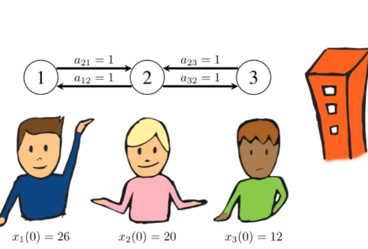
want to build, as shown in Figure 1.2. The blue individual (agent1) wants a building with a height of 26m, the pink individual (agent2) wants a height of 20m, and the green one (agent 3) suggests 12m. Therefore, the initial conditions of this problem are 𝑥1(0) = 26,
𝑥2(0) = 20, and𝑥3(0) = 12. The next step is to define the network topology and the gains
𝑎𝑖𝑗 related to the communication links. If the individuals can only talk to the immediate neighbors the information flow can be defined as in Figure 1.2, where agent 2 can listen to both agents 1 and 2, with 𝑎21 = 𝑎23 = 1, and the others can only listen to agent 2,
𝑎12 = 1 and 𝑎32 = 1. With this information, protocol (1.1) can be applied, and one can consider that the assumption that each individual opinion varies continuously according to
˙
𝑥𝑖(𝑡) =u𝑖(𝑡). (1.2)
1
2
3
a21= 1
a12= 1
a23= 1
a32= 1
x1(0) = 26 x2(0) = 20 x3(0) = 12
Figure 1.2: Individuals consensus problem.
With these parameters defined, a simulation is carried out to show the evolution of the individuals’ opinions as consensus is reached, presented in Figure 1.3. The representation of the agents’ states along time presented in Figure 1.3 will be widely used in this text to show whether consensus is achieved or not. From this figure the final value and the time spent to achieve consensus can be assessed. For this example, the individuals reach a consensus that the height of the building to be constructed is the consensus value as time goes to infinitylim𝑡→∞𝑥𝑖(𝑡)≈19.3m.
xi
(
t
)
t
0 1 2 3 4 5 6 7 8
14 16 18 20 22 24
NEIGHBORING
AGENTS:Ni COMMUNICATION DELAYS: τij(t),. . . ,τik(t), respectively
Consensus Protocol Agenti
Agentj
Channel Induced Delay ..
. Agentk
Channel Induced Delay
𝑥𝑖(𝑡)
𝑥𝑗(𝑡) 𝑥𝑗(𝑡−𝜏𝑖𝑗(𝑡))
.. .
𝑥𝑘(𝑡) 𝑥𝑘(𝑡−𝜏𝑖𝑘(𝑡))
Control input
u𝑖(𝑡)
.. .
Figure 1.4: Block diagram for the consensus protocol with communication delays.
More recently, the topic of consensus has been considered to deal with a variety of scenarios. Major concerns have been in the consideration of real issues arising from the application of communication networks, specifically time-delays and switching topologies. An overview with the implications of delays is presented in the next section.
1.3
Time-delay in Consensus Protocol
In practice, time-delays are always present in the agents’ interactions. This is mainly given due to computational and physical limitations in information processing, transmission channels, time-response of actuators, etc. The presence of delays has a great impact on consensus problems as it can make the system oscillate or diverge about the variable of interest (Lin et al., 2009). Based on this fact, many works have dealt with consensus problems subject to different forms of time-delays.
The class of delays given by the time spent by an agent𝑖 to acquire information from an agent𝑗 —or the time spent to carry information from the𝑗-th agent to the𝑖-th agent— which can arise naturally due to physical characteristics of communication channels or sensing, is called communication delay. This delay can be represented by 𝜏𝑖𝑗(𝑡), and essentially indicates how old is the information that agent 𝑖 has from agent 𝑗, at the instant of time 𝑡 when agent 𝑖 is locally running the consensus protocol. The occurrence of communication delays is illustrated in Figure 1.4, where the consensus protocol has access to the local agent’s state 𝑥𝑖(𝑡) instantly, but the states of the neighboring agents
𝑗 to 𝑘 are delayed by 𝜏𝑖𝑗(𝑡) and 𝜏𝑖𝑘(𝑡), i.e 𝑥𝑗(𝑡−𝜏𝑖𝑗(𝑡)) and 𝑥𝑘(𝑡−𝜏𝑖𝑘(𝑡)), respectively. Additionally, communication delays can exist and be different for each neighboring agent, as the agents 𝑗 and 𝑘 can be subject to different delays 𝜏𝑖𝑗(𝑡)̸=𝜏𝑖𝑘(𝑡).
with a single integrator dynamics as in (1.2) is able to achieve consensus regardless of communication delays, as long as the information from one of the agents can reach all the other agents. This network constraint will be presented later as the existence of a directed spanning tree in the graph that describes the communication topology. Consensus is achieved by applying the linear consensus protocol introduced by Olfati-Saber and Murray (2003), by writing (1.1) with the communication delays𝜏𝑖𝑗(𝑡)as
u𝑖(𝑡) =−
∑︁
𝑗∈𝑁𝑖
𝑎𝑖𝑗(𝑥𝑖(𝑡)−𝑥𝑗(𝑡−𝜏𝑖𝑗(𝑡))). (1.3)
To illustrate the effects of communication delays in agents whose dynamics are de-scribed by (1.2) subject to protocol (1.3), the same parameters and initial conditions for the example in the previous section are considered in a simulation, with the addition of a very large communication delay𝜏𝑖𝑗 =𝜏 = 10s, ∀𝑗 ∈𝑁𝑖. The state trajectories are shown in Figure 1.5, showing the tendency of the agents to achieve consensus. As expected from Moreau (2004), the communication time-delay did not prevent the agents to achieve con-sensus, but did affect convergence time when compared to Figure 1.3. Some results will be presented in the next chapters showing that communication delays can indeed prevent consensus achievement for more complex dynamics.
xi
(
t
)
t
0 50 100 150 200 250 300 350 400 14
16 18 20 22 24
Figure 1.5: Consensus with very large communication delay.
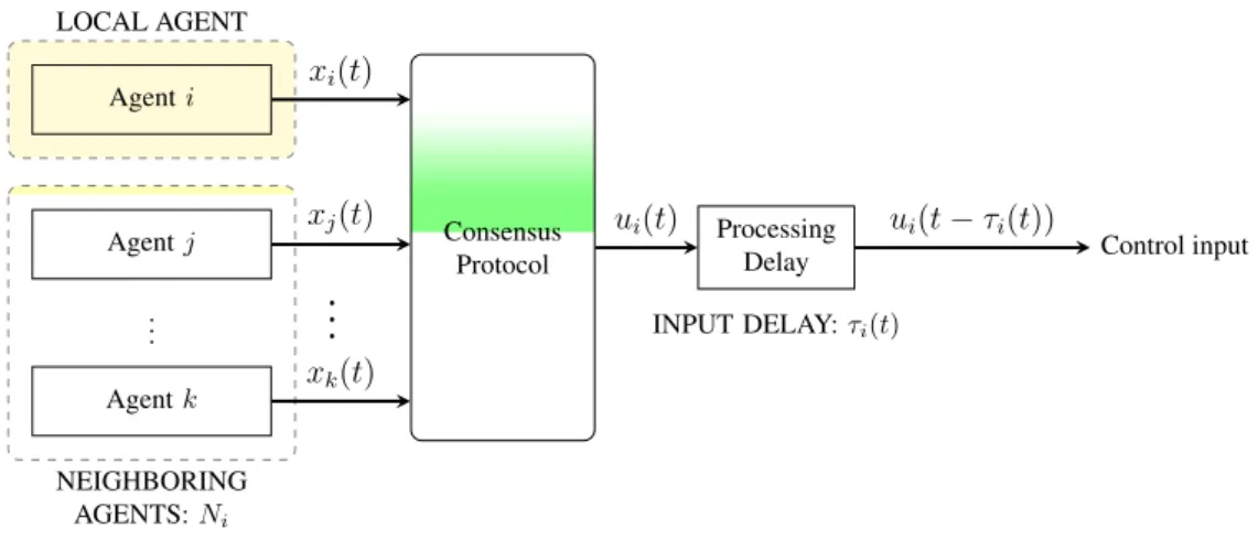
Another common type of time-delay is the one in the control inputs, given by the time-response of actuators and information processing. This is called input delay and is represented by𝜏𝑖(𝑡). It is locally present in agent𝑖and affects the action of the controller, representing how much time it takes for the control action to be executed. The occurrence of input delays is illustrated in Figure 1.6, where the protocol has access to all the states instantaneously, but its action is delayed by 𝜏𝑖(𝑡). This effect acts at instant of time 𝑡, for agent 𝑖, as if all the states where delayed by 𝜏𝑖(𝑡), with 𝑥𝑖(𝑡−𝜏𝑖(𝑡)) and 𝑥𝑗(𝑡−𝜏𝑖(𝑡)). The input delays can also exist and be different for each agent, such that each𝑖-th agent is subject to a different delay𝜏𝑖(𝑡).
NEIGHBORING AGENTS:Ni
Consensus Protocol Agenti
Agentj Processing
Delay ..
. Agentk
𝑥𝑖(𝑡)
𝑥𝑗(𝑡)
𝑥𝑘(𝑡)
.. .
u𝑖(𝑡) u𝑖(𝑡−𝜏𝑖(𝑡))
Control input
INPUT DELAY:τi(t)
Figure 1.6: Block diagram for the consensus protocol with input delays.
Figure 1.6 is given by
u𝑖(𝑡) = −
∑︁
𝑗∈𝑁𝑖
𝑎𝑖𝑗(𝑥𝑖(𝑡−𝜏𝑖(𝑡))−𝑥𝑗(𝑡−𝜏𝑖(𝑡))). (1.4)
The analysis of multiagent systems with delayed consensus protocols as (1.3) and (1.4) are held in order to find the delay margins that allow consensus. Accordingly, consensus with time-delays has been treated under many perspectives and many results can be found in the works by Olfati-Saber and Murray (2003), Olfati-Saber and Murray (2004), Moreau (2005), Ren and Beard (2005), Lin et al. (2008), Bliman and Ferrari-Trecate (2008), and Sakurama and Nakano (2015), for example.
For the same previous example, considering all the agents with the same delay𝜏𝑖 =𝜏, the maximum input delay 𝜏max that would allow consensus according to Olfati-Saber and Murray (2004) is𝜏max = 0.5236. Figure 1.7 shows a simulation with an input delay
𝜏 = 0.55, greater than the margin𝜏max, to verify and show that consensus is not achieved.
xi
(
t
)
t
0 5 10 15 25 30
14 16 18 20
20 22
24
Figure 1.7: Input delay higher than upper margin preventing consensus.
Considering the consensus protocol with input delays, Lin et al. (2008) obtained a sufficient condition for directed networks including also external disturbances and model uncertainties. Bliman and Ferrari-Trecate (2008) extended the work of Olfati-Saber and Murray (2003) for time-delays to the cases with time-varying topologies, showing ana-lytical necessary and/or sufficient conditions to reach consensus. Kecai et al. (2011) and Zhang et al. (2011) studied differentiable and nonuniform time-varying delays, where the delays can be time-varying satisfying0≤𝜏𝑖𝑗(𝑡)≤𝜏𝑖𝑗maxand also be different for each com-munication link. Some authors, like Sun and Wang (2009) and Xi et al. (2013), considered the possibility of nonuniform and also non-differentiable time-varying delays, such that the variation of the delay is unknown. These results were limited to agents with single integrator dynamics
Results considering time delay and second-order integrator dynamics can be found in the work of Pan et al. (2014), which shows necessary conditions for constant and uniform time delays for undirected networks. For directed networks, Yu et al. (2010) shows some sufficient results.
To contextualize and highlight the different classes of multiagent systems that will be addressed in the text, next section covers some examples of multiagent systems with first-order dynamical systems with an example in formation control, second-first-order dynamics with an example in flocking, and high-order dynamics applied to the control of vehicles in a platoon.
1.4
First-order Dynamics
First-order dynamics agents are referred to agents with a single integrator, with the consensus protocol acting directly on the agent’s “velocity”. The dynamics of this kind of agent is given by (1.2) and repeated here for convenience:
˙
𝑥𝑖(𝑡) =u𝑖(𝑡). (1.5)
X y1
x1 y2
x2 y3
x3 y4
x4
Agent1
Agent2
Agent3
Agent4
Figure 1.8: Agents placement in the two-dimensional plane.
Y
X
(x∗
1, y1∗) (x∗2, y∗2)
(x∗
3, y3∗) (x∗4, y∗4)
Figure 1.9: Desired agents’ formation.
1.4.1
Consensus-based Formation
One of the most prevailing applications on multi-vehicle systems is the formation problem. The purpose is that the agents collectively maintain a prescribed geometry, considering decentralized control and prior knowledge of the desired formation shape. The desired shape can be either set by a centralized reference or programmed on each agent. Fi-nally, the system is able to achieve formation anywhere in the space, depending on the negotiation among the team members.
To illustrate this problem in a consensus-based approach, consider holonomic vehicles able to move in a two-dimensional space. The state of each agent is described by the coordinates (𝑥𝑖, 𝑦𝑖), ∀𝑖, with respect to the𝑋 and 𝑌 axis, according to Figure 1.8.
Next, the desired agents’ positions are drawn in an arbitrary position in the space respecting the desired relative positions. Figure 1.9 shows the desired agents’ formation represented by the blue dots, and coordinates (𝑥*
Y
X
δ1 δ2
δ3
δ4
Figure 1.10: Distance 𝛿𝑖 to the formation position.
Y
X
δ1 δ2
δ3 δ4
Figure 1.11: Consensus on the distance – formation.
The consensus-based approach to keep formation is that all the agents must achieve consensus on the displacement between the reference of the desired formation and the actual position. The displacement vector𝛿𝑖 ∈R2,∀𝑖, in Figure 1.10, represents this error, with
𝛿𝑖 =
[︃
𝑥𝑖−𝑥*𝑖
𝑦𝑖−𝑦𝑖*
]︃
. (1.6)
Following the results presented by Ren (2007), formation is achieved when the agents achieve consensus on 𝛿𝑖. Figure 1.11 shows the case when the agents have achieved the squared desired formation in a different part of the two-dimensional plane, showing equal displacement vectors𝛿𝑖.
Thus, the consensus protocol to achieve formation is u𝑖 ∈R2,
u𝑖(𝑡) = −
∑︁
𝑗∈𝑁𝑖
𝑎𝑖𝑗(𝛿𝑖(𝑡)−𝛿𝑗(𝑡)), (1.7)
3
1
4
2
a12= 1a2
4
=
1
a3
1
=
1
Figure 1.12: Network topology represented as a graph.
given by 𝛿𝑥,𝑖=𝑥𝑖(𝑡)−𝑥*𝑖 and 𝛿𝑦,𝑖=𝑦𝑖(𝑡)−𝑦*𝑖, yielding
u𝑥,𝑖(𝑡) =−
∑︁
𝑗∈𝑁𝑖
𝑎𝑖𝑗
(︀
(𝑥𝑖(𝑡)−𝑥*𝑖)
⏟ ⏞
𝛿𝑥,𝑖
−(𝑥𝑗(𝑡)−𝑥*𝑗)
⏟ ⏞
𝛿𝑥,𝑗
)︀
, (1.8)
u𝑦,𝑖(𝑡) = −
∑︁
𝑗∈𝑁𝑖
𝑎𝑖𝑗
(︀
(𝑦𝑖(𝑡)−𝑦𝑖*)
⏟ ⏞
𝛿𝑦,𝑖
−(𝑦𝑗(𝑡)−𝑦𝑗*)
⏟ ⏞
𝛿𝑦,𝑗
)︀
, (1.9)
such that the agents are controlled by inputs which are velocities given by
𝑣𝑥(𝑡) =u𝑥,𝑖(𝑡), (1.10)
𝑣𝑦(𝑡) =u𝑦,𝑖(𝑡), (1.11)
where 𝑣𝑥(𝑡) and 𝑣𝑦(𝑡) are the velocities on 𝑋 and 𝑌 axis, respectively, and are indepen-dently set.
A simulation is carried out to illustrate the formation problem. Considering the state of each agent given by
𝑞𝑖(𝑡) =
[︃ 𝛿𝑥,𝑖(𝑡)
𝛿𝑦,𝑖(𝑡)
]︃
, (1.12)
with initial conditions considered 𝑞1(0) = [−1 0.5]𝑇, 𝑞2(0) = [2 0]𝑇, 𝑞3(0) = [−0.5 1]𝑇, and𝑞4(0) = [−1 1]𝑇, and given that the desired formation is a square given by(𝑥*1, 𝑦*1) =
(0,0), (𝑥*
2, 𝑦2*) = (1,0), (𝑥*3, 𝑦3*) = (0,1), and (𝑥*4, 𝑦4*) = (1,1). The communication net-work is such that agent 1 receives information from agent 2 (𝑎12 = 1), agent 2 receives information from agent 4 (𝑎24 = 1), agent 4 receives information from agent 3 (𝑎43= 1), and agent3receives information from agent1(𝑎31= 1). The network topology describing this information flow can be graphically represented by the graph in Figure 1.12.
The state trajectories are shown in Figure 1.13. Figure 1.13a shows the convergence for the state variable 𝛿𝑥,𝑖(𝑡) and Figure 1.13b for 𝛿𝑦,𝑖(𝑡), both converging approximately at 𝑡 = 5𝑠. Additionally, the trajectories of the agents in the two-dimensional plane 𝑋𝑌
are illustrated in Figure 1.14. The initial state 𝑞𝑖(0) is represented at the initial position
δx,i
(
t
)
t
−0.5 0
0 0.5
1
1 1.5
2 3 4 5 6
(a) State trajectories forδ𝑥,𝑖(t)for all agents.
δy
,i
(
t
)
t
0 1 2 3 4 5 6
0.2 0.4 0.6 0.8
(b) State trajectories forδ𝑦,𝑖(t) for all agents.
Figure 1.13: State trajectories for first-order agents formation.
Y
X
−1
−1
−0.5
−0.5
0
0
0.5
0.5
1
1
1.5
1.5
2
2
2.5
2.5 3
q1(0)
q2(0)
q3(0) q4(0)
(x∗
1, y1∗) (x∗2, y∗2)
(x∗
3, y3∗) (x∗4, y∗4)
q1(5)
q2(5)
q3(5)
q4(5)
Figure 1.14: Simulated state trajectories for single-order agents achieving formation.
approximately stationary state𝑞𝑖(5) at time𝑡 = 5𝑠, with circles representing the position
(𝑥𝑖, 𝑦𝑖)at time-steps of 0.02𝑠. The dashed lines represent the final displacements between the agents and the reference positions(𝑥*
1, 𝑦*1) = (0,0), (𝑥*2, 𝑦2*) = (1,0), (𝑥*3, 𝑦*3) = (0,1), and (𝑥*
Some agents are assumed to obey a second-order model to describe its dynamics. This model is suitable for mechanical systems controlled through acceleration (force or torque). For example, thrust-propelled vehicles (Wang, 2016), or more generally agents that can be feedback linearized as double integrators, as it will be presented next.
A second-order integrator agent is given by the state variables 𝑥𝑖 ∈ R and 𝑥˙𝑖 ∈ R, which can represent, for example, position and velocity, respectively. The dynamics is given such that
¨
𝑥𝑖(𝑡) =u𝑖(𝑡), (1.13)
where the control input represents an “acceleration”.
An example from Ren and Atkins (2007) is presented to illustrate the description of a non-holonomic mobile robot with second-order dynamics. The equations of motion are given by
˙
𝑥𝑖 =𝑣𝑖cos(𝜃𝑖), (1.14)
˙
𝑦𝑖 =𝑣𝑖sin(𝜃𝑖), (1.15)
˙
𝜃𝑖 =𝜔𝑖, (1.16)
𝑚𝑖𝑣˙𝑖 =𝐹𝑖, (1.17)
𝐽𝑖𝜔˙𝑖 =𝑇𝑖, (1.18)
where (𝑥𝑖, 𝑦𝑖) is the position of the robot center, 𝜃𝑖 is the orientation, 𝑣𝑖 is the linear velocity, 𝜔𝑖 is the angular velocity, 𝑚𝑖 is the mass, 𝐽𝑖 is the moment of inertia, 𝐹𝑖 is the force, and𝑇𝑖 is the torque applied to the robot. An illustration for this agent is given in Figure 1.15a.
Next, to avoid the issue introduced by the non-holonomic constraints, a point(𝑥ℎ𝑖, 𝑦ℎ𝑖) at a distance 𝑑𝑖 off the wheel axis as in Figure 1.15b is considered in order to define the outputs:
[︃ 𝑥ℎ𝑖
𝑦ℎ𝑖
]︃
=
[︃ 𝑥𝑖
𝑦𝑖
]︃
+𝑑𝑖
[︃
cos(𝜃𝑖)
sin(𝜃𝑖)
]︃
. (1.19)
Let
[︃ 𝐹𝑖
𝑇𝑖
]︃
=
[︃
1
𝑚𝑖cos(𝜃𝑖) − 𝑑𝑖
𝐽𝑖 sin(𝜃𝑖) 1
𝑚𝑖sin(𝜃𝑖) 𝑑𝑖
𝐽𝑖 cos(𝜃𝑖)
]︃−1[︃
u𝑥𝑖+𝑣𝑖𝜔𝑖sin(𝜃𝑖) +𝑑𝑖𝜔2𝑖 cos(𝜃𝑖)
u𝑦𝑖−𝑣𝑖𝜔𝑖cos(𝜃𝑖) +𝑑𝑖𝜔2𝑖 sin(𝜃𝑖)
]︃
, (1.20)
where u𝑥𝑖 and u𝑦𝑖 are the acceleration inputs, related to the velocities 𝑣𝑥𝑖 and 𝑣𝑦𝑖, of
Y
X yi
xi
Fi
Ti
θi
(a) Mobile robot controlled by force and torque.
Y
X
•
yi
xi yhi
xhi θi di
vxi vyi
(b) Mobile robot with a reference point off wheel axis for linearization.
Figure 1.15: Linearization of second-order agent.
obtained:
˙
𝑥ℎ𝑖 =𝑣𝑥𝑖, (1.21)
˙
𝑣𝑥𝑖 =u𝑥𝑖, (1.22)
˙
𝑦ℎ𝑖 =𝑣𝑦𝑖, (1.23)
˙
𝑣𝑦𝑖 =u𝑦𝑖. (1.24)
Finally, the pairs of equations (1.21)–(1.22) and (1.23)–(1.24) are in the form of (1.13), and thus the system can be analyzed as second-order integrator agents and consensus-based results can be applied.
u𝑖(𝑡) =−
∑︁
𝑗∈𝑁𝑖
𝑎𝑖𝑗(𝛼2(𝑥𝑖(𝑡)−𝑥𝑗(𝑡)) +𝛼1( ˙𝑥𝑖(𝑡)−𝑥˙𝑗(𝑡))), (1.25)
where𝛼1 and 𝛼2 are the gains in the consensus protocol related to each state variable.
1.5.1
Consensus-based Flocking
A framework similar to the one applied in formation control problem can be used in order to describe flocking for second-order integrator dynamics. In flocking, the objective is that the agents keep a relative distance between each other, and achieve same orientation. It means keeping formation and achieving consensus in the velocity. The first part —keeping formation— can be handled by defining the displacement to a predefined desired formation
(𝑥*
ℎ𝑖, 𝑦ℎ𝑖* )for each agent. Thus, analogously to (1.6), the error displacement is defined as
𝛿ℎ𝑖 =
[︃ 𝛿𝑥,ℎ𝑖
𝛿𝑦,ℎ𝑖
]︃
=
[︃
𝑥ℎ𝑖−𝑥*ℎ𝑖
𝑦ℎ𝑖−𝑦ℎ𝑖*
]︃
. (1.26)
Taking the time-derivative of 𝛿𝑥,ℎ𝑖 and 𝛿𝑦,ℎ𝑖, it is easy to see that 𝛿˙𝑥,ℎ𝑖(𝑡) = ˙𝑥ℎ𝑖(𝑡) =
𝑣𝑥𝑖(𝑡) and 𝛿˙𝑦,ℎ𝑖(𝑡) = ˙𝑦ℎ𝑖(𝑡) = 𝑣𝑦𝑖(𝑡), as 𝑥*ℎ𝑖 and 𝑦*ℎ𝑖 are constants. Therefore, the dynamics of each agent can be described as in (1.21)–(1.24). The pair of equations (1.21)–(1.22) is decoupled from the pair (1.23)–(1.24), such that each pair can be independently analyzed analogously to (1.13).
Thus, the protocol (1.25) that can drive the agents to consensus is applied as
u𝑥𝑖(𝑡) = −
∑︁
𝑗∈𝑁𝑖
𝑎𝑖𝑗(𝛼2(𝛿𝑥,ℎ𝑖(𝑡)−𝛿𝑥,ℎ𝑗(𝑡)) +𝛼1(𝑣𝑥,𝑖(𝑡)−𝑣𝑥,𝑗(𝑡))), (1.27)
u𝑦𝑖(𝑡) =−
∑︁
𝑗∈𝑁𝑖
𝑎𝑖𝑗(𝛼2(𝛿𝑦,ℎ𝑖(𝑡)−𝛿𝑦,ℎ𝑗(𝑡)) +𝛼1(𝑣𝑦,𝑖(𝑡)−𝑣𝑦,𝑗(𝑡))). (1.28)
A simulation is carried out to illustrate this problem, considering 𝛼1 = 𝛼2 = 1, the state of each agent given by
𝑞𝑖(𝑡) =
⎡
⎢ ⎢ ⎢ ⎢ ⎣
𝛿𝑥,ℎ𝑖(𝑡)
𝑣𝑥𝑖(𝑡)
𝛿𝑦,ℎ𝑖(𝑡)
𝑣𝑦𝑖(𝑡)
⎤
⎥ ⎥ ⎥ ⎥ ⎦
, (1.29)
with initial conditions 𝑞1(0) = [−1 0.5 2 0]𝑇, 𝑞2(0) = [2 0 1 0.5]𝑇, and 𝑞3(0) = [0
−0.5 −1 0.5]𝑇, and given that the desired formation is a triangle given by(𝑥*
ℎ1, 𝑦ℎ1* ) =
(0,0), (𝑥*
ℎ2, 𝑦ℎ2* ) = (1/2,0), and (𝑥*ℎ3, 𝑦ℎ3* ) = (1/4,
√
Y
X
−1
−0.5
−0.5
0
0
0.5
0.5
1
1
1.5
1.5
2
2
2.5
2.5
3
q1(0)
q2(0)
q3(0)
q1(6) q2(6)
q3(6)
Figure 1.16: Initial states 𝑞𝑖(0) and trajectories in the plane𝑋𝑌.
agents can communicate with each other, i.e. can send to and receive information from all the other agents, representing a fully connected communication network.
The trajectories of the agents in the two-dimensional plane 𝑋𝑌 is illustrated in Fig-ure 1.16 for a running time of 6𝑠. The initial state 𝑞𝑖(0) is represented at the initial position(𝑥ℎ𝑖, 𝑦ℎ𝑖) of each agent. At each time interval of0.25𝑠, a snapshot is represented with the circle representing the position (𝑥ℎ𝑖, 𝑦ℎ𝑖), and an arrow indicating the velocity
(𝑣𝑥𝑖, 𝑣𝑦𝑖). At time 𝑡 = 6𝑠 the agents are represented by 𝑞𝑖(6) already performing flocking behavior.
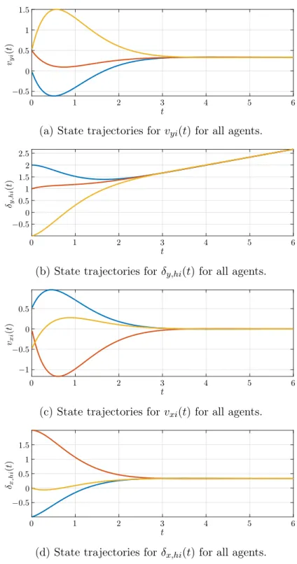
Finally, the state trajectories for this example are shown in Figure 1.17. Figure 1.17a shows that the velocity 𝑣𝑦𝑖(𝑡) achieves consensus around 𝑡 = 4𝑠. Additionally, the state variable 𝛿𝑦,ℎ𝑖(𝑡) in Figure 1.17b also achieves consensus while still varying as a ramp, since it is integrating 𝑣𝑦𝑖(𝑡). The velocity 𝑣𝑥𝑖(𝑡) in Figure 1.17c is also shown to achieve consensus at the same time. Note that 𝛿𝑥,ℎ𝑖(𝑡) in Figure 1.17d achieves consensus, but, differently from 𝛿𝑦,ℎ𝑖(𝑡), has ramp slope close to zero, since 𝑣𝑥𝑖(𝑡) converges to a value close to zero.
1.6
High-order Dynamics
Many agents can be described as high-order integrator dynamics, which is comprised by any input-state linearizable system, e.g. speed control (Xia et al., 2012), and power generators (Rigatos et al., 2014).
vy
i
(
t
)
t
−0.5 0
0 0.5
1
1 1.5
2 3 4 5 6
(a) State trajectories forv𝑦𝑖(t) for all agents.
δy
,h
i
(
t
)
t
−0.5 0
0 0.5
1
1 1.5
2
2 2.5
3 4 5 6
(b) State trajectories forδ𝑦,ℎ𝑖(t) for all agents.
vx
i
(
t
)
t
−1
−0.5 0
0 0.5
1 2 3 4 5 6
(c) State trajectories forv𝑥𝑖(t) for all agents.
δx
,h
i
(
t
)
t
−0.5 0
0 0.5
1
1 1.5
2 3 4 5 6
(d) State trajectories forδ𝑥,ℎ𝑖(t) for all agents.
engine, drive line, brake system, aerodynamics drag, tire friction, rolling resistance, and gravitational force, with the following assumptions extracted from Zheng et al. (2016) (Swaroop et al., 1994; Xiao and Gao, 2011; Li et al., 2011a, 2013):
• The tire longitudinal slip is negligible, and the powertrain dynamics are lumped into a first-order inertial transfer function;
• The vehicle body is considered to be rigid and symmetric;
• The influence of pitch and yaw motions is neglected;
• The driving and braking torques are controllable inputs.
With these considerations, the following simplified but still nonlinear longitudinal dynamics of a vehicle𝑖 can be obtained (Zheng et al., 2016):
˙
𝑠𝑖(𝑡) =𝑣𝑖(𝑡) (1.30)
˙
𝑣𝑖(𝑡) =
1
𝑚𝑖
(︂ 𝜂𝑖
𝑇𝑖(𝑡)
𝑅𝑖 −
𝐶𝑖𝑣𝑖2−𝑚𝑖𝑔𝑓
)︂
(1.31)
𝜄𝑖𝑇˙𝑖(𝑡) +𝑇𝑖(𝑡) =𝑇𝑖,𝑑𝑒𝑠(𝑡), (1.32)
where𝑠𝑖(𝑡),𝑣𝑖(𝑡)denote the position and velocity,𝑚𝑖 is the vehicle mass,𝐶𝑖is the lumped aerodynamic drag coefficient, 𝑔 is the acceleration due to gravity, 𝑓 is the coefficient of rolling resistance, 𝑇𝑖(𝑡) denotes the actual driving/braking torque, 𝑇𝑖,𝑑𝑒𝑠(𝑡) is the desired driving/braking torque,𝜄𝑖is the inertial delay of vehicle longitudinal dynamics,𝑅𝑖denotes the tire radius, and 𝜂𝑖 is the mechanical efficiency of driveline.
Zheng et al. (2016) use the output position to linearize the nonlinear model by making
𝑇𝑖,𝑑𝑒𝑠(𝑡) =
1
𝜂𝑖
(𝐶𝑖𝑣𝑖(2𝜄𝑖𝑣˙𝑖 +𝑣𝑖) +𝑚𝑖𝑔𝑓+𝑚𝑖u𝑖)𝑅𝑖, (1.33)
where u𝑖 is the new input signal after linearization, such that the linear model for the vehicle longitudinal dynamics
𝜂𝑖𝑎˙𝑖(𝑡) +𝑎𝑖(𝑡) = u𝑖(𝑡), (1.34) where 𝑎˙𝑖(𝑡) = 𝑣𝑖(𝑡) denotes the acceleration. Finally, the third-order state space model can be written as (Xiao and Gao, 2011; Zheng et al., 2016)
⎡
⎢ ⎣
˙
𝑠𝑖(𝑡)
˙
𝑣𝑖(𝑡)
˙
𝑎𝑖(𝑡)
⎤ ⎥ ⎦= ⎡ ⎢ ⎣
0 1 0 0 0 1 0 0 −1
𝜄𝑖 ⎤ ⎥ ⎦ ⎡ ⎢ ⎣
𝑠𝑖(𝑡)
𝑣𝑖(𝑡)
𝑎𝑖(𝑡)
⎤ ⎥ ⎦+ ⎡ ⎢ ⎣ 0 0 1 𝜄𝑖 ⎤ ⎥
⎦u𝑖(𝑡). (1.35)
The objective in a platoon problem is to make all vehicles move at the same speed while maintaining a desired inter-vehicle spacing policy. The platoon problem has a long history and has recently attracted extensive research interests. Some overviews can be seen in the works by Tsugawa (2002), Li et al. (2015), and Jia et al. (2016).
A platoon can be viewed as a group of agents, i.e. vehicles, and the problem may be described similarly to the consensus-based formation problem, to achieve consensus on three variables: the distance from the current position to a pre-defined position; the speed; and the acceleration. The following state variables are thus defined
⎡
⎢ ⎣
˜
𝑠𝑖(𝑡)
𝑣𝑖(𝑡)
𝑎𝑖(𝑡)
⎤
⎥ ⎦=
⎡
⎢ ⎣
𝑠𝑖(𝑡)−𝑠*𝑖
𝑣𝑖(𝑡)
𝑎𝑖(𝑡)
⎤
⎥
⎦, (1.36)
with 𝑠*
𝑖 defined similarly to 𝑥*𝑖 in Equation (1.6) for the formation problem. Hence, the vehicles can achieve platoon with a distance policy𝛿𝑖𝑗 as shown in Figure 1.18 which can be defined from𝑠*
𝑖 and 𝑠*𝑗 as
𝛿𝑖𝑗 =𝑠*𝑖 −𝑠
*
𝑗. (1.37)
Figure 1.18 shows an example where each vehicle can measure the distance only to the vehicle in front of itself with𝑎𝑖𝑗 describing these neighboring vehicles.
a43= 1 a32= 1 a21= 1
δ43 = 20m δ32 = 20m δ21= 20m
Figure 1.18: Platooning problem.
A consensus protocol that can drive the agents to consensus is
u𝑖(𝑡) =−
∑︁
𝑗∈𝑁𝑖
𝑎𝑖𝑗(𝛼3(˜𝑠𝑖(𝑡)−𝑠˜𝑗(𝑡)) +𝛼2(𝑣𝑖(𝑡)−𝑣𝑗(𝑡)) +𝛼1(𝑎𝑖(𝑡)−𝑎𝑗(𝑡))), (1.38)
which replacing 𝑠˜𝑖(𝑡) from (1.36) yields
u𝑖(𝑡) = −
∑︁
𝑗∈𝑁𝑖
𝑎𝑖𝑗
(︀
𝛼3(𝑠𝑖(𝑡)−𝑠𝑗(𝑡)−(𝑠*𝑖 −𝑠
*
𝑗)) +𝛼2(𝑣𝑖(𝑡)−𝑣𝑗(𝑡)) +𝛼1(𝑎𝑖(𝑡)−𝑎𝑗(𝑡))
)︀ ,
(1.39)
with 𝛿𝑖𝑗 from (1.37), the consensus protocol can be written equivalently as
u𝑖(𝑡) = −
∑︁
𝑗∈𝑁𝑖
and 𝑠𝑖(𝑡)−𝑠𝑗(𝑡) can be assessed by a sensor located in front of vehicle 𝑖 to measure the distance to vehicle𝑗.
The group of vehicles represented in Figure 1.18 is simulated in order to show the state evolution as the agents achieve platoon formation. The agents are indexed as follows, the rightmost red vehicle is agent1, the green is agent 2, the blue one is agent 3, and finally agent 4 refers to the leftmost yellow car. The desired distance between each pair of cars is𝛿43=𝛿32=𝛿21= 20m.
Note that the red vehicle receives no information from any other agent and therefore is considered the leader. Its velocity thus remains constant, as the control input from the consensus protocol is zero. Additionally, all the agents are expected to achieve consensus on the velocity and acceleration defined by the leader.
The initial conditions are considered as follows: 𝑠1(0) = 200m,𝑠2(0) = 150m,𝑠3(0) =
90m, and 𝑠4(0) = 20m are the initial positions in relation to an inertial reference; all the initial velocities are considered to be 𝑣1(0) = 𝑣2(0) = 𝑣3(0) = 𝑣4(0) = 10m/𝑠; and all the accelerations are considered initially null, i.e 𝑎1(0) =𝑎2(0) =𝑎3(0) = 𝑎4(0) = 0m/𝑠2. For the spacing distances defined as 𝛿43=𝛿32 =𝛿21 = 20m, it can be defined the desired formation-like parameters as 𝑠*
1 = 60m,𝑠*2 = 40m,𝑠*3 = 20m, and𝑠*4 = 0m.
A simulation is carried-out to show that the analysis of the vehicle dynamics (1.35) with the consensus protocol (1.38) can be applied to guarantee platoon considering gains
𝛼1 = 1, 𝛼2 = 2, and 𝛼3 = 1 as designed by Zheng et al. (2016). Figure 1.19 shows the evolution of the space distance between two adjacent cars. The simulation carried out shows that the vehicles manage to achieve the desired distance of 20m between the cars.
si
(
t
)
−
si−
1
(
t
)
t
2 4 6 8 10 12 14 16 18
0 0 20
20 40
60 80
Figure 1.19: Spacing between the vehicles for𝑖= 1,2,3.
˜
si
(
t
)
t
0 2 4 6 8 10 12 14 16 18 20 50
100 150 200 250 300
(a) State trajectories fors˜𝑖(t) =s𝑖(t)−s*𝑖 for all agents.
vi
(
t
)
t
0 2 4 6 8 12 14 16 18 10
10 20
20 30
40 50
(b) State trajectories forv𝑖(t) for all agents.
ai
(
t
)
t 0
0 2 4 6 8 12 14 16 18
−10 10
10 20
20 30
(c) State trajectories for a𝑖(t)for all agents.
Figure 1.20: State trajectories for vehicles longitudinal dynamics.
and constant in Figure 1.20b, and𝑠˜𝑖(𝑡)varying as a ramp with slope given by the velocity in Figure 1.20a.
1.7
Overview of this Thesis and Contributions
In Chapter 2, it is presented a transformation that allows consensus problems with communication and input delays to be analyzed as stability problems. Additional lemmas used throughout this thesis are also presented in that chapter.
An analysis of the impacts of delays in communication or input-delays will be presented in Chapter 3 showing that for different values of constant time-delays, the introduction of the delays can either prevent or enable consensus. It shows the importance of analyzing delays in different intervals of variation. The presented results are exact, i.e. necessary and sufficient. Part of these results were published by Savino et al. (2015) and are also applied here to communication delays.
Next, results considering the analysis of consensus with the considered bounds of time-varying delays is presented in Chapter 4. The presented results are sufficient but less conservative than others in the literature. This chapter generalizes the results published by Savino et al. (2013), Savino et al. (2014b), Savino et al. (2014a), and Savino et al. (2016b), and extends the results to the application in communication delays.
Analysis of switching topologies, which can be due to failures in the communication channels causing the drop of communication links, is presented in Chapter 5. This is a reprint of the result published by Savino et al. (2016a), which also generalizes dos Santos Junior et al. (2014) and dos Santos Junior et al. (2015). The result is also applied to communication delays.
The design of the coupling strengths between the agents related to the weights 𝑎𝑖𝑗 assigned to the communication links is presented in Chapter 6. These results are presented by Savino et al. (2016c), a book chapter to be published on the series of Advances in Delays and Dynamics, edited by Springer.
An analysis of single-order consensus applied to rigid bodies with an application in cooperative robotics is shown in Chapter 7. It summarizes the results obtained during the exchange program at the Interactive Robotics Groups in the Massachusetts Institute of Technology. These results follow the lines of the work published by Brito et al. (2015).
Finally, the text ends with the conclusions.
The contributions of this Thesis are summarized next:
for high-order dynamics in Section 2.2, which gives the disagreement systems (2.49) for communication delays and (2.72) for input delays.
• The analysis of consensus on intervals of time-delays for agents described by chain of integrators in Theorem 3.1 for communication and Theorem 3.2 for input de-lays. It is also shown that a multiagent system with agents given by single-order integrator can achieve consensus independent of the communication delay (Corol-lary 3.1), as expected from previous results in the literature. The system can also be independent of the communication delay for second-order integrator dynamics if the gains in the consensus protocol are properly adjusted (Corollary 3.2), and for higher-order the delays can either improve or degrade the systems behavior accord-ing to the interval of time-delay, accordaccord-ing to Theorem 3.1. Likewise, the effects of input-delays always degrade the systems performance for first- and second-order integrators, showing an upper bound for the delay margins in Corollaries 3.3 and 3.4, respectively. For higher-orders, like the communication delays, input delays can also improve or degrade performance according to its interval (Theorem 3.2). This analysis shows that the impact of time-delays, either allowing or preventing consen-sus, depends on the interval on which the time-delay belongs. Thus, consensus with time-delays have to be analyzed on intervals, which is the assumption made for the domain of the time-delays in the next results.
• An LMI method for the analysis of consensus with time-delays is presented for both communication and input delays in Theorem 4.1. The delays are assumed to belong to an interval described by a lower and upper bound in order to analyze the delays on intervals. The result also presents a guaranteed exponential convergence rate for consensus and is related to the time needed to approach consensus. The proposed method is shown to perform better than related results in the literature.
• An extension of the analysis method to deal with switching topologies is presented and a sufficient condition to show consensus is given in Theorem 5.1. The switching behavior is described as a Markov Chain with uncertain parameters, which can describe uncertainties in the model of the transition rates, and also consider time-delays given on intervals.
• The design of the coupling strengths is done with LMI methods in order to increase performance according to a convergence rate in Theorem 6.1, for fixed topologies. It can also be applied to allow greater margins of time-delays, as presented for switching topologies in Theorem 6.2.
Background for Analyzing Consensus
as Stability
This chapter presents how to transform a consensus problem into a stability one, which is necessary for the development of the results to be presented in the following chapters. The representation of the network topology with graphs is followed by the description of the dynamics of multiagent systems with communication delays, input delays, and free of delay as a special case. The chapter is finished with some important lemmas.
2.1
Algebraic Graph Theory
The information flow of a multiagent system is modeled using the algebraic theory of graphs as first proposed by Fax and Murray (2002) and Jadbabaie et al. (2003). An ex-ample of this representation has been introduced in the previous chapter (see Figure 1.2). A more detailed example is presented here in Figure 2.1a, where an undirected graph is used to model the interactions of four agents. An undirected graph refers to commu-nication networks with two-way commucommu-nication links, i.e. if node 1 is able to receive information from node 2, then node 2 also receives information from node 1, and the same is valid for all the other nodes in Figure 2.1a. Additionally, in undirected networks, the coupling strengths 𝑎𝑖𝑗, equivalent to the weights associated to each neighbor𝑗 of an agent 𝑖, obey 𝑎𝑖𝑗 =𝑎𝑗𝑖.
An undirected network is a special case of a directed network, presented in Figure 2.1b. In a directed network, it is not necessary for two agents sharing a link to have bidirectional communication. As seen in Figure 2.1b, node2receives information from node3, but the opposite is not true. The same happens for the links between nodes 3 and 4, and nodes
4 and 2. The two-way communication link as in undirected networks is still possible, as shown for nodes 1 and 2, but, it is not necessary that the two coupling strengths to be
1
2
3
4
a12=a21= 1 a
32=
a23= 1
a42= a24
= 1
a34=a43= 1
(a) Undirect graph.
1
2
3
4
a21= 1
a12= 2
a23= 1
a42= 1
a34= 1
(b) Directed graph.
Figure 2.1: Example of graphs.
equal, e.g. 𝑎21 = 1 and 𝑎12 = 2.
This text makes use of directed graphs, which can also represent undirected graphs. Additionally, directed graphs can also model leader-following multiagent systems. This is the case if𝑎12= 0 in Figure 2.1b, which implies that agent1receives no information from any other agent. An example of a leader following system was presented for platooning in Figure 1.18.
A simple directed graph is denoted by 𝒢(𝒱,ℰ,𝒜), where 𝒱 represents the set of 𝑚
vertices (or nodes) ordered and labeled as 𝑣1, ..., 𝑣𝑚 ∈ 𝒱, ℰ represents the set of directed edges connecting the nodes and dictating the direction of the information flow, given by
𝑒𝑖𝑗 = (𝑣𝑖, 𝑣𝑗), where the first element 𝑣𝑖 is the parent node (tail) and the second element
𝑣𝑗 is the child node (head). No multiple edges or graph loops are allowed. The Adjacency Matrix𝒜 = [𝑎𝑖𝑗] associated with graph 𝒢 assigns a real non-negative value to each edge
𝑒𝑖𝑗, according to
𝑎𝑖𝑗
{︃
= 0, if 𝑖=𝑗 or∄ 𝑒𝑗𝑖,
>0, if and only if ∃ 𝑒𝑗𝑖.
(2.1)
Additionally, it is defined the Degree Matrix𝒟 = [𝑑𝑖𝑖], a diagonal matrix with elements
𝑑𝑖𝑖=
∑︀𝑚
𝑗=1𝑎𝑖𝑗. Given the definitions of the Adjacency and Degree matrices, it follows the definition of the Laplacian Matrix:
𝐿=𝒟 − 𝒜, (2.2)