Reply: Birnbaum's (2012) statistical tests of independence have unknown Type-I error rates and do not replicate within participant

(1)

Reply: Birnbaum’s (2012) statistical tests of independence have

unknown Type-I error rates and do not replicate within participant

Yun-shil Cha

∗

_{Michelle Choi}

†

_{Ying Guo}

†

_{Michel Regenwetter}

†

_{Chris Zwilling}

†

Abstract

Birnbaum (2011, 2012) questioned the iid (independent and identically distributed) sampling assumptions used by state-of-the-art statistical tests in Regenwetter, Dana and Davis-Stober’s (2010, 2011) analysis of the “linear order model”. Birnbaum (2012) cited, but did not use, a test of iid by Smith and Batchelder (2008) with analytically known properties. Instead, he created two new test statistics with unknown sampling distributions.

Our rebuttal has five components: 1) We demonstrate that the Regenwetter et al. data pass Smith and Batchelder’s test of iid with flying colors. 2) We provide evidence from Monte Carlo simulations that Birnbaum’s (2012) proposed tests have unknown Type-I error rates, which depend on the actual choice probabilities and on how data are coded as well as on the null hypothesis of iid sampling. 3) Birnbaum analyzed only a third of Regenwetter et al.’s data. We show that his two new tests fail to replicate on the other two-thirds of the data, within participants. 4) Birnbaum selectively picked data of one respondent to suggest that choice probabilities may have changed partway into the experiment. Such nonstationarity could potentially cause a seemingly good fit to be a Type-II error. We show that the linear order model fits equally well if we allow for warm-up effects. 5) Using hypothetical data, Birnbaum (2012) claimed to show that “true-and-error” models for binary pattern probabilities overcome the alleged short-comings of Regenwetter et al.’s approach. We disprove this claim on the same data.

Keywords: binary choice models, true-and-error models, iid sampling, statistical testing.

1 Introduction.

Imagine that you are offered the choice between two wheels of chance, as displayed in Figure 1. The chosen wheel of chance, in such a gamble pair, if played for real

The authorship of this paper is alphabetical. Analyzing the same data several times can be problematic because it may over-utilize the degrees of freedom available and it may lead to selection biases in pub-lication. To avoid publication bias, the authors and the Regenwetter lab-oratory did not carry out any tests of iid sampling assumptions on the Regenwetter et al. (2011) data other than those reported in this paper. The authors also did not inspect any data of Regenwetter et al. (2011) other than Birnbaum’s (2012) Table 2, to inform their hypotheses or analyses. This means that the correct number of degrees of freedom for Participant 2, Cash I, is unknown for the reduced data sets where 4 trials are dropped. No other analyses are affected by the data in-spection. We thank Jason Dana, Clintin Davis-Stober, Marc Jekel, A. A. J. Marley, and Anna Popova, for critical comments on earlier ver-sions, as well as Greg Francis and Uri Simonsohn for useful references. This work was supported by National Science Foundation grants SES-DRMS # 08-20009 (PI: M. Regenwetter) and SES-SES-DRMS # 1062045 (PI: M. Regenwetter), and by an Arnold O. Beckman Research Award (PI: M. Regenwetter), awarded by the University Research Board of the University of Illinois at Urbana-Champaign. Any opinions, find-ings, and conclusions or recommendations expressed in this publication are those of the authors and do not necessarily reflect the views of col-leagues, the National Science Foundation, the Korea Institute of Public Finance, or the University of Illinois. Address: Michel Regenwetter, Department of Psychology, 603 E. Daniel St., Champaign, IL 61820. Email: regenwet@illinois.edu

∗_{Korea Institute of Public Finance} †_{University of Illinois at Urbana-Champaign}

money, will be spun. If the black part of the wheel is oriented towards the Dollar amount when it stops (which is the case in both wheels as displayed in Figure 1) then you win the indicated amount, otherwise nothing. In the left gamble of Figure 1 you can win $25.2 (with 37.5% chance), whereas in the right gamble you can win $22.4 (with 48.8% chance). As the screenshot shows, the nu-merical probabilities of winning are not provided. The decision maker depends on the relative size of the black shaded area to evaluate the chance of winning. When offered such stimuli repeatedly, decision makers tend to fluctuate in the choices they make. For over 50 years, it has been a point of debate how one can model choice vari-ability formally. A natural approach is to model choice behavior probabilistically.

Regenwetter, Dana and Davis-Stober (2010, 2011) [henceforth RDDS] investigated a mathematical model of binary choice probabilities with a distinguished his-tory in economics, operations research, and psychology, whose mathematical structure has been studied intensely over several decades (see, e.g., Becker, DeGroot, & Marschak; 1963, Block & Marschak, 1960, Bolotashvili, Kovalev, & Girlich, 1999; Cohen & Falmagne, 1978, 1990; Fiorini, 2001; Fishburn, 1992; Fishburn & Fal-magne, 1989; Gilboa, 1990; Grötschel, Jünger & Reinelt, 1985; Heyer & Niederée, 1992; Koppen, 1991, 1995; Marschak, 1960), but for which there did not

(2)

Figure 1: Screen shot of a Cash I paired-comparison stim-ulus (see also RDDS, Figure 2)

ously exist an appropriate statistical test. This model has been studied under several labels, including “binary choice model”, “linear ordering polytope”, “random pref-erence model”, “random utility model” and “rationaliz-able model of stochastic choice”, and it has been stated in several different mathematical forms that make the same empirical predictions (see, e.g., Fishburn, 2001; Regen-wetter & Marley, 2001). We will refer to it as thelinear order model. According to this model, preferences form a probability distribution over linear orders, i.e., over rank-ings without ties. The probability that a person chooses one gamble over another is the probability that s/he ranks the chosen gamble higher than the non-chosen gamble.

Denote the probability that a person choosesx(say, the

left gamble in Figure 1) overy(say, the right gamble in

Figure 1) asPxy. The linear order model makes

restric-tive predictions: It requires that thetriangle inequalities

hold, according to which, for all distinct choice options

a, b, c,

Pab+Pbc−Pac≤1. (1)

This model has a particular mathematical form that long eluded statistical testing: For inequality constraints like these, standard likelihood ratio tests are not applicable, goodness-of-fit statistics need not satisfy the familiar

asymptoticχ2

(Chi-squared) distributions, and it is not even meaningful to count parameters (e.g., binary choice probabilities) to obtain degrees of freedom of a test. For-mally adequate statistical tests for such models have been discovered only recently (Davis-Stober, 2009). Regen-wetter, Dana and Davis-Stober (2010, 2011) were the first to carry out such a state-of-the-art “order-constrained” test of the linear order model. Even breakthrough re-sults come at a price: To our knowledge, there does cur-rently not exist a statistical test for the triangle

inequali-ties that does not assume iid (independent and identically

distributed) sampling of empirical observations.

Notice that the triangle inequalities (1) make no men-tion of time, of the individual making these choices, or of repeated observations. They do not require binary

choice probabilities to remain constant over time or be the same for different decision makers (i.e., they do not require an identical distribution), nor do they require bi-nary choices to be made stochastically independently of each other (see Regenwetter, submitted, for a thorough discussion). Birnbaum (2011, 2012) [henceforth MB] has questioned the iid sampling assumption used by RDDS’s statistical test and recommended his own models, the so called “true-and-error” models, as an alternative. Regen-wetter (submitted) shows that MB is mistaken to attribute the iid assumption to the linear order model itself, i.e., to the triangle inequalities (1). Among the leading models of probabilistic choice, the linear order model stands out in being invariant under non-stationary choice probabili-ties (i.e., invariant under certain violations of the “iden-tically distributed” part of “iid”). Regenwetter (submit-ted) also shows that, in contrast, a number of published papers on “true-and-error” models do, in fact, require bi-nary choice to be iid in both the model formulation and in the statistical test.

The main concern in this paper, however, is with Birn-baum’s (2012) claim that the iid assumption, used by the state-of-the-art test in RDDS, is violated in the RDDS data. We will first provide a brief introduction to the RDDS experiment, then show that the RDDS data pass a well-known test of iid sampling without a hitch. We then document that Birnbaum’s (2012) proposed tests of iid sampling have unknown Type-I error rates that even ap-pear to change with the way in which binary choices are coded, and do not actually appear to test iid sampling per se. We add to this conclusion the finding that Birnbaum’s (2012) tests fail to replicate within participant. We pro-vide epro-vidence against MB’s suggestion that the excellent model performance in RDDS might be a Type-II error in which warm-up effects could have made binary choice probabilities shift early in the experiment and then choice probabilities violating the model could have accidentally averaged to satisfy the triangle inequalities. Last but not least, we use Birnbaum’s own (2012) hypothetical data to disprove MB’s claim that “true-and-error” models over-come alleged limitations of the linear order model.

2 The experiment of RDDS.

(3)

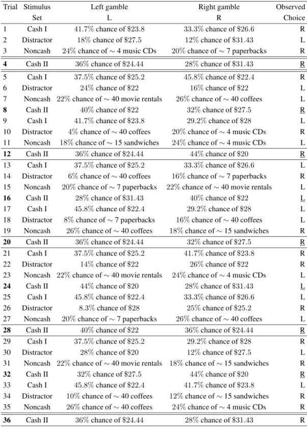
Table 1: First 36 out of 800 pairwise choices of Participant # 100 in RDDS.

Trial Stimulus Left gamble Right gamble Observed

Set L R Choice

1 Cash I 41.7%chance of$23.8 33.3%chance of$26.6 R

2 Distractor 18%chance of$27.5 12%chance of$31.43 L

3 Noncash 24%chance of∼4 music CDs 20%chance of∼7 paperbacks R

4 Cash II 36%chance of$24.44 28%chance of$31.43 R

6 Distractor 24%chance of$22 16%chance of$22 L

7 Noncash 22%chance of∼40 movie rentals 26%chance of∼40 coffees L

8 Cash II 40%chance of$22 32%chance of$27.5 R

9 Cash I 41.7%chance of$23.8 29.2%chance of$28 L

10 Distractor 4%chance of∼40 coffees 20%chance of∼4 music CDs R

11 Noncash 18%chance of∼15 sandwiches 24%chance of∼4 music CDs L

12 Cash II 36%chance of$24.44 44%chance of$20 R

13 Cash I 37.5%chance of$25.2 33.3%chance of$26.6 L

14 Distractor 6%chance of∼40 coffees 16%chance of∼7 paperbacks R

15 Noncash 20%chance of∼7 paperbacks 22%chance of∼40 movie rentals L

16 Cash II 28%chance of$31.43 40%chance of$22 L

17 Cash I 45.8%chance of$22.4 29.2%chance of$28 L

18 Distractor 8%chance of∼7 paperbacks 16%chance of∼40 coffees L

19 Noncash 26%chance of∼40 coffees 18%chance of∼15 sandwiches R

22 Distractor 14%chance of$22 26%chance of$22 R

23 Noncash 22%chance of∼40 movie rentals 24%chance of∼4 music CDs L

24 Cash II 44%chance of$20 28%chance of$31.43 L

26 Distractor 8.3%chance of$28 25%chance of$25.2 R

27 Noncash 20%chance of∼7 paperbacks 26%chance of∼40 coffees L

28 Cash II 40%chance of$22 36%chance of$24.44 R

29 Cash I 37.5%chance of$25.2 29.2%chance of$28 R

30 Distractor 28%chance of$20 12%chance of$27.5 L

31 Noncash 22%chance of∼40 movie rentals 18%chance of∼15 sandwiches R

32 Cash II 32%chance of$27.5 44%chance of$20 R

34 Distractor 10%chance of∼40 coffees 12%chance of∼15 sandwiches R

35 Noncash 26%chance of∼40 coffees 24%chance of∼4 music CDs R

Note: The symbol∼stands for “approximately”.

one in Figure 1. The 400 pairwise choices were spread over five weekly test sessions of 80 choices each. RDDS

(4)

com-puter. They considered three distinct sets of 5 lotteries, as well as some Distractor items. Their Cash I set was the contemporary dollar equivalent of Tversky’s (1969) stim-uli, whereas their Cash II and Noncash stimulus sets were new. Like Tversky (1969) they presented each lottery pair 20 times (except for the Distractors, which varied).

Table 1 gives an example summary of the first 36

tri-als of the RDDS experiment1_{for Participant}_#100_{. On}

Trial 1, the decision maker faced the choice between a

“41.7%chance of winning$23.8” (presented as a wheel

of chance on the left side of the screen) and a “33.3%

chance of winning$26.6” (presented on the right side).

This was a stimulus from the Cash I set. The decision maker chose the gamble presented on the right. On Trial 2, the decision maker was presented with the first of 200 Distractor items, which were intended to interfere with the memory of earlier choices, thus making it difficult to recognize repeated items. Trial 3 involved gambles for

non-cash prizes, namely a “24%chance of winning a gift

certificate worth approximately 4 music CDs” or a “20%

chance of winning a gift certificate for approximately 7 paperback books”.

In Table 1, Trials 4, 12, 20, 28, and 36 are set apart

by horizontal lines. The lottery with a “36%chance of

winning$24.44” was presented in each of these five

tri-als. The side of the screen on which each lottery appeared was randomized. The lottery presentation, unbeknownst to the participant, cycled through the four stimulus sets in the order Cash I, Distractor, Noncash, Cash II. The pair of lotteries presented in a given trial was picked randomly from its stimulus set with the constraint that it had not ap-peared in the previous five trials from that set; and each individual lottery was chosen with the constraint that it had not appeared in the previous trial from that set. This

is why the trials involving a “36% chance of winning

$24.44” are separated by at least eight pairwise choices,

and why the repetition of the lottery pair in Trial 4 did not occur until at least 24 trials later; in this case, it was in Trial 36.

Many prominent probabilistic models of choice in the behavioral and economic sciences, including the models

that Tversky (1969) considered,2 _{assume that the}

deci-sion maker has a single fixed deterministic preference state throughout the experiment and that variability in observed choices is due to noise or error in one form

1_{These followed an initial set of 18 trials, not shown in the table,}

designed to familiarize the participant with the task.

2_{Tversky attempted to reject weak stochastic transitivity in favor of}

a modal choice model of a lexicographic semiorder. See Regenwetter (submitted) for an explanation and mathematical proofs about what is allowed to vary and what is required to be fixed, in such models, as well as the role of independence assumptions in these models and in statistical tests of these models. See Iverson and Falmagne (1985) and RDDS for an explanation why Tversky’s (1969) attempt did not suc-ceed, despite hundreds of citations of Tversky’s paper reporting that it succeeded.

or another (Becker et al., 1963; Birnbaum, 2004; Block & Marschak, 1960; Carbone & Hey, 2000; Harless & Camerer, 1994, 1995; Hey, 1995, 2005; Hey & Car-bone, 1995; Loomes, 2005; Loomes, Moffatt & Sug-den, 2002; Loomes, Starmer & SugSug-den, 1991; Loomes & Sugden, 1995, 1998; Luce, 1959; Luce & Suppes, 1965; Marschak, 1960; Tversky, 1969). The linear order model tested in RDDS models preferences themselves as proba-bilistic. For example, a decision maker could be uncertain about what he or she prefers on a given trial.

The statistical test currently available for such mod-els requires that one can combine multiple observations together to estimate choice probabilities from choice pro-portions:

1. Writing x for the lottery with a “36% chance of

winning$24.44” andy for the lottery with a “28%

chance of $31.43,” the statistical test in RDDS

treated Trials 4 and 36 as two independent draws from a single underlying Bernoulli process with

probabilityPxyof choosingxovery.

2. Similarly, for two lottery pairs, say,xversusyanda

versusb, from the same stimulus set (thus separated

by at least 4 trials), the statistical test assumed that those two binary choices were independent draws

from two Bernoulli processes with probabilitiesPxy

andPab.

Because each stimulus set was analyzed separately, there was no assumption about the relationship between choices from different stimulus sets, say, the choices made on Trials 1 and 2, for instance. The iid assumptions applied only to choices within stimulus set. These two assumptions allow a researcher to use choice proportions as estimators of choice probabilities and this is precisely how they are routinely used in quantitative analyses of probabilistic choice models in psychology, econometrics, and related disciplines. It is the first iid sampling assump-tion above that MB has quesassump-tioned. Birnbaum (2012) claims that this iid assumption is violated in the RDDS data. We will now consider the legitimacy of that infer-ence.

3 A test of iid sampling suggested in

Smith and Batchelder (2008).

(5)

Let(i, i′₎_{denote some gamble pair. Throughout this}

section, we will enumerate only the 20 trials that the

gam-ble pair(i, i′₎_{was presented in RDDS (not the 800}

tri-als of their experiment). So, Tritri-als 4 and 36 in Table

1 becomet = 1andt = 2 for the gamble pair(i, i′₎

wherei:“36%chance of$24.44” andi′_{: “}_28%_{chance of}

$31.43”. Fort∈ {1,2, . . . ,20}, let

Xit=

  

 

1 if the decision maker chooses

alternative ion trialt,

0 otherwise.

We wish to test, for each gamble pair(i, i′₎_{, whether}

the Xit result from 20 independent and identically

dis-tributed Bernoulli trials, fort = 1,2, . . . ,20. By Smith and Batchelder (2008, p. 727), we can consider the fol-lowing quantity defined in their Eq. 21, which checks for a 1-step choice reversal from trialtto trialt+ 1:

Ait=

(

1, ifXi,t6=Xi,t+1,

0, otherwise.

Based on this quantity, we consider the number of 1-step choice reversals given by

Ai= 19 X

t=1

Ait. (2)

By Smith and Batchelder (2008), if the 20 Bernoulli tri-als are independent and identically distributed, i.e., have

fixed probabilityθiof success, we must have

E(Ai) = 38θi(1−θi). (3)

We give a proof in the Appendix. Smith and Batchelder

(2008) did not provide a standard error forAi. We show

in the Appendix that the standard error equals

SE(Ai) =

q

38θi(1−θi) 1−2θi(1−θi)

. (4)

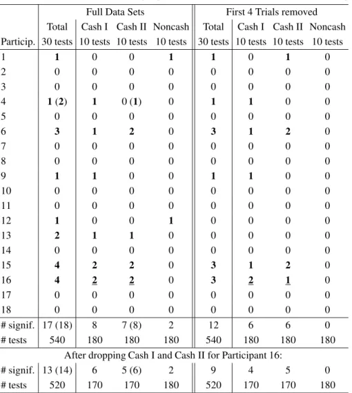
Table 2 shows the results of this test when applied to the RDDS data. For each of the 18 participants in Re-genwetter et al. (2011), we carried out 30 tests (for the 30 binomials that RDDS use for each person, 10 for each of Cash I, Cash II, and Noncash) to see whether we may assume, for each of the 30 gamble pairs, iid draws from a fixed Bernoulli process to obtain 30 distinct binomials per respondent. This analysis of iid sampling involved a total of18×30 = 540hypothesis tests.3_{We determined}

confi-dence intervals using the point estimate given in our Eq. 3 and the standard error,SE(Ai)given in our Eq. 4. We

re-port the number of significant violations (marked inbold)

3_{Besides a full analysis of all data sets, the table also provides an}

analysis for the reduced data sets where we dropped the first four trials for each participant and for each gamble pair. We provide the rationale for this analysis later. Table 2 shows no major changes when we drop the first four trials.

using a margin of error of2SE(Ai), or1.96SE(Ai)

(re-ported in parentheses, when different).

Since we are looking for evidence of mistaken accep-tance of the linear order model in RDDS, we also provide an analysis where we leave out the two data sets (Cash I & II, Participant 16) where Regenwetter et al. (2011) already rejected the linear order model (underlined). Re-jections by Smith and Batchelder’s (2008, Eq. 21) test

occurred at a rate of∼3%, well within standard Type I

error range. There is no reason to conclude, based on this test, that the binary choices of each individual in Regen-wetter et al.’s (2011) data were anything but independent and identically distributed Bernoulli trials, hence that the choice frequencies originated from anything but Binomi-als. The null hypothesis of iid sampling in RDDS is re-tained in this hypothesis test.

4 Type-I error rates of Birnbaum’s

(2012) tests.

In contrast to Smith and Batchelder’s test statistic, whose expected value and standard error we reviewed above, Birnbaum (2012) created two new test statistics with un-known sampling distributions. Using these new

statis-tics, Birnbaum (2012) estimated two quantitiespνandpr

from the data and, without formal proof, interpreted these

quantitiespν andpras p-values of tests of iid sampling

for a given participant in RDDS. Birnbaum concluded that a data set in RDDS violates the iid assumption “sig-nificantly” (at anαlevel of 0.05) whenpν < 0.05,

re-spectively, whenpr<0.05.

To better understand Birnbaum’s test statistics, we can borrow tools from an ongoing debate in the behavioral, statistical, and medical sciences. That debate is primarily concerned about “publication bias”, “p-hacking”, “data peeking”, the “file drawer problem”, etc. (Francis, 2012a, 2012b; Ioannidis & Trikalinos, 2007; Macaskill, Walter & Irwig, 2001; Simmons, Nelson & Simonsohn, 2011). We tap into some of the tools with which this literature investigates whether reported p-values match what is ex-pected for a given set of hypotheses and a given effect size. Specifically, we build on the fact that p-values are, themselves, random variables (Murdoch, Tsai & Adcock, 2008). The p-values of a continuous statistic must satisfy a uniform distribution under the null hypothesis, whereas the p-values of finite statistics can display more compli-cated behavior (Gibbons & Pratt, 1975; Hung, O’Neill, Bauer & Kohne, 1997; Murdoch et al., 2008). We will

consider the distribution of Birnbaum’s (2012)pν- and

pr-values. In particular, we use Monte Carlo simulation

(6)

Table 2: Test of iid binary choice following Eq. 21 and text in Smith and Batchelder (2008, p. 727).

Full Data Sets First 4 Trials removed

Total Cash I Cash II Noncash Total Cash I Cash II Noncash

Particip. 30 tests 10 tests 10 tests 10 tests 30 tests 10 tests 10 tests 10 tests

1 1 0 0 1 1 0 1 0

2 0 0 0 0 0 0 0 0

3 0 0 0 0 0 0 0 0

4 1(2) 1 0 (1) 0 1 1 0 0

5 0 0 0 0 0 0 0 0

6 3 1 2 0 3 1 2 0

7 0 0 0 0 0 0 0 0

8 0 0 0 0 0 0 0 0

9 1 1 0 0 1 1 0 0

10 0 0 0 0 0 0 0 0

11 0 0 0 0 0 0 0 0

12 1 0 0 1 0 0 0 0

13 2 1 1 0 0 0 0 0

14 0 0 0 0 0 0 0 0

15 4 2 2 0 3 1 2 0

16 4 2 2 0 3 2 1 0

17 0 0 0 0 0 0 0 0

18 0 0 0 0 0 0 0 0

# signif. 17 (18) 8 7 (8) 2 12 6 6 0

# tests 540 180 180 180 540 180 180 180

After dropping Cash I and Cash II for Participant 16:

# signif. 13 (14) 6 5 (6) 2 9 4 5 0

# tests 520 170 170 180 520 170 170 180

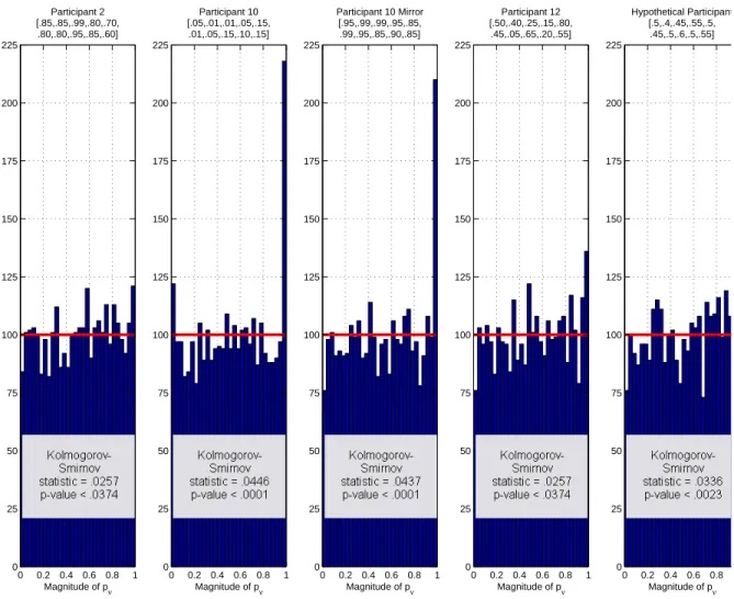
Figures 2 and 3 show five histograms for the

distribu-tion ofpν-values andpr-values (computed separately for

pν andpr) for five different sets of binary choice

prob-abilities. Each histogram tallies the distribution of p

-values for 3,000 simulated iid samples.4_{In each case, we}

expect 100p-values per bin under the null hypothesis, as

indicated by the horizontal line. Even for 3,000 simulated

iid samples, the actual observed numbers ofp-values in

each bin varies substantially around that expected

num-ber. For pν in Figure 3, a Kolmogorov-Smirnoff test

comes out significant in each histogram, suggesting that

thepν-values are not uniformly distributed as they should

be if we treat the underlying statistic as a continuous ran-dom variable. Furthermore, it appears that the

distribu-4_{Our Table 5 shows that we replicated the value of}_p

ν(using only 10,000 pseudo-random permutations to save computation time) that Birnbaum (2012) provided for Cash I (using 100,000 permutations). Even running the Monte Carlo simulation with 10,000 pseudo-random permutations per run used up months of computer time.

tion ofpν-values is different for different choice

proba-bilities, even though in each case, the data were simu-lated via the null hypothesis of iid sampling. The

distri-bution ofpν-values appears to reflect other properties of

the data, not just whether or not iid holds.5 _{In Figure 3,}

a Kolmogorov-Smirnoff test comes out significant in one of the five cases, suggesting that thepr-values in question

are not uniformly distributed as they should be under the null hypothesis.

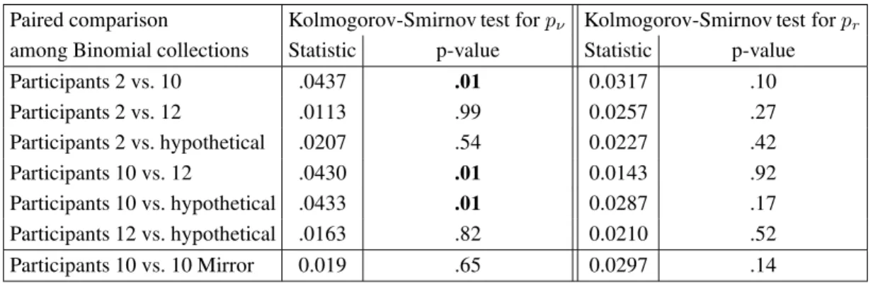
Table 3 provides comparisons of the simulated

sam-pling distributions forpν andpr among pairs of

bino-mial collections that generated the iid data. For the

comparison of the simulated sampling distributions, the Kolmogorov-Smirnov test finds the three pairs differ

sig-nificantly from each other forpν. The corresponding test

forprdid not yield any significant disagreements among

5_{The Smith and Batchelder test explicitly accounts for binary choice}

(7)

Figure 2: Illustrative analysis of the sampling distribution ofpν approximated through 3,000 simulated iid data sets

using the maximum likelihood binomial parameters of three participants from Regenwetter et al. (2011) Cash I, and a hypothetical participant. The underlying binomial probabilities are given above the histograms. The expected frequency in each bin under the uniform null is given by the horizontal line. The Kolmogorov-Smirnov statistic is significant in each case, i.e., each distribution differs significantly from a uniform on[0,1].

Magnitude of p_ν

ν

Participant 2 [.85,.85,.99,.80,.70,

.80,.80,.95,.85,.60]

0 0.2 0.4 0.6 0.8 1 0

25 50 75 100 125 150 175 200 225

Magnitude of p_ν Participant 10 [.05,.01,.01,.05,.15, .01,.05,.15,.10,.15]

0 0.2 0.4 0.6 0.8 1 0

25 50 75 100 125 150 175 200 225

Magnitude of p_ν Participant 10 Mirror

[.95,.99,.99,.95,.85, .99,.95,.85,.90,.85]

0 0.2 0.4 0.6 0.8 1 0

25 50 75 100 125 150 175 200 225

Magnitude of p_ν Participant 12 [.50,.40,.25,.15,.80,

.45,.05,.65,.20,.55]

0 0.2 0.4 0.6 0.8 1 0

25 50 75 100 125 150 175 200 225

Magnitude of p_ν Hypothetical Participant

[.5,.4,.45,.55,.5, .45,.5,.6,.5,.55]

0 0.2 0.4 0.6 0.8 0

25 50 75 100 125 150 175 200 225

simulated sampling distributions, even though Figure 3 suggests a deviation from uniformity for the sampling

distribution forpron data simulated from the collection

of binomials that best fits Participant 10 in Cash I of

RDDS. This makes the analysis forpr somewhat more

ambiguous.

In each histogram of Figures 2 and 3, the left tail of the distribution is of utmost importance, because it shows how often one will observe small p-values when the null hypothesis holds. This means that the left tail of the his-togram gives an idea of Type-I error rates: A spike in the left tail suggests that the Type-I error rate is higher than it should be, because there are too many small p-values. A trough in the left tail suggests a conservative test because there are not enough small p-values to reject the null at a

rate ofαwhen we use a significance level ofα.

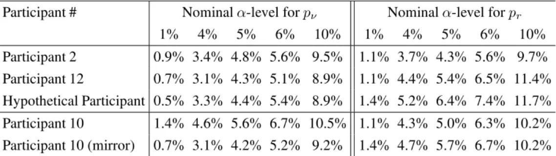
The requirement that a p-value be uniformly dis-tributed under the null hypothesis applies only for con-tinuous statistics. However, the novel statistics

underly-ingpν andpr can, in fact, only take finitely many

dif-ferent values in data like those in RDDS. Therefore, it may be more informative to compare nominal Type-I er-ror rates (α) with the actual rates of false rejection, for various nominal Type-I error rates when analyzing data sets that we know to be iid. We report this in Table 4. There appears to be little rhyme or reason to the actual

Type-I error rates. Forpν, the test appears to be

(8)

Table 3: Comparison of simulated sampling distributions forpν andprfor different collections of binomials.

Paired comparison Kolmogorov-Smirnov test forpν Kolmogorov-Smirnov test forpr

among Binomial collections Statistic p-value Statistic p-value

Participants 2 vs. 10 .0437 .01 0.0317 .10

Participants 2 vs. 12 .0113 .99 0.0257 .27

Participants 2 vs. hypothetical .0207 .54 0.0227 .42

Participants 10 vs. 12 .0430 .01 0.0143 .92

Participants 10 vs. hypothetical .0433 .01 0.0287 .17

Participants 12 vs. hypothetical .0163 .82 0.0210 .52

Participants 10 vs. 10 Mirror 0.019 .65 0.0297 .14

“failure” the test6is no longer conservative, even though

these binary choice probabilities are the same and differ only by how pairwise choices are labeled. A test of iid

should not depend on whether “a pairwise choice of x

overy” is always coded as “a success (forx)” or always

coded as “a failure (fory)” in the Bernoulli process and

the corresponding Binomials.

For the test based on pr, even though Figure 3

sug-gested that four of the five distributions of p-values, in their entirety, do not differ significantly from a uniform distribution, it is rather salient that the Type-I error rates are nonetheless inflated for two of the three cases. Again, the actual Type-I error rate appears to vary quite substan-tially, depending on the underlying binomial probabili-ties. This strongly suggests that the results of Birnbaum’s tests do not depend just on whether data are iid or not, they depend on the choice probabilities themselves. They also depend on the way that binary choices are coded. This does not strike us as a desirable property of a mean-ingful test for iid sampling.

The analyses in this section were based on simulating iid data from given collections of binary choice proba-bilities. For real data, where we do not know the un-derlying binary choice probabilities that hold under the null hypothesis, we cannot know the Type-I error rates of Birnbaum’s tests. All in all, in contrast to the Smith and Batchelder (2008) test, which rests on analytically de-rived expected values and standard errors, and which the RDDS data pass with flying colors, Birnbaum’s (2012) two tests of iid sampling currently lack a solid and coher-ent mathematical foundation.

6_{For example, we replace}_P

AB= 0.05byPAB= 1−0.05 =.95,

PAC =.01byPAC = 1−0.01 =.99, etc. This “mirror” amounts to a relabeling of pairwise choices. In Table 7, the analogue is to switch 1’s and 0’s in the table. This choice of coding is arbitrary and should not influence the behavior of any meaningful statistical test.

5 Do the findings of Birnbaum

(2012) replicate within

partici-pant?

We now consider whether small values ofpν and/orpr,

if they were to serve as a proxy for iid violations, at least have a coherent substantive interpretation. Birn-baum (2012) analyzed only a fraction of RDDS’ data. As we explained in the introduction and illustrated in Ta-ble 1, the experiment of Regenwetter et al. (2011) con-tained three different stimulus sets, labeled Cash I, Cash II, and Noncash, as well as various Distractor items many of which resembled either the Cash or the Noncash items. All stimuli and distractors were mixed with each other within the same experiment (see Table 1). When thinking about iid sampling, we may be concerned about mem-ory effects: The decision maker might recognize previ-ously seen stimuli, recall the choices previprevi-ously made, and attempt to either be consistent or seek variety. Hence, choices might be interdependent and/or choice probabil-ities might drift over time because memory of earlier choices might interfere with new choices.

(9)

Figure 3: Illustrative analysis of the sampling distribution ofprapproximated through 3,000 simulated iid data sets

using the maximum likelihood binomial parameters of three participants from Regenwetter et al. (2011) Cash I, and a hypothetical participant. The underlying binomial probabilities are given above the histograms. The expected frequency in each bin under the uniform null is given by the horizontal line. The Kolmogorov-Smirnov statistic is

significant in one case, i.e., the distribution differs significantly from a uniform on[0,1]for the iid samples from the

best fitting collection of binomials of Participant 10.

Magnitude of p_ν

Frequency of observed p

ν

Participant 2 [.85,.85,.99,.80,.70, .80,.80,.95,.85,.60]

0 0.2 0.4 0.6 0.8 1 0

25 50 75 100 125 150 175 200 225

0 0.2 0.4 0.6 0.8 1 0

25 50 75 100 125 150 175 200 225

Magnitude of p_ν Participant 10 Mirror [.95,.99,.99,.95,.85, .99,.95,.85,.90,.85]

0 0.2 0.4 0.6 0.8 1 0

25 50 75 100 125 150 175 200 225

0 0.2 0.4 0.6 0.8 1 0

25 50 75 100 125 150 175 200 225

Magnitude of p_ν Hypothetical Participant

[.5,.4,.45,.55,.5, .45,.5,.6,.5,.55]

0 0.2 0.4 0.6 0.8 1 0

25 50 75 100 125 150 175 200 225

Table 4: Nominal versus actual Type-I error rates for Birnbaum’s (2012) tests of iid.

Participant # Nominalα-level forpν Nominalα-level forpr

1% 4% 5% 6% 10% 1% 4% 5% 6% 10%

Participant 2 0.9% 3.4% 4.8% 5.6% 9.5% 1.1% 3.7% 4.3% 5.6% 9.7%

Participant 12 0.7% 3.1% 4.3% 5.1% 8.9% 1.1% 4.4% 5.4% 6.5% 11.4%

Hypothetical Participant 0.5% 3.3% 4.4% 5.4% 8.9% 1.4% 5.2% 6.4% 7.4% 11.7%

Participant 10 1.4% 4.6% 5.6% 6.7% 10.5% 1.1% 4.3% 5.0% 6.3% 10.2%

(10)

stimulus set.7 _{Since the data collections for Cash I,}

Cash II, and Noncash gambles were fully interwoven with each other, any substantive conclusions about non-iid re-sponses, if valid in one stimulus set, should replicate in another. We do not know how to make conceptual sense of concluding, say, that a person’s choices on Tri-als1,5,9,13, . . . ,797were iid, while choices on Trials

4,8,12,16, . . . ,800were not iid.

Because of these considerations, we checked whether Birnbaum’s (2012) conclusions about non-iid sampling are consistent across stimulus sets, and whether the al-leged violations are indeed more pronounced in the Non-cash condition. Hence, we applied Birnbaum’s (2012) R code not only on the Cash I gambles, as was done in Birnbaum (2012), but also on the Cash II and Noncash gambles. The results of our analysis of these three sets

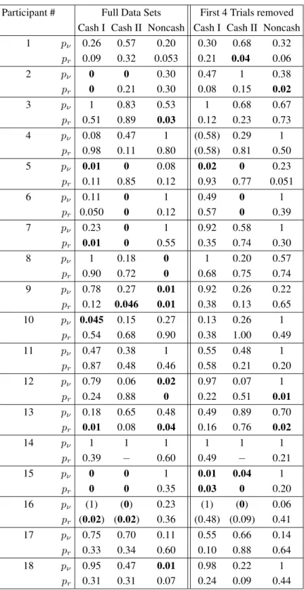
are given in Table 5 under the heading8_{“Full Data Sets”.}

The R code computes simulated random permutations of the data: We used 10,000 such pseudo-random

permuta-tion iterapermuta-tions per analysis. Values ofpνandprsmaller

than 0.05 are marked inbold. Values that would round to

0.05 are given to three significant digits. Cases where the linear order model is rejected are in parentheses. Cases that were undefined due to division by zero are marked

with a−. We confirm Birnbaum’s finding that, in Cash I,

four values ofpνare smaller than0.05.9In addition, there

are six such values in Cash II and four in Noncash. For

pr, Birnbaum (2012) reports six values smaller than0.05

in Cash I, and we find five in each stimulus set. How-ever, it is important to note that not a single individual generated small values ofpνorprfor all three sets.

Following the train of thought in Birnbaum (2012), each of these “significant” values might suggest, by it-self, that the participant might violate iid sampling. How-ever, the Noncash case has relatively few “violations”, even though this should be the prime source of poten-tial memory effects that could cause interdependencies and/or make the probabilities change in some systematic way. This lack of replicability is consistent with our con-cern in the previous section, namely that small values of

pν and/orprmay be difficult to interpret. On the other

hand, if we give MB the benefit of the doubt and we pre-sume that the tests really do detect violations of iid, then the lack of replications could alternatively be interpreted as indicating very small effect sizes. In that case, the iid

7_{See the gamble pairs on Trials 1, 5, 9, etc. versus the gamble pairs}

on Trials 4, 8, 12, etc. in Table 1, keeping in mind that numerical prob-abilities were not provided.

8_{Table 5 shows no major changes with the first 4 trials dropped. We}

provide the rationale for this analysis later.

9_{Birnbaum initially reported a larger number of violations. After the}

Regenwetter lab had difficulties replicating his results, he corrected his data extraction program, and reported (Birnbaum, 2012) values ofpν andprfor Cash I that members of the Regenwetter lab (Y. Cha and M. Choi) were able to confirm independently.

assumption might be violated, but only so slightly that it does not turn up significant very often. In that case, the question would arise how the analysis of RDDS would really be affected by an iid assumption that is only an ap-proximation, but a close apap-proximation, of the data.

We have shown that the RDDS data pass Smith and Batchelder’s (2008) test of iid sampling with top marks.

We have shown that Birnbaum’s (2012) statisticspνand

pr may not be p-values, that their Type-I error rates are

unknown, and that these statistics appear to depend on more than just iid sampling alone, they even appear to depend on how data are coded. We have now established that no single participant, out of 18 participants, has

con-sistently small values of pν and/or pr across all three

stimulus sets, either. Combining these observations, we see no merit in interpreting values ofpν < 0.05and/or pr<0.05as pin-pointing individual participants who

vi-olate iid sampling. Likewise, we see no justification for the much broader blanket statement that “the data of Re-genwetter, et al. (2011) do not satisfy the iid assumptions required by their method of analysis” (Birnbaum, 2012, p. 99).

6 Could RDDS’s findings be an

ar-tifact of warm-up effects?

The discussion around Birnbaum’s (2012) Table 2 sug-gests that decision makers might change their choice probability after the first few trials. We consider whether the great model fit in RDDS could be an accidental ar-tifact of drifting choice probabilities in the first few tri-als due to some sort of warm-up period during which the decision makers familiarized themselves with the experi-ment.

Since Birnbaum (2012) stressed that violations of iid sampling may have led to false acceptance of the linear order model in Regenwetter et al. (2011), we consider whether, by dropping the first four of twenty trials for all gamble pairs, we are able to reject the linear order model on more participants. Starting from Birnbaum’s (2012) Table 2, we dropped the first four trials for each gamble pair, every stimulus set, and every participant. Note that, to decide how many trials to drop, we inspected the data of only the one participant and one stimulus set discussed

in Birnbaum’s (2012) Table 2.10

Table 6 shows the results of two analyses of the data in Regenwetter et al. (2011) using a newer software for

10_{This is important because looking at data to generate a hypothesis}

(11)

Table 5: Summary ofpνandprvalues, rounded to two significant digits, according to the method of Birnbaum (2012)

for Cash I, Cash II, and Noncash of Regenwetter et al. (2011), for both the full data sets, as well as the reduced data sets where the first four trials for each gamble pair pair were dropped.

Participant # Full Data Sets First 4 Trials removed

Cash I Cash II Noncash Cash I Cash II Noncash

1 pν 0.26 0.57 0.20 0.30 0.68 0.32

pr 0.09 0.32 0.053 0.21 0.04 0.06

2 pν 0 0 0.30 0.47 1 0.38

pr 0 0.21 0.30 0.08 0.15 0.02

3 pν 1 0.83 0.53 1 0.68 0.67

pr 0.51 0.89 0.03 0.12 0.23 0.73

4 pν 0.08 0.47 1 (0.58) 0.29 1

pr 0.98 0.11 0.80 (0.58) 0.81 0.50

5 pν 0.01 0 0.08 0.02 0 0.23

pr 0.11 0.85 0.12 0.93 0.77 0.051

6 pν 0.11 0 1 0.49 0 1

pr 0.050 0 0.12 0.57 0 0.39

7 pν 0.23 0 1 0.92 0.58 1

pr 0.01 0 0.55 0.35 0.74 0.30

8 pν 1 0.18 0 1 0.20 0.57

pr 0.90 0.72 0 0.68 0.75 0.74

9 pν 0.78 0.27 0.01 0.92 0.26 0.22

pr 0.12 0.046 0.01 0.38 0.13 0.65

10 pν 0.045 0.15 0.27 0.13 0.26 1 pr 0.54 0.68 0.90 0.38 1.00 0.49

11 pν 0.47 0.38 1 0.55 0.48 1

pr 0.87 0.48 0.46 0.58 0.21 0.20

12 pν 0.79 0.06 0.02 0.97 0.07 1

pr 0.24 0.88 0 0.22 0.51 0.01

13 pν 0.18 0.65 0.48 0.49 0.89 0.70

pr 0.01 0.08 0.04 0.16 0.76 0.02

14 pν 1 1 1 1 1 1

pr 0.39 − 0.60 0.49 − 0.21

15 pν 0 0 1 0.01 0.04 1

pr 0 0 0.35 0.03 0 0.20

16 pν (1) (0) 0.23 (1) (0) 0.06

pr (0.02) (0.02) 0.36 (0.48) (0.09) 0.41

17 pν 0.75 0.70 0.11 0.55 0.66 0.14

pr 0.33 0.34 0.60 0.10 0.88 0.64

18 pν 0.95 0.47 0.01 0.98 0.22 1

(12)

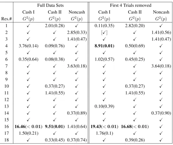
Table 6: Analysis of the linear order model on the full data sets and on reduced data sets where the first four trials for

each gamble pair are dropped. A checkmarkX_{indicates perfect fit.}

Full Data Sets First 4 Trials removed

Cash I Cash II Noncash Cash I Cash II Noncash

Res.# G2₍

p) G2₍

p) G2₍ p)

1 X 2.01(0.28) X 0.11(0.35) 2.82(0.20) X

2 X X _2.85(0.33) _[X_] X _1.41(0.56)

3 X X 1.41(0.47) X X 1.41(0.47)

4 3.76(0.14) 0.09(0.76) X _8.91(0.01) _0.50(0.69) X

5 X X X X X X

6 0.35(0.64) 0.08(0.38) X 1.02(0.57) 0.45(0.25) X

7 X X _3.63(0.18) X X _3.64(0.18)

8 X X X X X X

9 X X X X X X

10 X 0.37(0.27) X X 0.37(0.27) X

11 X _1.41(0.55) X X _1.41(0.55) X

12 X X X X X X

13 X X X _0.10(0.39) X X

14 X X 0.37(0.89) X X 0.37(0.90)

15 X X X X X X

16 16.46(<0_.01₎ _9.51(0.01) _1.41(0.64) _19.43₍_<0_.01₎ _16.68₍_<0_.01₎ X

17 1.50(0.21) X X _1.76(0.1) X X

18 X 0.33(0.45) 0.37(0.74) X 0.39(0.26) X

order-constrained inference.11 _{A checkmark}_X_indicates

perfect fit, where the choice proportions fully satisfy the triangle inequalities, hence the model cannot be rejected

no matter how small the significance levelα. For all cases

with choice proportions outside the linear order model,

we provide the test statisticG2

followed by itsp-value.

G2

values cannot be compared across cells due to order-constrained inference. Significant violations of the linear

order model are marked inbold. One analysis[marked

in brackets]involved prior inspection of the data. As we

drop the first four trials for all stimuli and participants the linear order model fits the data again very well. One person, Participant 16, violates Cash I and Cash II sig-nificantly in the full data sets. This person also violates the model in the reduced data. As we move from the full to the reduced data, one nonsignificant violation becomes significant (Participant 4, Cash I), two nonsignificant vi-olations become perfect fits and two perfect fits become

11_{The new software implemented an improved algorithm for}

order-constrained inference with higher speed and precision. See http://labs.psychology.illinois.edu/labs/DecisionMakingLab/qtest/. As a consequence, the Full Data analysis slightly differs numerically from the results table in Regenwetter et al. (2011).

nonsignificant violations, giving a nearly identical overall picture of goodness-of-fit. This pattern of results demon-strates clearly that the excellent fit of the model in RDDS was not an artifact of a potential 4-trial-per-gamble-pair warm-up as Birnbaum’s (2012) discussion of his Figure 2 seems to suggest.

7 What do Birnbaum’s (2012)

hy-pothetical data tell us about

“true-and-error” models?

Linear orders are a type of transitive preference.12RDDS

tested the linear order model as a proxy for testing tran-sitivity of preferences when preferences are allowed to vary between and within persons. Birnbaum (2012) pro-vided three tables of hypothetical data to suggest that one can construct thought experiments in which the ap-proach of RDDS will classify all three data sets as transi-tive when Birnbaum generated some of the hypothetical

12_{Transitivity states that if}_A_{is preferred to}_B_and_B_{is preferred to}

(13)

data by simulating certain intransitive decision makers. Birnbaum (2012) suggested that “true-and-error” mod-els overcome this challenge. We will now explain briefly how a “true-and-error” model works and then prove that such models do not overcome the stated challenge.

Consider once again Table 1 with the first 36 trials in the RDDS experiment. The basic unit of analysis in RDDS is the binary response on one trial. In contrast, the basic unit of analysis and the basic theoretical primi-tive in “true-and-error” models is that of a “response pat-tern”. Consider the Cash II gamble set. Because Cash II involved five distinct lotteries and all possible pairs of these five gambles, there are 10 distinct pairs of gam-bles in Cash II, each of which was presented 20 times. Each of Trials 4, 8, 12, 16, 20, 24, 28, and 32 is the “first replicate” of a gamble pair in Cash II, whereas Trial 36 is the “second replicate” of the lottery pair used previ-ously in Trial 4. In a “true-and-error” model, the pattern of responses in Trials 4, 8, 12, 16, 20, 24, 28, 32 (and

two more later trials), namelyRRRLRLRR . . ., form

one observation, namely the observed choice pattern for thefirst replicate(see the underlined responses in the last column of Table 1). The second replicate overlaps with the first in time in that Trial 36 is already part of the

ob-served pattern for the second replicate. We call

block-ing assumption the assumption that pairwise choices in Trials 4, 8, 12, 16, 20, 24, 28, 32, and two more later trials can be blocked together to form a single observa-tionRRRLRLRR . . . of one pattern. According to the blocking assumption, the pairwise choice in Trial 36 is not interchangeable with the choice in Trial 4, because Trial 36 is part of the second “replicate”. In Table 1 the respondent happens to have chosen R again as in Trial 4, but if this observed choice were L, the blocking assump-tion would disallow exchanging the observaassump-tions in Trials 4 and 36.

In the analysis of RDDS, the 200 trials that make up the data for a given stimulus set (say, Cash II) are treated as 20 observations for each of 10 binomials (this gives the usual 20 observations per binomial that is recommended as a rule of thumb for using asymptotic statistics). In a “true and error model” the same 200 binary choices form 20 observations (20 observed patterns from 20 replicates)

of one single multinomial with210 _{= 1}

,024cells, i.e., with 1,023 degrees of freedom. This is because there are 1,024 distinct possible patterns of 10 binary choices. For a multinomial with over 1,000 degrees of freedom, 20

ob-servations can be labeledextremely sparse data that are

nowhere close to warranting the use of asymptotic distri-butions for test statistics.

We now introduce what we will label thestandard

true-and-error model [henceforth STE] for such a multino-mial. The STE model spells out how a binary response pattern, the primitive unit of observation for the model, is

related to individual binary responses on individual trials. In the STE model the decision maker has a single, deter-ministic, fixed, “true” preference pattern throughout the experiment, and the reason that he or she does not choose consistently with that preference pattern is because she or he makes errors (trembles) with some probability. Ac-cording to Birnbaum (2004, pp. 59, 61), Birnbaum (2007, p. 163), Birnbaum and Bahra (2007, p. 1024), Birnbaum and Gutierrez (2007, p. 100), Birnbaum (2008a, p. 483), Birnbaum (2008b, p. 315), Birnbaum and Lacroix (2008, p. 125), Birnbaum and Schmidt (2008, p. 82), Birnbaum (2010, p. 369), as well as Birnbaum and Schmidt (2010, p. 604), errors occur independently of each other, with the error probability of each gamble pair being constant over time. Denoting the decision maker’s true preference

pat-tern asBand lettingBsdenote the entry inBfor gamble

pairs, i.e., the person’s true preference for gamble pair

s, and denoting bypsthe probability of making an error

when responding to gamble pair s, the probability that

this decision maker gives responseXsat timetdoes not

depend ontand it equals

(

(1−ps) ifXs=Bs (no error),

ps ifXs6=Bs (error).

(5)

For example, suppose that there are 10 pairs of gam-bles. Following the equations in the referenced papers, the probability of a binary pattern in which a given deci-sion maker chooses correctly on Gamble Pairs 6, 7, and 10 and chooses incorrectly on Gamble Pairs 1, 2, 3, 4, 5, 8, 9 , according to the STE model, is

p1p2p3p4p5(1−p6)(1−p7)p8p9(1−p10). (6)

There are 1,024 such formulae to provide the probabili-ties of all 1,024 different choice patterns that are possible in the STE model. In Table 1 we used labels L and R to refer to left-hand-side and right-hand-side gambles. In-stead, we could also label one gamble as Gamble 0 and the other gamble as Gamble 1 (and in the process drop the distinction of the side on which a given gamble was presented visually), and then record, for each trial a zero or a one to code which gamble was chosen. If we fix the sequence by which we consider the gamble pairs in

such a binary coding13_{, we can represent both the “true”}

preference and each of the observed preference patterns as 10-digit strings of zeros and ones.

Say, if the decision maker’s true preference is binary

pattern0000000000 then, by Formula 6, the observed

pattern 1111100110 has probability p1p2p3p4p5(1 −

p6)(1−p7)p8p9(1−p10). The STE model also spells

13_{This means we disregard the sequence of trial presentations within}

(14)

out what happens if each question (gamble pair) is pre-sented on two replicates. If the decision maker makes 10 choices on 10 distinct gamble pairs in one replicate, and another set of 10 choices on the same 10 gamble pairs in a second replicate, the probability that s/he makes 10 errors on the first replicate and makes no errors on the second replicate, according to STE is,

10 Y

j=1 pj

| {z }

errors on items 1-10 first replicate

×

10 Y

i=1

(1−pi)

| {z }

correct choices on items 1-10 second replicate

. (7)

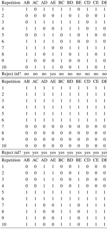
We now move to the hypothetical data in Birnbaum (2012). Birnbaum (2012) argued that the linear order model analysis of RDDS may fail to distinguish transi-tive from intransitransi-tive cases when iid is violated. For con-venience, we reproduce the hypothetical data in question in Table 7. The columns list hypothetical gamble pairs, the rows list the hypothetical replicates (repetitions). In the interior of the table an entry “1” indicates the choice of the first gamble in the gamble pair, and a “0” indicates a choice of the second gamble in a gamble pair.

Our table also gives the results of the iid test of Smith and Batchelder (2008). For the top data set, there are 10 separate tests, of which one turns out significant. Birnbaum (2012) states that these data were iid gen-erated, hence we have one Type I error by Smith and Batchelder’s (2008) test in ten tests. (Recall that our anal-ysis in Table 2 yielded significant results in 3% of cases in RDDS.) In the data in the center of Table 7, all columns are the same, hence we only need to apply Smith and Batchelder’s test once. Indeed, it is significant, consis-tent with a violation of iid sampling. In the third data set, which involves only two types of column collections, the corresponding two tests of Smith and Batchelder (2008) turn out significant both times, consistent with a violation of iid sampling. Birnbaum’s (2012) latter two hypotheti-cal data sets are quite different from RDDS’ real data.

Birnbaum (2012) stated that the RDDS analysis, by counting pairwise choice proportions only, treat the three tables the same and classify all three cases as transitive, whereas true-and error models would distinguish the first, transitive, case from the other two, intransitive, cases. We first show that standard true-and-error models (as used in Birnbaum 2004, pp. 59, 61; Birnbaum, 2007, p. 163; Birnbaum & Bahra, 2007, p. 1024; Birnbaum & Gutier-rez, 2007, p. 100; Birnbaum, 2008a, p. 483; Birnbaum, 2008b, p. 315; Birnbaum and Lacroix, 2008, p. 125; Birn-baum & Schmidt, 2008, p. 82; BirnBirn-baum, 2010, p. 369; Birnbaum & Schmidt, 2010, p. 604), will also treat all three tables the same and will likewise classify all three data tables as transitive. For each of Tables A.4-A.6 in Birnbaum (2012), we can expand the formulations of the

STE model in Formulae 5 and 7 to a situation with 10 replicates. The probability of the observations in each ta-ble is given by

10 Y

i=1

[Bi(1−pi) + (1−Bi)pi] 6

| {z }

each column ofM

contains 6 ones

×

10 Y

j=1

[Bjpj+ (1−Bj)(1−pj)] 4

| {z }

each column ofM

contains 4 zeros

. (8)

For example, if the true preference isB = 1111111111,

the probability of the data in each table is given by

10 Y

i=1

[(1−pi)] 6

| {z }

each column ofM

contains 6 correct choices ×

10 Y

j=1

[pj] 4

| {z }

each column ofM

contains 4 errors

. (9)

If, as is usually the case, we restrict the error probabilities to beps < 0.5,∀s, then the maximum likelihood

esti-mate will yield the “true” preference pattern 1111111111

and estimated error probabilities of0.4 for every error

term, in every one of the three Tables A.4-A.6 of Birn-baum (2012), as summarized in our Table 7. The STE model analysis cannot distinguish the three hypothetical data tables. Birnbaum (2012) designed these three hypo-thetical data sets to illustrate alleged weaknesses of the analysis of RDDS and strengths of the “true-and-error” approach. Yet, like the analysis used in RDDS, the STE model analysis cannot differentiate between the data in the three tables either, and it will also classify all three cases as transitive.

In the discussion of Tables A.4-A.6, Birnbaum (2012,

p. 106) states that Birnbaum and Bahra (2007) “found

that some people had 20 responses out of 20 choice prob-lems exactly the opposite between two blocks of trials. Such extreme cases of perfect reversal mean that iid is not tenable because they are so improbable given the

as-sumption of iid.” If true, then this would mean that

Birn-baum and Bahra’s (2007) analysis, which used a STE model with iid errors (Birnbaum and Bahra, 2007, p. 1024), is itself “not tenable” on those data, in Birnbaum’s words.

(15)

Table 7: Hypothetical data in Birnbaum’s (2012) Tables A.4 (top), A.5. (center), and A.6. (bottom). A “1” indicates choice of the first option in pair, a “0” indicates choice of the second option. For each column of data, we also provide the result of a test for iid sampling of Smith and Batchelder (2008, p.727) using confidence intervals of point estimates

±2 standard errors (or±1.96 standard errors. The results of using 1.96 or 2 standard errors matched throughout.).

Repetition AB AC AD AE BC BD BE CD CE DE

1 1 0 1 1 1 1 0 1 1 1

2 0 0 0 0 1 0 1 0 0 1

3 0 1 1 1 1 1 1 0 1 1

4 1 1 0 0 1 1 1 0 1 0

5 0 0 1 1 0 1 0 1 0 0

6 1 1 1 1 0 1 0 0 1 0

7 1 1 1 0 0 1 1 1 1 1

8 1 1 0 1 1 0 1 1 0 1

9 1 0 0 0 1 0 0 1 1 0

10 0 1 1 1 0 0 1 1 0 1

Reject iid? no no no yes no no no no no no

1 1 1 1 1 1 1 1 1 1 1

2 1 1 1 1 1 1 1 1 1 1

3 1 1 1 1 1 1 1 1 1 1

4 1 1 1 1 1 1 1 1 1 1

5 1 1 1 1 1 1 1 1 1 1

6 1 1 1 1 1 1 1 1 1 1

7 0 0 0 0 0 0 0 0 0 0

8 0 0 0 0 0 0 0 0 0 0

9 0 0 0 0 0 0 0 0 0 0

10 0 0 0 0 0 0 0 0 0 0

Reject iid? yes yes yes yes yes yes yes yes yes yes

1 0 0 1 1 0 0 1 0 0 0

2 0 0 1 1 0 0 1 0 0 0

3 0 0 1 1 0 0 1 0 0 0

4 0 0 1 1 0 0 1 0 0 0

5 1 1 1 1 1 1 1 1 1 1

6 1 1 1 1 1 1 1 1 1 1

7 1 1 0 0 1 1 0 1 1 1

8 1 1 0 0 1 1 0 1 1 1

9 1 1 0 0 1 1 0 1 1 1

10 1 1 0 0 1 1 0 1 1 1

Reject iid? yes yes yes yes yes yes yes yes yes yes

Next, consider a modification of the STE model test in which there is still a single true preference, but where

(16)

can originate from a person with transitive true prefer-ence pattern 1111111111 who makes no errors for the first 60 binary choice trials (i.e., the first 6 lines in the table) and who makes errors for all remaining trials of the study. However, this person can instead have fixed intransitive true preference pattern 0011001000 and gen-erate the same data because she or he makes no errors on

the first 6 trials of stimuliAD, AE, BEbut errors in all

first 6 trials of stimuliAB, AC, BC, BD, CD, CE, DE,

then switches to the opposite error behavior for the re-maining four replicates. Similar constructions are possi-ble for Birnbaum’s (2012) Tapossi-bles A.4 and A.6 (top and bottom of our Table 7). If errors are allowed to be inter-dependent and if error probabilities are allowed to change over the course of the experiment, then “true-and-error”

models can generate a perfect fit toanydata, no matter

what fixed “true preference” they use. In other words, “true-and-error” models without iid assumption for errors are neither identifiable nor testable. They are vacuous, even if they permit only one single and fixed “true” pref-erence.

Finally, we consider what happens in Tables A.4-A.6 (our Table 7) if we consider “true-and-error” models in which the preferences are allowed to vary. For example,

a person may have preference patternB1 = 1111111111,

say, 60% of the time, and preference pattern B0 =

0000000000on 40% of occasions. We denote this as Hypothesis H. Or the person may have preference state

B2 = 0011001000, say, 60% of the time, and B3 = 1100110111the other 40% of the time. We denote this as Hypothesis HH.

WriteXt

sfor the decision maker’s observed choice for

gamble pairsat replicatet, that is,Xt

sis the entry in a

given table in columns and rowt. Assume for a

mo-ment, that there are no errors, i.e., ps = 0, for s ∈

{AB, AC, AD, AE, BC, BD, BE, CD, CE, DE}. We obtain a perfect fit for the data in each of Tables A.4– A.6 in Birnbaum (2012) under Hypothesis H by

assum-ing that the decision maker is in stateB1whenever he

or she gives an answerXt

s= 1in the Table, and that the

decision maker is in stateB0whenever he or she gives an

answerXt

s = 0in the Table. Likewise, we obtain a

per-fect fit of the data in each of Tables A.4-A.6 in Birnbaum (2012) by assuming that the decision maker is in state

         

        

B2 ifXt

s= 0, and

s∈ {AB, AC, BC, BD, CD, CE, DE}, B2 ifXt

s= 1, ands∈ {AD, AE, BE}, B3 ifXt

s= 1, and

s∈ {AB, AC, BC, BD, CD, CE, DE}, B3 ifXt

s= 0, ands∈ {AD, AE, BE}.

In a “true-and-error”model test where preference patterns may vary at any time, both Hypothesis H and

Hypothe-sis HH will fit the data in all three tables perfectly even when setting all error probabilities to zero. The “true-and-error” model with variable preferences is

unidentifi-able and can generate a perfect fit toanydata whatsoever,

such as those in Tables A.4-A.6 in Birnbaum (2012). Like the previous case, this “true-and-error” model is vacuous. Combining the last two points, if “true preferences” can vary at any time, if the error probabilities are posi-tive, if these error probabilities are allowed to change at any time, and if errors are allowed to be interdependent, the unidentifiability and nontestability problem is further exacerbated and multiple mutually exclusive

“true-and-error” models will vacuously and simultaneously fitany

data perfectly.

How does MB propose to render tests of “true-and-error” models vacuous? First, accommodating

non-iid errors seems challenging.14 _{Second, MB uses a}

“blocking” assumption, not needed by RDDS, which reg-ulates, at the researcher’s discretion, when exactly pref-erences are permitted to change. Under the “blocking” assumption, preferences are fixed during replicates and preferences are permitted to change from one replicate to the next. In other words, the decision maker must keep or may change their preference at arbitrarily de-termined time points that are selected by the scholar but not communicated to the participant. Considering Table 1, the blocking assumption for a “true-and-error” model with variable preferences from one block to the next as-sumes that the decision maker stays in the first true pref-erence for the first replicate of those two gamble pairs that were not yet presented in the first 36 trials, whereas the decision maker is allowed to have already moved to a new preference state for the second replicate as of Trial 36 where we observe the second replicate of the

lot-tery pair “36%chance of$24.44” versus “28%chance

of$31.43”. It is the “blocking” assumption that allows

Birnbaum (2012) to gather data into tables like Tables A.4-A.6 where each row is interpreted as one fixed pref-erence state. Our example above has shown that in the absence of the “blocking” assumption both Hypotheses H and HH can simultaneously fit all the data in the three tables perfectly, even though they are mutually incompat-ible, hence the model becomes vacuous and uninforma-tive. The sequence of trials in RDDS in Table 1, where the second replicate starts on Trial 36 (for some gamble pairs) before the first replicate has even been completed (for some other gamble pairs), shows how implausible it is to assume that a decision maker switches preferences between, but not within, blocks of trials that form a repli-cate. The decision maker has no way of knowing when she or he may use the first preference state and when she or he may use the second preference state. Similar

con-14_{Note that, while the analysis in RDDS only uses iid in its test}

(17)

cerns apply also when replicates are fully separated in time and do not overlap.

8 Conclusion.

Every researcher depends on some simplifying assump-tions. The state-of-the-art “order-constrained likelihood-ratio” test in RDDS is currently available only under the auxiliary assumption of iid data. Our application of Smith and Batchelder’s (2008) test suggests that RDDS’ data, indeed, satisfy that iid assumption. Birnbaum’s (2012) inference that the RDDS data violate iid rests on ques-tionable mathematical conjectures and leads to incoher-ent interpretations within participants. In particular, Birn-baum’s proposed test statistics have unknown Type-I er-ror rates that are sometimes larger, sometimes smaller

than the nominalα-level, even for the same data,

depend-ing on how responses are coded.

Reducing 200 observations for a given stimulus set to a manageable set of statistics that can serve as point es-timates of parameters and ultimately help test theories, requires making one assumption or another. We have shown that Birnbaum’s proposed alternative rests on its own, highly restrictive assumptions, some of which, to date, have not been tested. Not only are the errors rou-tinely assumed to be iid, the analysis also fundamen-tally depends on the “blocking” assumptions according to which pairwise choices at certain time points, such as Trials 4, 8, 12, 16, 20, 24, 28, 32, and two more trials af-ter Trial 36 in RDDS (see Table 1) form one observation, whereas another collection of trials (starting with Trial 36 in Table 1) form another observation. Using Birnbaum’s (2012) hypothetical data, we have illustrated how drop-ping these assumptions would make the “true-and-error” models vacuous and uninformative. A companion paper has shown that, while many classical probabilistic choice models, such as Luce’s (1959) choice model, the weak utility model (Becker et al.,1963; Block & Marschak, 1960; Luce & Suppes, 1965; Marschak, 1960), and the most heavily used “true-and-error” model in the litera-ture (Birnbaum (2004, 2007, 2008a,b, 2010; Birnbaum & Bahra, 2007; Birnbaum & Gutierrez, 2007; Birnbaum & Lacroix, 2008; Birnbaum & Schmidt, 2008, 2010), re-quire a person to have a single fixed preference through-out an entire experiment, the model in RDDS not only al-lows preferences to be probabilistic, it even has the some-what unique property that one can average different prob-ability distributions satisfying the model, and still satisfy the model. Not only does the model in RDDS stand out in its ability to model variability of preferences, it even allows that variability itself to be non-stationary.

We have shown that MB’s inference of iid violations in the RDDS data are premature: The RDDS data do not

ap-pear to violate iid sampling. We have also provided some documentation on Birnbaum’s own (2012) hypothetical data, suggesting the opposite of Birnbaum’s (2012) con-clusion: “True-and-error” models hinge far more strongly on their assumptions than does the analysis in RDDS.

References

Becker, G. M., DeGroot, M. H., & Marschak, J. (1963).

Stochastic models of choice behavior.Behavioral

Sci-ence, 8, 41–55.

Birnbaum, M. (2004). Tests of rank-dependent utility and cumulative prospect theory in gambles represented by natural frequencies: Effects of format, event framing,

and branch splitting.Organizational Behavior and

Hu-man Decision Processes, 95, 40–65.

Birnbaum, M. (2007). Tests of branch splitting and

branch-splitting independence in Allais paradoxes with

positive and mixed consequences.Organizational

Be-havior and Human Decision Processes, 102, 154–173.

Birnbaum, M. (2008a). New paradoxes in risky decision

making.Psychological Review, 115, 463–501.

Birnbaum, M. (2008b). New tests of cumulative prospect theory and the priority heuristic: Probability-outcome

tradeoff with branch splitting.Judgment and Decision

Making, 3, 304–316.

Birnbaum, M. (2010). Testing lexicographic semiorders as models of decision making: Priority dominance,