ATLAS measurements of the properties of jets for boosted particle searches
G. Aadet al.*(ATLAS Collaboration)
(Received 23 June 2012; published 15 October 2012)
Measurements are presented of the properties of high transverse momentum jets, produced in proton-proton collisions at a center-of-mass energy of pffiffiffis
¼7 TeV. The data correspond to an integrated luminosity of35 pb1and were collected with the ATLAS detector in 2010. Jet mass, width, eccentricity,
planar flow and angularity are measured for jets reconstructed using the anti-kt algorithm with distance parametersR¼0:6and 1.0, with transverse momentumpT>300 GeVand pseudorapidityjj<2. The measurements are compared to the expectations of Monte Carlo generators that match leading-logarithmic parton showers to leading-order, or next-to-leading-order, matrix elements. The generators describe the general features of the jets, although discrepancies are observed in some distributions.
DOI:10.1103/PhysRevD.86.072006 PACS numbers: 12.38.t, 13.30.Eg
I. INTRODUCTION
The high center-of-mass energy at the Large Hadron Collider (LHC) combined with the coverage and gran-ularity of the ATLAS calorimeter provide an excellent environment to study hadronic jets. Measurements of dijet cross sections [1,2], jet shapes [3,4], jet substruc-ture [5] and angular correlations [6,7] have already been published using the data taken by the ATLAS and CMS Collaborations in 2010.
Massive, hadronically decaying particles produced with a significant boost (such as top quarks, Higgs bosons, or new particles) will tend to have collimated decays, such that their decay products are contained within a single jet. The substructure of jets resulting from such decays is expected to result in deviations in the observables mea-sured here for light quarks and gluons, thus providing discriminating power in heavy particle searches.
The observable jet properties presented here are mass, width, eccentricity, planar flow and angularity. All of these have been shown to be useful in Monte Carlo studies in the search for high transverse momentum (pT), massive parti-cles [8–14], and together they provide an important set of probes of the substructure of jets.
Three of these (mass, planar flow and angularity) have recently been measured by CDF [13] at the Tevatron. Angularities are a family of infrared-safe quantities that have characteristic distributions for two-body decays, while planar flow discriminates between two-body and many-body decays and, for large jet masses (above about 100 GeV), is largely independent of the jet mass. Eccentricity is a complementary observable to planar flow, with which it is highly anticorrelated. Jet width is a
dimensionless quantity related to the jet mass and is thus expected to retain much of the discriminatory power with-out being as sensitive to the detector effects on energy scale and resolution that can hinder a mass measurement.
Jet substructure measurements can be particularly vul-nerable to ‘‘pileup,’’ i.e. particles produced in multiplepp
interactions that occur in addition to the primary interac-tion, within the sensitive time of the detector. These addi-tional interactions result in diffuse, usually soft, energy deposits throughout the central region of the detector—the region of interest for the study of high-pT jets. This addi-tional energy deposition can be characterized by the num-ber of reconstructed primary vertices (NPV) [15,16], with events having a single good vertex (NPV¼1) being con-sidered free from the effects of pileup. The 2010 ATLAS data set provides a unique opportunity to study these effects; a significant fraction of the 2010 data set comprises
NPV¼1events, making this data set ideal for evaluating the effects of pileup on jet substructure measurements. This data set has an averageNPV’2:2.
II. THE ATLAS DETECTOR
The ATLAS detector [17] at the LHC was designed to study a wide range of physics. It covers almost the entire solid angle around the collision point with layers of track-ing detectors, calorimeters and muon chambers. Tracks and vertices are reconstructed with the inner detector, which consists of a silicon pixel detector, a silicon strip detector and a transition radiation tracker, all immersed in a 2 T axial magnetic field provided by a superconducting solenoid.
The ATLAS reference system is a Cartesian right-handed coordinate system, with the nominal collision point at the origin. The anticlockwise beam direction defines the positive z axis, while the positive x axis is defined as pointing from the collision point to the center of the LHC ring and the positive y axis points upwards. The azimuthal angle is measured around the beam axis,
*Full author list given at the end of the article.
Published by the American Physical Society under the terms of the Creative Commons Attribution 3.0 License. Further distri-bution of this work must maintain attridistri-bution to the author(s) and the published article’s title, journal citation, and DOI.
and the polar angleis the angle measured with respect to the z axis. The pseudorapidity is given by ¼ ln tanð=2Þ. Transverse momentum is defined relative to the beam axis.
For the measurements presented here, the high-granularity calorimeter systems are of particular impor-tance. The ATLAS calorimeter system provides fine-grained measurements of shower energy depositions over a large range in.
Electromagnetic calorimetry in the range jj<4:9 is provided by liquid-argon (LAr) sampling calorimeters. This calorimeter system enables measurements of the shower energy in up to four depth segments. For the jets measured here, the transverse granularity ranges from
0:0030:10to 0:100:10in , depending on depth segment and pseudorapidity.
Hadronic calorimetry in the rangejj<1:7is provided by a steel/scintillator-tile sampling calorimeter. This sys-tem enables measurements of the shower energy deposition in three depth segments at a transverse granularity of typically 0:10:1. In the end caps (jj>1:5), LAr technology is used for the hadronic calorimeters that match the outer limits of the electromagnetic end-cap calorimeters. This system enables four measurements in depth of the shower energy deposition at a transverse granularity of either0:10:1(1:5<jj<2:5) or0:2 0:2(2:5<jj<3:2).
III. MONTE CARLO SIMULATION
The QCD predictions for the hadronic final state in inelasticpp collisions are based on several Monte Carlo generators with different tunes.
The PYTHIA 6.423 generator [18] with the ATLAS Minimum Bias Tune 1 (AMBT1) [19] parameter set is used as the primary generator for comparisons with the data and for extracting corrections to the data for detector effects. TheAMBT1tune uses the MRSTLO [20] parton distribu-tion funcdistribu-tion (PDF) set with leading-order (LO) perturba-tive QCD matrix elements for 2!2 processes and a leading-logarithmic, pT-ordered parton shower followed by fragmentation into final-state particles using a string model [21] with Lund functions [22] for light quarks and Bowler functions [23] for heavy quarks. In addition to charged particle measurements from ATLAS minimum bias data [24,25], the AMBT1 tune uses data from LEP, SPS and the Tevatron.
An additionalPYTHIAtune,PERUGIA2010[26,27], is used for comparison with AMBT1. The PERUGIA2010 tune also uses data from LEP, SPS and the Tevatron and additionally improves the description of jet shape measurements in LEP data. The CTEQ5L [28] PDF set is used. This tune of PYTHIAis used in the calculation of the systematic uncer-tainties on the measurements and for comparison with the data, along with the HERWIG++ 2.4.2 generator with its default settings [29].
The more recentHERWIG++2.5.1 generator is included for comparison with the final measurements at particle level, as are theAUET2Btune [30,31] ofPYTHIA6.423, the POWHEG generator interfaced to this same PYTHIA tune, and the PYTHIA 8.153 generator [32] with tune 4C [27,30]. The major difference between HERWIG++ versions 2.4.2 and 2.5.1 is the inclusion of color reconnections in the latter. ThePOWHEGgenerator, which implements next-to-leading-order (NLO) calculations within a shower Monte Carlo context [33–36], uses the CTEQ6M [28] PDF set.
Generated events are passed through the ATLAS detec-tor simulation program [37], which is based on GEANT4 [38]. The quark-gluon string model with an additional precompound [39] is used for the fragmentation of nuclei, and the Bertini cascade model [40] is used to describe the interactions of hadrons with the nuclear medium.
Monte Carlo events are reconstructed and analyzed using the same event selection and simulated trigger as for the data. The size and position of the collision beam spot and the detailed description of detector conditions during the data-taking runs are included in the simulation.
IV. EVENT SELECTION
Events containing pileup can be identified by the pres-ence of more than one primary vertex in the event, herein referred to as NPV>1. Events recorded in the 2010 ATLAS data set contain an averageNPV’2:2and include a significant fraction of NPV¼1 events (’28%); these may be used for testing the pileup correction methods.
After applying data-quality requirements, the data sam-ple corresponds to a total integrated luminosity of35:0 1:1 pb1 [41,42].
A. Trigger selection
Events must pass the ATLAS first-level trigger requiring a jet (built from calorimeter towers with a granularity of
0:10:1 in ) with transverse energy ET 95 GeV. The selection efficiency of this trigger has been found to be close to 100% for events satisfying the offline selection criteria implemented here, with a negligible de-pendence on jet mass [5].
B. Primary vertex selection
All events are required to have at least one good primary vertex. This is defined as a vertex with at least five tracks withpT>150 MeVand both transverse and longitudinal impact parameters consistent with the LHC beamspot [15,16]. The analysis presented here makes use of the full 2010 data set. The requirement ofNPV¼1is applied only where derivation of pileup corrections is not possible.
C. High-pT jet selection
Jets are reconstructed from locally calibrated topologi-cal clusters [43] using the anti-kt algorithm [44] with
distance parameters of R¼0:6 and 1.0. Jets satisfying
pT>300 GeV and jj<2 are selected for analysis. Any event containing an R¼0:6 jet with pT>30 GeV that fails to satisfy the criteria [45] designed to safeguard against jets caused by transient detector effects and beam backgrounds is excluded from this analysis.
In simulated data, jets are reconstructed from locally calibrated topological clusters to derive corrections for pileup and determine the systematic uncertainties and de-tector correction factors. The corrected data distributions are then compared to Monte Carlo predictions at particle level; in this case jets are reconstructed from stable particles as opposed to clusters. Particles are deemed to be stable for the purpose of jet reconstruction if their mean lifetimes are longer than 10 ps. Neutrinos and muons are excluded, just as they are for the Monte Carlo-based jet energy scale calibration that is applied to the data. This exclusion has a negligible effect on the final measurements.
The total numbers of jets in data satisfying the selection criteria detailed here are 122 000 R¼1:0 jets and
87 000 R¼0:6 jets; however, only the highest pT jet in each event is selected for this analysis. The total num-bers selected for analysis are 83 000 R¼1:0 jets and
62 000R¼0:6jets.
V. SUBSTRUCTURE OBSERVABLES AND THEIR CORRELATIONS
A. Jet mass
The jet mass M is calculated from the energies and momenta of its constituents (particles or clusters) as follows:
M2 ¼X
i Ei 2 X i ~ pi 2 ; (1)
whereEiandp~iare the energy and three-momentum of the
ith constituent. The sum is over all jet constituents in this and all subsequent summations. The standard ATLAS re-construction procedure is followed: clusters have their masses set to zero, while Monte Carlo particles are assigned their correct masses.
B. Jet width
The jet widthW is defined as:
W ¼
P
i Ripi
T P i pi T ; (2)
where Ri¼ ffiffiffiffiffiffiffiffiffiffiffiffiffiffiffiffiffiffiffiffiffiffiffiffiffiffiffiffiffiffiffiffiffiffiffi
ðiÞ2þ ðiÞ2
p
is the radial distance between the jet axis and the ith jet constituent andpi
T is the constituentpTwith respect to the beam axis.
C. Eccentricity
The jet eccentricity E is calculated using a principal
component analysis (PCA) [12]. The PCA method
provides the vector which best describes the energy-weighted geometrical distribution of the jet constituents in theð; Þplane. The eccentricity is used to characterize the deviation of the jet profile from a perfect circle in this plane, and is defined as
E ¼1vmin
vmax; (3)
where vmaxðvminÞ is the maximum (minimum) value of variance of the jet constituents’ positions with respect to the principal vector. The calculation consists of the follow-ing steps:
(1) For each jet the energy-weighted centers inand
are calculated as
jet¼
P
i iEi
P
i Ei
; jet¼ P
i iEi
P
i Ei
; (4)
where the energy and position in theð; Þplane of the ith constituent with respect to the jet axis are denoted byEi,iandi.
(2) The PCA is performed to determine the vector ~x1in
ð; Þ space that passes through the energy-weighted center of the face of the jet and results in a minimum in the variance of the constituents’ positions. The angle of this vector with respect to the jet centerðjet;jetÞis given by
tan2¼
2P
i
Eiii
P
i
Eið2
i2iÞ
(5)
and the angle of the orthogonal vector ~x2is2. (3) The energy-weighted variancesv1 andv2 with
re-spect to ~x1and ~x2 are calculated as
v1¼
1 N
X
i
EiðcosisiniÞ2;
v2 ¼
1 N
X
i
EiðsiniþcosiÞ2; (6)
whereN is the number of constituents.
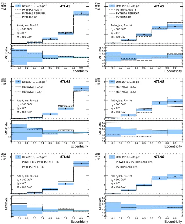
(4) Finally, the largest value of the variance is assigned tovmaxand the smallest tovmin. The jet eccentricity ranges from zero for perfectly circular jets to one for jets that appear pencil-like in theð; Þplane. Eccentricity is measured for jets in the mass rangeM > 100 GeV; this is the mass region of interest for the search for a Higgs boson or other massive, hadronically decaying particles predicted in various extensions to the Standard Model.
D. Planar flow
A variable complementary to the eccentricity is planar flowP[10,46,47]. The planar flow measures the degree to
which the jet’s energy is evenly spread over the plane across the face of the jet (high planar flow) versus spread linearly across the face of the jet (small planar flow).
To calculate planar flow, one first constructs a two-dimensional matrixIkl
E: Ikl E ¼ 1 M X i 1 Ei
pi;kpi;l: (7)
Here, M is the jet mass, Ei is the energy of the ith constituent of the jet and pi;k and pi;l are the k and l components of its transverse momentum calculated with respect to the jet axis. The planar flow is
P¼4detðIEÞ
TrðIEÞ2: (8)
Vanishing or low planar flow corresponds to a linear energy deposition, as in the case of a two-pronged decay, while completely isotropic energy distributions are charac-terized by unit planar flow [10]. Jets with many-body kine-matics are expected to have a planar flow distribution that peaks towards unity. In general, QCD jets have a risingP
distribution that peaks at P¼1; the hadronization process has contributions from many soft gluons and is largely isotropic. However, jets with high pT and high mass are well described by a single hard gluon emission. Consequently, these jets have a planar flow distribution that peaks at a low value [13]. The planar flow distributions are measured in the context of boosted, massive particle searches by applying a mass cut, 130< M <210 GeV, consistent with the window in which one would expect to observe a boosted top quark decay collimated within a single jet. The contribution from top quark decays in this subset of the data is negligible—here we measure the properties of light-quark and gluon jets that constitute a substantial frac-tion of the background in boosted top quark measurements.
E. Angularity
Angularities (a) are a family of observables that are sensitive to the degree of symmetry in the energy flow inside a jet. The general formula for angularity [10] is given by a ¼ 1 M X i
Eisinai½1cosi1a: (9)
Hereais a parameter that can be chosen to emphasize radiation near the edges (a <0) or core (a >0) of the jet,
Mis the jet mass,Eiis the energy of theith jet constituent andiis its angle with respect to the jet axis. In the limit of small-angle radiation (i1),ais approximated by
a’ 2ða1Þ
M
X
i
Eiði2aÞ: (10)
Angularities are infrared-safe for a 2 [13]. In the analysis presented here, Eq. (9) with a value ofa¼ 2
is used. The2observable can be used as a discriminator
for distinguishing QCD jets from boosted particle decays by virtue of the broader tail expected in the QCD distribu-tion [10]. At a given high mass, the angularity of jets with two-body kinematics should peak around a minimum value
peaka ’ ð2Mp TÞ
1a, which corresponds to the two hard
con-stituents being in a symmetric pT configuration around the jet axis. An estimate for the maximum of the distribu-tion can also be calculated in the limit of small-angle radiation, max
a ’ ð2RÞað2MpTÞ [13], which corresponds to a
hard constituent close to the jet axis and a soft constituent on the jet edge.
The measurement of 2 is aimed primarily at testing QCD, which makes predictions for the shape of the 2 distribution in jets where the small-angle approximation is valid. For this reason, this measurement is made only for anti-ktjets withR¼0:6.
Here,2 is measured for jets in the mass range100< M <130 GeV. This mass region is chosen to have mini-mal contributions from hadronically decaying W or Z
bosons or boosted top quarks (PYTHIApredictions estimate a relative fraction below 0.2%).
F. Correlations between the observables The levels of correlation between the variables presented here provide information that is valuable in deciding which variables may potentially be used together in a search for boosted particles. Here the correlation factors between pairs of variables are calculated as their covariance divided by the product of their standard deviations:
¼covðx; yÞ xy
: (11)
Summaries of the correlations between all of the observ-ables studied here are shown in Fig.1forR¼1:0jets in PYTHIA at particle level. The coefficients are shown both with and without a jet mass cut of M >100 GeV—the individual mass constraints for each observable are dropped here to allow the correlations between them to be calculated. Jets subjected to a mass cut are also re-stricted to jj<0:7. This additional restriction on is applied wherever a mass cut is made on the observables presented here; this has a negligible effect on the shapes of the distributions while allowing direct comparisons with other measurements of the same quantities [13].
The strongest correlations observed are those between jet mass and width (85%) and between planar flow and eccentricity (80%). The correlation between mass and width reduces considerably when jets are required to be in the kinematic regionM >100 GeV. This trend is followed by almost all observables. The planar flow and eccentricity, however, are even more strongly anticorrelated in high-mass jets (90%). The correlation between mass andpTis weak (12%–16%). Angularity is largely uncorre-lated with all of the other observables.
VI. CORRECTIONS FOR PILEUP AND DETECTOR EFFECTS
The contribution from pileup is measured using the complementary cone method first introduced by the CDF experiment [13,48]. A complementary cone is drawn at a right angle in azimuth to the jet (comp ¼jet2,
comp¼jet) and the energy deposits in this cone are added into the jet such that the effect on each of the jet properties can be quantified. The shift in each observable after this addition is attributed to pileup and the underlying event (UE), the latter being the diffuse radiation present in all events and partially coherent with the hard scatter. The effects of these two sources are separated by comparing events withNPV¼1(UE only) to those withNPV>1(UE
and pileup): the difference between the average shift for single-vertex and multiple-vertex events is attributed to the contribution from pileup only.
The presence of additional energy in events withNPV>1 affects the substructure observables in different ways; the effect of pileup on the shape of the 2 distribution is negligible (below 1%) in this data set, and so no correc-tions are applied. The other observables under study have their distributions noticeably distorted by the presence of pileup. The pT-dependent corrections for this effect are applied to the mass, width and eccentricity distributions, while the planar flow distribution of high-mass jets is measured only in events withNPV¼1. There are a small number of jets (100anti-kt R¼0:6 jets) in the high-mass range (M >130 GeV), making it too difficult to derive robust pileup corrections for planar flow (which is limited to this mass range in this analysis) in this data set.
A. Pileup corrections forR¼ 0:6jets
The mass shift due to the UE and pileup inNPV¼1and
NPV>1events is shown in Fig.2forR¼0:6jets in the range 300< pT<400 GeV. The shift follows the ex-pected behavior, given by
M¼p0
Mþ
p1M
M ; (12)
where piM and their associated uncertainties are deter-mined from the data. M is the increase in the jet mass due to the addition of the energy deposits in the comple-mentary cone to the jet. Corrections to the jet mass are limited to the region M >30 GeV, as thep1M
M parametri-zation uses a leading-order approximation [48] and is only valid forMM. This has a negligible effect on the final measurements in the rangeM >20 GeV, as illustrated for
FIG. 1 (color online). The correlation coefficients between pairs of variables calculated in PYTHIA at particle level for
R¼1:0 jets with no mass constraint (top panel) and with a mass constraint ofM >100 GeV(bottom panel).
FIG. 2 (color online). The size of the mass shift in anti-kt
R¼0:6jets with300< pT<400 GeVin jets with pileup and UE (NPV>1, averageNPV’2:2) and with UE alone (NPV¼1). The curves are fits of the formM¼p0Mþ
p1M
M . The difference between the curves gives the contribution to the jet mass from pileup only. The 1uncertainties on the fits are shown in the error bands.
R¼1:0jets in Fig.3; low mass, high-pTjets tend to have a small contribution from pileup.
The corresponding parametrizations for the shifts in widthW and eccentricityEare
W¼p0Wþp1WW; E¼p0Eþp1EEþp2EE2: (13)
The pileup corrections for width and eccentricity are applied to jets across the full mass range.
B. Pileup corrections forR ¼ 1:0jets
The complementary cone technique cannot be applied directly to R¼1:0 jets due to the high probability of overlap between the complementary cone and the jet; scaling factors are therefore applied to the corrections measured forR¼0:6jets.
The scaling behavior is determined experimentally by comparing the pileup dependence inR¼0:6andR¼0:4
jets. For each observable, the shifts forR¼0:4jets are fit to a functional form. The shifts forR¼0:6jets are then fit to a scaled version of this function, where all parameters are fixed at theirR¼0:4values and the scaling is the only free parameter of the fit. The measured R dependence is then validated with a comparison betweenR¼1:0jets in
NPV>1andNPV¼1events.
The predicted (observed) behaviors for the scaling of the shifts in mass and width are
M:piMR
4ðR3:5Þ; (14)
W: p0WR
3
ðR2:5
Þ; p1W R
2
ðR1
Þ: (15)
The phenomenological predictions [49] for scaling are used, and the discrepancies between predictions and ob-servations are considered systematic uncertainties in this procedure.
There is no phenomenological prediction for the scaling of E with pileup; therefore the nominal value of the
scaling of the shift in this variable is measured in data. The measurements find the scaling of the parametrization to be a function of mass:
EðM <40 GeVÞ:pi
ER
2;
EðM40 GeVÞ: pi
E R
3: (16)
The measured scaling is varied between R2 and R3 across the mass range in order to determine a conservative estimate of the systematic uncertainty introduced by this procedure.
The performance of the pileup correction procedure in the case of mass, width and eccentricity is shown in Fig.3. The observable most sensitive to pileup is the jet mass; the mean R¼1:0jet mass is shifted upwards by7 GeVin events with NPV>1, and there is a significant change in the shape of the mass distribution. In the case of jet width and eccentricity, the effect of pileup is a small (5%) shift towards wider, less eccentric jets. This supports the expected behavior: width is less sensitive to pileup than mass, making it a promising alternative to mass as a criterion for selecting jets of interest in boosted particle searches in the high pileup conditions of later LHC opera-tions. For all observables the discrepancies between the pileup-corrected distributions and those for events with
NPV¼1are small, and agreement is obtained within the systematic uncertainties on the corrections.
FIG. 3 (color online). The mass, width and eccentricity distri-butions before and after the pileup corrections. The (red) squares indicate the uncorrected data in the full data set, the (black) circles indicate the subset of this data with NPV¼1 and the
(blue) triangles indicate the full data set after pileup corrections. The mean value of each distribution is indicated in the legend with the corresponding statistical uncertainty. The lower region of each figure shows the measured ratio ofNPV>1toNPV¼1
C. Corrections for detector effects
After correcting the distributions for pileup, each distribution is corrected to particle level, using bin-by-bin corrections for detector effects. The bin migrations due to detector effects are determined and controlled by increasing the bin sizes until all bins have a
purity and efficiency above 50% according to Monte Carlo predictions, where purity and efficiency are defined as
pi¼A
partþdet
i
Adet
i
; ei¼A
partþdet
i
Aparti : (17)
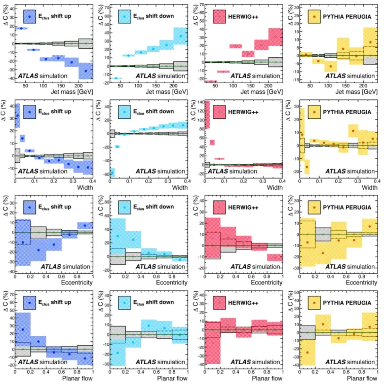
FIG. 4 (color online). The dominant sources of systematic uncertainty on the measurements are those resulting in large variations in the detector correction factorsC. These correction factors are found bin by bin usingR¼0:6jets in aPYTHIA AMBT1sample with upward and downward variations of the cluster energy scale (first and second columns), and by usingHERWIG++(third column) and
PYTHIA PERUGIA2010(fourth column) in place ofPYTHIA AMBT1. The differencesCfound when comparing the correction factors obtained with the baselinePYTHIA AMBT1sample are shown here for each of the properties measured inR¼0:6jets. The shaded bands indicate the statistical uncertainties.
HereAparti þdet is the number of detector-level jets
(re-constructed from locally calibrated clusters) in bini that have a particle-level jet (reconstructed from stable Monte Carlo particles), matched within R <0:2 and falling in the same bin. Aparti is the total number of
particle-level jets in biniandAdet
i is the total number of detector-level jets in bini.
The particle-level value for an observable in bin i is found by multiplying its measured value by the relevant correction factorCi:
FIG. 5 (color online). The dominant sources of systematic uncertainty on the measurements are those resulting in large variations in the detector correction factorsC. These correction factors are found bin by bin usingR¼1:0jets in aPYTHIA AMBT1sample with upward and downward variations of the cluster energy scale (first and second columns), and by usingHERWIG++(third column) and
PYTHIA PERUGIA2010(fourth column) in place ofPYTHIA AMBT1. The differencesCfound when comparing the correction factors obtained with the baselinePYTHIA AMBT1sample are shown here for each of the properties measured inR¼1:0jets. The shaded bands indicate the statistical uncertainties.
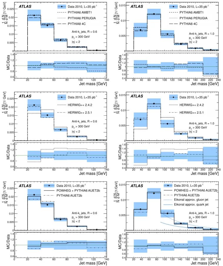
FIG. 6 (color online). The jet mass distributions for leadingpT, anti-ktR¼0:6(left) andR¼1:0(right) jets in the full 2010 data set, corrected for pileup and corrected to particle level. The data are compared to various tunes ofPYTHIA6 andPYTHIA8 (top),HERWIG ++2.4.2 and 2.5.1 (center) andPYTHIA AUET2Bwith and withoutPOWHEG(bottom). The eikonal approximation of NLO QCD for quark and gluon jets is also included for theR¼1:0case (right, bottom). The shaded bands indicate the sum of statistical and systematic uncertainties.
Ci¼A part i Adet i : (18)
The size of the corrections varies quite significantly between observables and between bins, being around 20% for mass (5%–10% around the peak, 20% elsewhere) and width (30% in the peak for R¼0:6 jets, 1%–5% elsewhere). The corrections for eccentricity are below 10% in the peak, increasing to 40% in the most sparsely populated bin. The detector corrections for angularity and planar flow are smaller, generally around 0%–5%.
VII. SYSTEMATIC UNCERTAINTIES
The experimental systematic uncertainties can be di-vided into three categories: how well modeled the observ-ables are in Monte Carlo simulations (Sec. VII A), the modeling of the detector material and cluster reconstruc-tion (Sec.VII B) and the pileup corrections (Sec. VII C). These are evaluated by determining the difference in the factors obtained after the application of systematic varia-tions to the samples used in the correction for detector effects. The dominant sources of uncertainty, described in detail below, arise from varying the cluster energy scale (CES) and from the differences found when the calculation of detector corrections is done using the HERWIG++ Monte Carlo sample in place of PYTHIA AMBT1. These dominant effects are shown in Fig.4forR¼0:6jets and Fig.5forR¼1:0jets.
A. Uncertainties on the Monte Carlo model
The distributions are corrected to particle level using the correction factorsCidetermined with a specific Monte Carlo generator, inclusive of parton shower, hadro-nization and UE model, which in this case isPYTHIAwith the AMBT1 tune. To determine the uncertainty introduced on the final measurement by choosing this particular model to calculate the detector correction factors, the differences in these Ci are found when the PYTHIA AMBT1 tune is replaced with the PERUGIA2010 tune, and with HERWIG++ (2.4.2).
A primary source of the uncertainty on the mass mea-surements is due to the observed differences in the detector correction factors between HERWIG++ and PYTHIA, with uncertainties ranging between 10% and 20% as shown in Figs.4and5.
B. Uncertainties on the detector material description and cluster reconstruction
Performance studies [50] have shown that there is excellent agreement between the measured positions of clusters and tracks in data, indicating no systematic mis-alignment between the calorimeter and inner detector. The Monte Carlo modeling of the position of clusters with respect to tracks is also good, indicating that the
detector simulation models the calorimeter position reso-lution adequately; however, there remains a small dis-crepancy between data and Monte Carlo in the mean and RMS of the track-cluster separation. This source of uncertainty is taken into account by (Gaussian) smearing the positions of simulated clusters inandby 5 mrad. This smearing is done independently inand, and the impact on the measurement of the correction factors for each observable, bin by bin, is quantified by taking the difference, Ci, between the correction factors obtained before and after the position smearing. Smearing the positions in and results in small Ci for mass and shapes alike, introducing uncertainties that do not exceed 5% in any bin.
The variation on the CES follows the procedure used by previous studies [3] according to
pclus;new ¼pclus
10:05
1þp 1:5
T=GeV
; (19)
where pclus is each component of the cluster’s four-momentum and pT is the cluster pT in GeV. The CES is varied up and down independently for each momen-tum component of each cluster, and the correction fac-tors are recalculated in each case as before. The CES is a large source of systematic uncertainty in the measure-ment of mass (of order 20% across the mass range) and width (of order 10% beyond the first two bins). The effects of varying the CES are, in general, smaller for the eccentricity, planar flow and angularity measurements, all
TABLE II. Measured values of the anti-kt R¼1:0 jet mass distribution given with their statistical and systematic uncertainties.
Bin (GeV) N1 dMdNstatsysð104Þ½ 1 GeV
20–55 691þ23
24
55–90 1221þ17
18
90–125 56113
125–160 22:60:4þ3:2
3:4
160–200 9:00:2þ2:4
2:3
200–240 4:30:2þ2:1
1:8
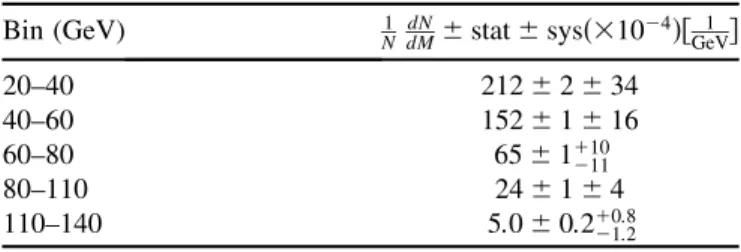
TABLE I. Measured values of the anti-kt R¼0:6 jet mass distribution given with their statistical and systematic uncertainties.
Bin (GeV) N1 dMdNstatsysð104Þ½ 1 GeV
20–40 212234
40–60 152116
60–80 651þ10
11
80–110 2414
110–140 5:00:2þ0:8
1:2
FIG. 7 (color online). The jet width distributions for leadingpT, anti-ktR¼0:6(left) andR¼1:0(right) jets in the full 2010 data set, corrected for pileup and corrected to particle level.
of which are made on high-mass jets only. The effects of varying the CES on all observables are shown with the label Eclus in Fig. 4 for R¼0:6 jets and Fig. 5 for
R¼1:0jets.
The uncertainty introduced as a result of losing energy due to dead material in the detector is taken into account by discarding a fraction of low energy (E <2:5 GeV) clus-ters, following the technique and utilizing the observations of a previous study of the single hadron response atpffiffiffis
¼ 900 GeV[51]. Clusters are not included in jet reconstruc-tion if they satisfy
r PðE0Þ e2E; (20)
where r is a random number r2 ð0;1, PðE0Þ is the measured uncertainty (28%) on the probability that a par-ticle does not leave a cluster in the calorimeter, andEis the cluster energy in GeV. The impact on the measurement of each observable is quantified by comparing the correction factors before and after this dropping of low energy clus-ters. The impact of this variation is small, resulting in a contribution to the systematic uncertainty of less than a few percent in all measurements.
C. Uncertainties on the pileup corrections There is a statistical uncertainty on the fitfðx; pT; MÞ
describing the pileup correction x for observable x in
R¼0:6 jets. Dedicated studies have shown that the pa-rametrizations of the pileup corrections in data and in PYTHIA AMBT1Monte Carlo with simulated pileup agree, within the statistical uncertainties, for jets across the pT range considered. The statistical uncertainties on these fits are accounted for by implementingþ1and1 varia-tions independently, as shown for mass in Fig. 2. The correction factors are recalculated, and in each case the difference is taken as a contribution to the systematic uncertainty on the measurement. This is a small contribu-tion to the overall systematic uncertainty on the measure-ments, contributing at most a few percent in bins that are statistically limited, and is a negligible (<1%) effect elsewhere.
ForR¼1:0jets, the correction factors are scaled using the phenomenological predictions described in Sec. VI B. These scaling factors are also calculated in data and in PYTHIA AMBT1 Monte Carlo with simulated pileup; good agreement is observed, indicating that the effect of pileup on jets is well modeled. In the case of mass and width, where there is a phenomenological prediction for the scal-ing, this prediction is used for the determination of the nominal scaling factors and the variation is taken from the scaling factors found in data. In the case of eccentricity there is no phenomenological prediction for the scaling of the pileup corrections withR, so the behavior observed in data is used. The R scaling of the pileup corrections for eccentricity is dependent on jet mass, so the variations found in data across the mass range are taken as the systematic variations.
The uncertainties introduced by the pileup corrections contribute a small amount (in general 1%–2%) to the total systematic uncertainties on the mass, width and eccentricity.
The sources of systematic uncertainty described above are added in quadrature with the statistical uncertainty in each bin and symmetrized where appropriate (the contri-butions from the cluster energy scale and parametrization of the pileup corrections are determined separately for upward and downward fluctuations, and so are not symmetrized).
VIII. RESULTS
The distributions of jet characteristics presented in this section are corrected for detector effects and are com-pared to Monte Carlo predictions at the particle level. In the case of mass and 2, comparison is also made between data and the eikonal approximation [46] of NLO QCD. The results shown here are available in HEPDATA [52,53] and the analysis and data are available as a RIVET[54,55] routine.
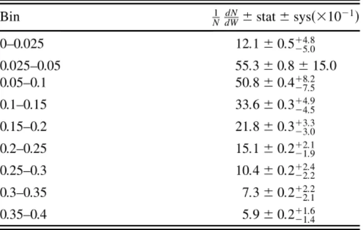
TABLE III. Measured values of the anti-kt R¼0:6 jet width distribution given with their statistical and systematic uncertainties.
Bin 1
NdWdNstatsysð10
1
Þ
0–0.025 61:11:2þ8:2
8:5
0.025–0.05 1061þ12
11
0.05–0.1 55:30:4þ10
9
0.1–0.15 26:40:3þ4
3
0.15–0.2 14:00:32
0.2–0.25 7:70:2þ1:3
1:2
0.25–0.3 4:00:2þ0:9
0:7
TABLE IV. Measured values of the anti-kt R¼1:0 jet width distribution given with their statistical and systematic uncertainties.
Bin 1
NdWdNstatsysð10
1
Þ
0–0.025 12:10:5þ4:8
5:0
0.025–0.05 55:30:815:0
0.05–0.1 50:80:4þ8:2
7:5
0.1–0.15 33:60:3þ4:9
4:5
0.15–0.2 21:80:3þ3:3
3:0
0.2–0.25 15:10:2þ2:1
1:9
0.25–0.3 10:40:2þ2:4
2:2
0.3–0.35 7:30:2þ2:2
2:1
0.35–0.4 5:90:2þ1:6
1:4
FIG. 8 (color online). The jet eccentricity distributions for high-mass (M >100 GeV), leadingpT, anti-kt R¼0:6(left) andR¼
1:0(right) jets in the full 2010 data set, corrected for pileup and corrected to particle level.
A. Jet mass
The jet mass distributions are shown in Fig.6 for jets satisfying pT>300 GeV and jj<2, corrected to the particle level, and the corresponding numerical values are given in TablesIandII.
In the case ofR¼1:0jets, the data are compared to the calculations for jet masses derived at NLO QCD in the eikonal approximation:
J’S
4Cc
M log
1
z tan
R
2
ffiffiffiffiffiffiffiffiffiffiffiffiffiffi
4z2
p
; (21)
whereJis the value of the jet mass distribution atM,Sis the strong coupling constant,z¼M=pT, c represents the flavor of the parton which initiated the jet andCc¼43(3) for quarks (gluons). The strong coupling constant is calcu-lated using thePYTHIAprediction of the average jetpT’
365 GeV and has the value of S¼0:0994. Theoretical uncertainties for such predictions are sizable (more than 30%) [46] in the region above the mass peak. The lower mass regionM&90 GeVis strongly affected by nonper-turbative physics and as such cannot be predicted by such calculations. The size and shape of the high-mass tail is in rough agreement with the analytical eikonal approximation for NLO QCD for jet masses above 90 GeV, with most of the data points lying between the predictions for quark-initiated and gluon-quark-initiated jets. QCD LO calculations predict that the jets in this sample should be roughly 50% quark initiated, with this fraction increasing as a function of the jetpTcut [56].
Also included in Fig. 6 are a number of PYTHIA, HERWIG++, and POWHEG predictions for the jet mass distributions. Unlike the analytical calculation discussed
above, the Monte Carlo predictions are meaningful down to the low mass region due to the inclusion of soft radiation and hadronization. The PYTHIA calculation describes the data well. The HERWIG++2.4.2 prediction indicates a sig-nificant shift to a higher jet mass that is inconsistent with
TABLE VI. Measured values of the eccentricity distribution for anti-kt R¼1:0 jets with M >100 GeV, given with their statistical and systematic uncertainties.
Bin 1
NdNdEstatsysð10 1Þ
0–0.2 0:80:10:3
0.2–0.4 4:20:20:9
0.4–0.6 9:80:3þ1:2
1:4
0.6–0.8 17:20:4þ2:0
2:2
0.8–1.0 18:60:4þ2:8
2:7
TABLE V. Measured values of the eccentricity distribution for anti-ktR¼0:6jets withM >100 GeV, given with their statis-tical and systematic uncertainties.
Bin N1 dNdEstatsysð101Þ
0–0.2 0:20:10:2
0.2–0.4 1:10:30:6
0.4–0.6 5:10:7þ1:5
1:3
0.6–0.8 11:00:9þ1:3
1:4
0.8–1.0 32:91:7þ2:4
2:7
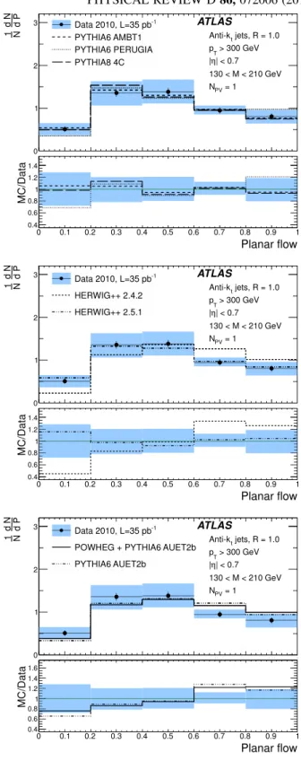
FIG. 9 (color online). The jet planar flow distributions for high-mass (130< M <210 GeV), leading pT, anti-kt R¼1:0 jets inNPV¼1events, corrected to particle level.
the data and the other Monte Carlo predictions, while the more recent HERWIG++ 2.5.1 generator is in much better agreement with the data. POWHEG+PYTHIA is in good agreement with data within systematic uncertainties across the whole mass range.
B. Width
The jet width distributions are shown in Fig.7for anti-kt
jets reconstructed with distance parameters ofR¼0:6and 1.0, and the corresponding numerical values are given in TablesIIIandIV. There is significant variation between the different Monte Carlo predictions in the first bin, beyond which there is good agreement between the distribution measured in data and all the predictions.
C. Eccentricity
The eccentricity distributions for high-mass (M > 100 GeV) anti-ktjets reconstructed with distance parame-ters of R¼0:6 and R¼1:0 are shown in Fig. 8, and the corresponding numerical values are given in TablesV
and VI. The Monte Carlo predictions generally describe the data, while some small discrepancies can be observed between the various predictions and between predictions and data.
D. Planar flow
The planar flow distributions are shown only for events known to be uncontaminated by pileup, corresponding to events with NPV¼1. These distributions are shown in Fig. 9 for jets reconstructed with the anti-kt algorithm with R¼1:0 for the mass range 130< M <210 GeV, and the corresponding numerical values are given in Table VII. The HERWIG++ 2.4.2 generator predicts jets with a more planar, isotropic energy distribution than is observed in data, while version 2.5.1 provides a very accu-rate description of the planar flow. The variousPYTHIAand POWHEG Monte Carlo predictions also describe the data well, within uncertainties.
E. Angularity
The2 distribution for anti-ktR¼0:6jets in the mass region 100< M <130 GeV is presented in Fig.10, and
TABLE VII. Measured values of the planar flow distribution for anti-ktR¼1:0jets inNPV¼1events with130< M <210 GeV,
given with their statistical and systematic uncertainties.
Bin 1
NdNdPstatsysð101Þ
0–0.2 5:10:71:4
0.2–0.4 13:60:9þ2:7
3:0
0.4–0.6 13:80:9þ2:9
2:7
0.6–0.8 9:50:8þ1:2
0:9
0.8–1.0 8:10:7þ1:5
1:7
FIG. 10 (color online). The angularity 2 distributions for
leading pT, anti-kt R¼0:6jets in the mass range 100< M <
130 GeV, in the full 2010 data set, corrected to particle level. The peak and maximum positions predicted by the small-angle approximation of Eq. (10) are indicated.
the corresponding numerical values are given in Table VIII. The QCD predictions for the peak position and the maximum value of2 [13], calculated using the averageshMi ¼111 GeVandhpTi ¼434 GeVof the jets in this kinematic region, are also shown on the distribu-tions. Good agreement is observed between the data and the Monte Carlo simulation for the shape of the 2 distribution.
The comparison between data and the analytic QCD prediction is limited by the intrinsic resolution of the data distribution; however, there is good agreement be-tween theory and data within these limitations. The posi-tion of the peak of the distribuposi-tion,peak2 , indicates that the majority of jets in this data set can be described by a two-body substructure in a symmetric pT configuration with respect to the jet axis. No jets are observed above the small-angle kinematic limit,max
2 .
IX. CONCLUSIONS
The properties of high-pT (>300 GeV) jets recon-structed with the anti-kt jet algorithm have been studied inppcollisions at a center-of-mass energy of 7 TeV. There is good agreement between data and PYTHIA for all ob-servables, and the POWHEG+PYTHIA prediction describes the mass distribution well for jets with M >20 GeV. HERWIG++2.4.2 predicts jets with a slightly more isotropic
energy flow and higher mass than observed in data, while HERWIG++2.5.1 predictions are in good agreement with the data. The angularity measurement of high-mass jets agrees with the small-angle QCD approximations.
ACKNOWLEDGMENTS
We thank CERN for the very successful operation of the LHC, as well as the support staff from our institutions without whom ATLAS could not be operated efficiently. We acknowledge the support of ANPCyT, Argentina; YerPhI, Armenia; ARC, Australia; BMWF, Austria; ANAS, Azerbaijan; SSTC, Belarus; CNPq and FAPESP, Brazil; NSERC, NRC and CFI, Canada; CERN; CONICYT, Chile; CAS, MOST and NSFC, China; COLCIENCIAS, Colombia; MSMT CR, MPO CR and
VSC CR, Czech Republic; DNRF, DNSRC and
Lundbeck Foundation, Denmark; EPLANET and ERC, European Union; IN2P3-CNRS, CEA-DSM/IRFU, France; GNAS, Georgia; BMBF, DFG, HGF, MPG and AvH Foundation, Germany; GSRT, Greece; ISF, MINERVA, GIF, DIP and Benoziyo Center, Israel; INFN, Italy; MEXT and JSPS, Japan; CNRST, Morocco; FOM and NWO, Netherlands; RCN, Norway; MNiSW, Poland; GRICES and FCT, Portugal; MERYS (MECTS), Romania; MES of Russia and ROSATOM, Russian Federation; JINR; MSTD, Serbia; MSSR, Slovakia; ARRS and MVZT, Slovenia; DST/NRF, South Africa; MICINN, Spain; SRC and Wallenberg Foundation, Sweden; SER, SNSF and Cantons of Bern and Geneva, Switzerland; NSC, Taiwan; TAEK, Turkey; STFC, the Royal Society and Leverhulme Trust, United Kingdom; DOE and NSF, United States of America. The crucial computing support from all WLCG partners is acknowledged gratefully, in particular from CERN and the ATLAS Tier-1 facilities at TRIUMF (Canada), NDGF (Denmark, Norway, Sweden), CC-IN2P3 (France), KIT/GridKA (Germany), INFN-CNAF (Italy), NL-T1 (Netherlands), PIC (Spain), ASGC (Taiwan), RAL (UK) and BNL (USA) and in the Tier-2 facilities worldwide.
[1] ATLAS Collaboration,Phys. Rev. D86, 014022 (2012). [2] CMS Collaboration,Phys. Lett. B700, 187 (2011). [3] ATLAS Collaboration,Phys. Rev. D83, 052003 (2011). [4] CMS Collaboration,J. High Energy Phys. 06 (2012) 160. [5] ATLAS Collaboration, J. High Energy Phys. 05 (2012)
128.
[6] ATLAS Collaboration,New J. Phys.13, 053044 (2011). [7] CMS Collaboration, Phys. Rev. Lett. 106, 201804
(2011).
[8] A. Altheimeret al.,J. Phys. G39, 063001 (2012).
[9] J. Butterworth, A. R. Davison, M. Rubin, and G. P. Salam, Phys. Rev. Lett.100, 242001 (2008).
[10] L. Almeida, S. Lee, G. Perez, G. Sterman, I. Sung, and J. Virzi,Phys. Rev. D79, 074017 (2009).
[11] Y. Cui, Z. Han, and M. Schwartz,Phys. Rev. D83, 074023 (2011).
[12] S. Chekanov and J. Proudfoot,Phys. Rev. D81, 114038 2010.
[13] T. Aaltonenet al.(CDF Collaboration),Phys. Rev. D85, 091101 (2012).
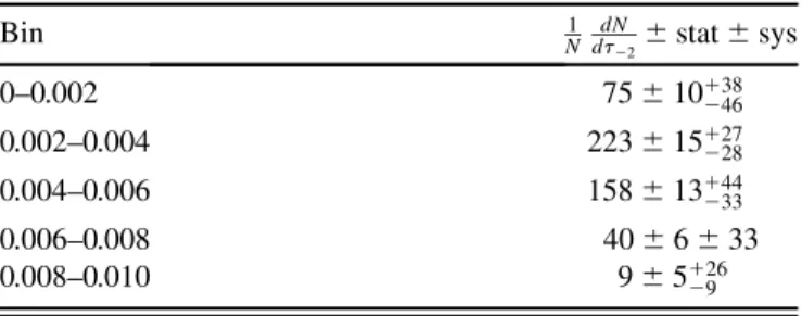
TABLE VIII. Measured values of the angularity2
distribu-tion for anti-kt R¼0:6 jets with 100< M <130 GeV, given with their statistical and systematic uncertainties.
Bin N1 ddN
2statsys
0–0.002 7510þ38
46
0.002–0.004 22315þ27
28
0.004–0.006 15813þ44
33
0.006–0.008 40633
0.008–0.010 95þ26
9
[14] T. Plehn, G. Salam, and M. Spannowsky,Phys. Rev. Lett. 104, 111801 (2010).
[15] ATLAS Collaboration,New J. Phys.13, 053033 (2011). [16] ATLAS Collaboration, Report No.
ATLAS-CONF-2010-069, 2010 (https://cdsweb.cern.ch/record/1281344). [17] ATLAS Collaboration,JINST3, S08003 (2008).
[18] T. Sjostrand, S. Mrenna, and P. Skands, J. High Energy Phys. 05 (2006) 026.
[19] ATLAS Collaboration, Report No. ATLAS-CONF-2010-031, 2010 (https://cdsweb.cern.ch/record/1277665). [20] A. Sherstnev and R. Thorne, Eur. Phys. J. C 55, 553
(2008).
[21] B. Andersson, G. Gustafson, G. Ingelman, and T. Sjo¨strand,Phys. Rep.97, 31 (1983).
[22] B. Andersson, G. Gustafson, and G. Soderberg,Z. Phys. C 20, 317 (1983).
[23] M. Bowler,Z. Phys. C11, 169 (1981).
[24] ATLAS Collaboration,Phys. Lett. B688, 21 (2010). [25] ATLAS Collaboration, Report No.
ATLAS-CONF-2010-024, 2010 (https://cdsweb.cern.ch/record/1277656). [26] P. Skands,Phys. Rev. D82, 074018 (2010).
[27] ATLAS Collaboration,Phys. Rev. D84, 054001 (2011). [28] H. L. Lai, J. Huston, S. Kuhlmann, J. Morfin, F. Olness,
J. F. Owens, J. Pumplin, and W. K. Tung,Eur. Phys. J. C 12, 375 (2000).
[29] M. Bahret al.,Eur. Phys. J. C58, 639 (2008).
[30] ATLAS Collaboration, Report No. ATL-PHYS-PUB-2011-009, 2011 (https://cdsweb.cern.ch/record/1363300). [31] ATLAS Collaboration, Report No. ATL-PHYS-PUB-2011-014, 2011 (https://cdsweb.cern.ch/record/1400677). [32] T. Sjostrand, S. Mrenna, and P. Skands, Comput. Phys.
Commun.178, 852 (2008).
[33] S. Alioli, K. Hamilton, P. Nason, C. Oleari, and E. Re,J. High Energy Phys. 04 (2011) 081.
[34] P. Nason,J. High Energy Phys. 11 (2004) 040.
[35] S. Frixione, P. Nason, and C. Oleari,J. High Energy Phys. 11 (2007) 070.
[36] S. Alioli, P. Nason, C. Oleari, and E. Re,J. High Energy Phys. 06 (2010) 043.
[37] ATLAS Collaboration,Eur. Phys. J. C70, 823 (2010). [38] S. Agostinelliet al.,Nucl. Instrum. Methods Phys. Res.,
Sect. A506, 250 (2003).
[39] G. Folger and J. Wellisch,arXiv:nucl-th/0306007. [40] H. W. Bertini,Phys. Rev.188, 1711 (1969).
[41] ATLAS Collaboration,Eur. Phys. J. C71, 1630 (2011). [42] ATLAS Collaboration, Report No.
ATLAS-CONF-2011-011, 2011 (https://cdsweb.cern.ch/record/1334563). [43] ATLAS Collaboration, Report No. ATL-LARG-
PUB-2008-002, 2008 (https://cdsweb.cern.ch/record/1099735). [44] M. Cacciari, G. Salam, and G. Soyez, J. High Energy
Phys. 04 (2008) 063.
[45] ATLAS Collaboration,arXiv:1112.6426[Eur. Phys. J. C (to be published)].
[46] L. Almeida, S. Lee, G. Perez, I. Sung, and J. Virzi,Phys. Rev. D79, 074012 (2009).
[47] J. Thaler and L.-T. Wang,J. High Energy Phys. 7 (2008) 092. [48] R. Alon, E. Duchovni, G. Perez, A. Pranko, and P. Sinervo,
Phys. Rev. D84, 114025 (2011).
[49] M. Dasgupta, L. Magnea, and G. Salam,J. High Energy Phys. 02 (2008) 055.
[50] ATLAS Collaboration,Phys. Rev. Lett.106, 172002, 2011. [51] ATLAS Collaboration,arXiv:1203.1302[Eur. Phys. J. C
(to be published)].
[52] A. Buckley and M. Whalley, Proc. Sci., ACAT2010 (2010) 067 [http://arxiv.org/abs/1006.0517v2].
[53] HEPDATA: ATLAS measurements of the properties of jets for boosted particle searches, http://hepdata.cedar.ac.uk/ view/red4992.
[54] A. Buckleyet al.,arXiv:1003.0694v6.
[55] RIVETroutine: ATLAS measurements of the properties of jets for boosted particle searches,http://rivet.hepforge.org/ analyses.
[56] J. Gallichio and M. Schwartz, J. High Energy Phys. 10 (2011) 103.
G. Aad,47B. Abbott,110J. Abdallah,11S. Abdel Khalek,114A. A. Abdelalim,48O. Abdinov,10B. Abi,111 M. Abolins,87O. S. AbouZeid,157H. Abramowicz,152H. Abreu,135E. Acerbi,88a,88bB. S. Acharya,163a,163b L. Adamczyk,37D. L. Adams,24T. N. Addy,55J. Adelman,175S. Adomeit,97P. Adragna,74T. Adye,128S. Aefsky,22
J. A. Aguilar-Saavedra,123b,bM. Aharrouche,80S. P. Ahlen,21F. Ahles,47A. Ahmad,147M. Ahsan,40 G. Aielli,132a,132bT. Akdogan,18aT. P. A. A˚ kesson,78G. Akimoto,154A. V. Akimov,93A. Akiyama,65M. S. Alam,1
M. A. Alam,75J. Albert,168S. Albrand,54M. Aleksa,29I. N. Aleksandrov,63F. Alessandria,88aC. Alexa,25a G. Alexander,152G. Alexandre,48T. Alexopoulos,9M. Alhroob,163a,163cM. Aliev,15G. Alimonti,88aJ. Alison,119
B. M. M. Allbrooke,17P. P. Allport,72S. E. Allwood-Spiers,52J. Almond,81A. Aloisio,101a,101bR. Alon,171 A. Alonso,78B. Alvarez Gonzalez,87M. G. Alviggi,101a,101bK. Amako,64C. Amelung,22V. V. Ammosov,127,a A. Amorim,123a,cN. Amram,152C. Anastopoulos,29L. S. Ancu,16N. Andari,114T. Andeen,34C. F. Anders,57b G. Anders,57aK. J. Anderson,30A. Andreazza,88a,88bV. Andrei,57aX. S. Anduaga,69P. Anger,43A. Angerami,34
F. Anghinolfi,29A. Anisenkov,106N. Anjos,123aA. Annovi,46A. Antonaki,8M. Antonelli,46A. Antonov,95 J. Antos,143bF. Anulli,131aS. Aoun,82L. Aperio Bella,4R. Apolle,117,dG. Arabidze,87I. Aracena,142Y. Arai,64 A. T. H. Arce,44S. Arfaoui,147J-F. Arguin,14E. Arik,18a,aM. Arik,18aA. J. Armbruster,86O. Arnaez,80V. Arnal,79
C. Arnault,114A. Artamonov,94G. Artoni,131a,131bD. Arutinov,20S. Asai,154R. Asfandiyarov,172S. Ask,27 B. A˚ sman,145a,145bL. Asquith,5K. Assamagan,24A. Astbury,168B. Aubert,4E. Auge,114K. Augsten,126 M. Aurousseau,144aG. Avolio,162R. Avramidou,9D. Axen,167G. Azuelos,92,eY. Azuma,154M. A. Baak,29 G. Baccaglioni,88aC. Bacci,133a,133bA. M. Bach,14H. Bachacou,135K. Bachas,29M. Backes,48M. Backhaus,20
E. Badescu,25aP. Bagnaia,131a,131bS. Bahinipati,2Y. Bai,32aD. C. Bailey,157T. Bain,157J. T. Baines,128 O. K. Baker,175M. D. Baker,24S. Baker,76E. Banas,38P. Banerjee,92Sw. Banerjee,172D. Banfi,29A. Bangert,149
V. Bansal,168H. S. Bansil,17L. Barak,171S. P. Baranov,93A. Barbaro Galtieri,14T. Barber,47E. L. Barberio,85 D. Barberis,49a,49bM. Barbero,20D. Y. Bardin,63T. Barillari,98M. Barisonzi,174T. Barklow,142N. Barlow,27
B. M. Barnett,128R. M. Barnett,14A. Baroncelli,133aG. Barone,48A. J. Barr,117F. Barreiro,79
J. Barreiro Guimara˜es da Costa,56P. Barrillon,114R. Bartoldus,142A. E. Barton,70V. Bartsch,148R. L. Bates,52 L. Batkova,143aJ. R. Batley,27A. Battaglia,16M. Battistin,29F. Bauer,135H. S. Bawa,142,fS. Beale,97T. Beau,77 P. H. Beauchemin,160R. Beccherle,49aP. Bechtle,20H. P. Beck,16A. K. Becker,174S. Becker,97M. Beckingham,137
K. H. Becks,174A. J. Beddall,18cA. Beddall,18cS. Bedikian,175V. A. Bednyakov,63C. P. Bee,82M. Begel,24 S. Behar Harpaz,151M. Beimforde,98C. Belanger-Champagne,84P. J. Bell,48W. H. Bell,48G. Bella,152 L. Bellagamba,19aF. Bellina,29M. Bellomo,29A. Belloni,56O. Beloborodova,106,gK. Belotskiy,95O. Beltramello,29
O. Benary,152D. Benchekroun,134aK. Bendtz,145a,145bN. Benekos,164Y. Benhammou,152E. Benhar Noccioli,48 J. A. Benitez Garcia,158bD. P. Benjamin,44M. Benoit,114J. R. Bensinger,22K. Benslama,129S. Bentvelsen,104
D. Berge,29E. Bergeaas Kuutmann,41N. Berger,4F. Berghaus,168E. Berglund,104J. Beringer,14P. Bernat,76 R. Bernhard,47C. Bernius,24T. Berry,75C. Bertella,82A. Bertin,19a,19bF. Bertolucci,121a,121bM. I. Besana,88a,88b
G. J. Besjes,103N. Besson,135S. Bethke,98W. Bhimji,45R. M. Bianchi,29M. Bianco,71a,71bO. Biebel,97 S. P. Bieniek,76K. Bierwagen,53J. Biesiada,14M. Biglietti,133aH. Bilokon,46M. Bindi,19a,19bS. Binet,114 A. Bingul,18cC. Bini,131a,131bC. Biscarat,177U. Bitenc,47K. M. Black,21R. E. Blair,5J.-B. Blanchard,135 G. Blanchot,29T. Blazek,143aC. Blocker,22J. Blocki,38A. Blondel,48W. Blum,80U. Blumenschein,53 G. J. Bobbink,104V. B. Bobrovnikov,106S. S. Bocchetta,78A. Bocci,44C. R. Boddy,117M. Boehler,41J. Boek,174
N. Boelaert,35J. A. Bogaerts,29A. Bogdanchikov,106A. Bogouch,89,aC. Bohm,145aJ. Bohm,124V. Boisvert,75 T. Bold,37V. Boldea,25aN. M. Bolnet,135M. Bomben,77M. Bona,74M. Bondioli,162M. Boonekamp,135 C. N. Booth,138S. Bordoni,77C. Borer,16A. Borisov,127G. Borissov,70I. Borjanovic,12aM. Borri,81S. Borroni,86 V. Bortolotto,133a,133bK. Bos,104D. Boscherini,19aM. Bosman,11H. Boterenbrood,104D. Botterill,128J. Bouchami,92 J. Boudreau,122E. V. Bouhova-Thacker,70D. Boumediene,33C. Bourdarios,114N. Bousson,82A. Boveia,30J. Boyd,29
I. R. Boyko,63I. Bozovic-Jelisavcic,12bJ. Bracinik,17P. Branchini,133aA. Brandt,7G. Brandt,117O. Brandt,53 U. Bratzler,155B. Brau,83J. E. Brau,113H. M. Braun,174,aS. F. Brazzale,163a,163cB. Brelier,157J. Bremer,29 K. Brendlinger,119R. Brenner,165S. Bressler,171D. Britton,52F. M. Brochu,27I. Brock,20R. Brock,87E. Brodet,152 F. Broggi,88aC. Bromberg,87J. Bronner,98G. Brooijmans,34T. Brooks,75W. K. Brooks,31bG. Brown,81H. Brown,7
P. A. Bruckman de Renstrom,38D. Bruncko,143bR. Bruneliere,47S. Brunet,59A. Bruni,19aG. Bruni,19a M. Bruschi,19aT. Buanes,13Q. Buat,54F. Bucci,48J. Buchanan,117P. Buchholz,140R. M. Buckingham,117
A. G. Buckley,45S. I. Buda,25aI. A. Budagov,63B. Budick,107V. Bu¨scher,80L. Bugge,116O. Bulekov,95 A. C. Bundock,72M. Bunse,42T. Buran,116H. Burckhart,29S. Burdin,72T. Burgess,13S. Burke,128E. Busato,33
P. Bussey,52C. P. Buszello,165B. Butler,142J. M. Butler,21C. M. Buttar,52J. M. Butterworth,76W. Buttinger,27 S. Cabrera Urba´n,166D. Caforio,19a,19bO. Cakir,3aP. Calafiura,14G. Calderini,77P. Calfayan,97R. Calkins,105 L. P. Caloba,23aR. Caloi,131a,131bD. Calvet,33S. Calvet,33R. Camacho Toro,33P. Camarri,132a,132bD. Cameron,116 L. M. Caminada,14S. Campana,29M. Campanelli,76V. Canale,101a,101bF. Canelli,30,hA. Canepa,158aJ. Cantero,79
R. Cantrill,75L. Capasso,101a,101bM. D. M. Capeans Garrido,29I. Caprini,25aM. Caprini,25aD. Capriotti,98 M. Capua,36a,36bR. Caputo,80R. Cardarelli,132aT. Carli,29G. Carlino,101aL. Carminati,88a,88bB. Caron,84 S. Caron,103E. Carquin,31bG. D. Carrillo Montoya,172A. A. Carter,74J. R. Carter,27J. Carvalho,123a,iD. Casadei,107
M. P. Casado,11M. Cascella,121a,121bC. Caso,49a,49b,aA. M. Castaneda Hernandez,172,jE. Castaneda-Miranda,172 V. Castillo Gimenez,166N. F. Castro,123aG. Cataldi,71aP. Catastini,56A. Catinaccio,29J. R. Catmore,29A. Cattai,29
G. Cattani,132a,132bS. Caughron,87P. Cavalleri,77D. Cavalli,88aM. Cavalli-Sforza,11V. Cavasinni,121a,121b F. Ceradini,133a,133bA. S. Cerqueira,23bA. Cerri,29L. Cerrito,74F. Cerutti,46S. A. Cetin,18bA. Chafaq,134a D. Chakraborty,105I. Chalupkova,125K. Chan,2B. Chapleau,84J. D. Chapman,27J. W. Chapman,86E. Chareyre,77
D. G. Charlton,17V. Chavda,81C. A. Chavez Barajas,29S. Cheatham,84S. Chekanov,5S. V. Chekulaev,158a G. A. Chelkov,63M. A. Chelstowska,103C. Chen,62H. Chen,24S. Chen,32cX. Chen,172A. Cheplakov,63 R. Cherkaoui El Moursli,134eV. Chernyatin,24E. Cheu,6S. L. Cheung,157L. Chevalier,135G. Chiefari,101a,101b
L. Chikovani,50a,aJ. T. Childers,29A. Chilingarov,70G. Chiodini,71aA. S. Chisholm,17R. T. Chislett,76 M. V. Chizhov,63G. Choudalakis,30S. Chouridou,136I. A. Christidi,76A. Christov,47D. Chromek-Burckhart,29 M. L. Chu,150J. Chudoba,124G. Ciapetti,131a,131bA. K. Ciftci,3aR. Ciftci,3aD. Cinca,33V. Cindro,73C. Ciocca,19a,19b
A. Ciocio,14M. Cirilli,86P. Cirkovic,12bM. Citterio,88aM. Ciubancan,25aA. Clark,48P. J. Clark,45W. Cleland,122 J. C. Clemens,82B. Clement,54C. Clement,145a,145bY. Coadou,82M. Cobal,163a,163cA. Coccaro,137J. Cochran,62
J. G. Cogan,142J. Coggeshall,164E. Cogneras,177J. Colas,4A. P. Colijn,104N. J. Collins,17C. Collins-Tooth,52 J. Collot,54T. Colombo,118a,118bG. Colon,83P. Conde Muin˜o,123aE. Coniavitis,117M. C. Conidi,11 S. M. Consonni,88a,88bV. Consorti,47S. Constantinescu,25aC. Conta,118a,118bG. Conti,56F. Conventi,101a,k M. Cooke,14B. D. Cooper,76A. M. Cooper-Sarkar,117K. Copic,14T. Cornelissen,174M. Corradi,19aF. Corriveau,84,l
A. Cortes-Gonzalez,164G. Cortiana,98G. Costa,88aM. J. Costa,166D. Costanzo,138T. Costin,30D. Coˆte´,29 L. Courneyea,168G. Cowan,75C. Cowden,27B. E. Cox,81K. Cranmer,107F. Crescioli,121a,121bM. Cristinziani,20
G. Crosetti,36a,36bR. Crupi,71a,71bS. Cre´pe´-Renaudin,54C.-M. Cuciuc,25aC. Cuenca Almenar,175 T. Cuhadar Donszelmann,138M. Curatolo,46C. J. Curtis,17C. Cuthbert,149P. Cwetanski,59H. Czirr,140
P. Czodrowski,43Z. Czyczula,175S. D’Auria,52M. D’Onofrio,72A. D’Orazio,131a,131b
M. J. Da Cunha Sargedas De Sousa,123aC. Da Via,81W. Dabrowski,37A. Dafinca,117T. Dai,86C. Dallapiccola,83 M. Dam,35M. Dameri,49a,49bD. S. Damiani,136H. O. Danielsson,29V. Dao,48G. Darbo,49aG. L. Darlea,25b
W. Davey,20T. Davidek,125N. Davidson,85R. Davidson,70E. Davies,117,dM. Davies,92A. R. Davison,76 Y. Davygora,57aE. Dawe,141I. Dawson,138R. K. Daya-Ishmukhametova,22K. De,7R. de Asmundis,101a S. De Castro,19a,19bS. De Cecco,77J. de Graat,97N. De Groot,103P. de Jong,104C. De La Taille,114H. De la Torre,79
F. De Lorenzi,62L. de Mora,70L. De Nooij,104D. De Pedis,131aA. De Salvo,131aU. De Sanctis,163a,163c A. De Santo,148J. B. De Vivie De Regie,114G. De Zorzi,131a,131bW. J. Dearnaley,70R. Debbe,24C. Debenedetti,45
B. Dechenaux,54D. V. Dedovich,63J. Degenhardt,119C. Del Papa,163a,163cJ. Del Peso,79T. Del Prete,121a,121b T. Delemontex,54M. Deliyergiyev,73A. Dell’Acqua,29L. Dell’Asta,21M. Della Pietra,101a,kD. della Volpe,101a,101b
M. Delmastro,4P. A. Delsart,54C. Deluca,104S. Demers,175M. Demichev,63B. Demirkoz,11,mJ. Deng,162 S. P. Denisov,127D. Derendarz,38J. E. Derkaoui,134dF. Derue,77P. Dervan,72K. Desch,20E. Devetak,147 P. O. Deviveiros,104A. Dewhurst,128B. DeWilde,147S. Dhaliwal,157R. Dhullipudi,24,nA. Di Ciaccio,132a,132b
L. Di Ciaccio,4A. Di Girolamo,29B. Di Girolamo,29S. Di Luise,133a,133bA. Di Mattia,172B. Di Micco,29 R. Di Nardo,46A. Di Simone,132a,132bR. Di Sipio,19a,19bM. A. Diaz,31aE. B. Diehl,86J. Dietrich,41T. A. Dietzsch,57a
S. Diglio,85K. Dindar Yagci,39J. Dingfelder,20C. Dionisi,131a,131bP. Dita,25aS. Dita,25aF. Dittus,29F. Djama,82 T. Djobava,50bM. A. B. do Vale,23cA. Do Valle Wemans,123a,oT. K. O. Doan,4M. Dobbs,84R. Dobinson,29,a
D. Dobos,29E. Dobson,29,pJ. Dodd,34C. Doglioni,48T. Doherty,52Y. Doi,64,aJ. Dolejsi,125I. Dolenc,73 Z. Dolezal,125B. A. Dolgoshein,95,aT. Dohmae,154M. Donadelli,23dM. Donega,119J. Donini,33J. Dopke,29
A. Doria,101aA. Dos Anjos,172A. Dotti,121a,121bM. T. Dova,69A. D. Doxiadis,104A. T. Doyle,52M. Dris,9 J. Dubbert,98S. Dube,14E. Duchovni,171G. Duckeck,97A. Dudarev,29F. Dudziak,62M. Du¨hrssen,29I. P. Duerdoth,81
L. Duflot,114M-A. Dufour,84M. Dunford,29H. Duran Yildiz,3aR. Duxfield,138M. Dwuznik,37F. Dydak,29 M. Du¨ren,51J. Ebke,97S. Eckweiler,80K. Edmonds,80C. A. Edwards,75N. C. Edwards,52W. Ehrenfeld,41 T. Eifert,142G. Eigen,13K. Einsweiler,14E. Eisenhandler,74T. Ekelof,165M. El Kacimi,134cM. Ellert,165S. Elles,4 F. Ellinghaus,80K. Ellis,74N. Ellis,29J. Elmsheuser,97M. Elsing,29D. Emeliyanov,128R. Engelmann,147A. Engl,97
B. Epp,60A. Eppig,86J. Erdmann,53A. Ereditato,16D. Eriksson,145aJ. Ernst,1M. Ernst,24J. Ernwein,135 D. Errede,164S. Errede,164E. Ertel,80M. Escalier,114C. Escobar,122X. Espinal Curull,11B. Esposito,46F. Etienne,82
A. I. Etienvre,135E. Etzion,152D. Evangelakou,53H. Evans,59L. Fabbri,19a,19bC. Fabre,29R. M. Fakhrutdinov,127 S. Falciano,131aY. Fang,172M. Fanti,88a,88bA. Farbin,7A. Farilla,133aJ. Farley,147T. Farooque,157S. Farrell,162
S. M. Farrington,117P. Farthouat,29P. Fassnacht,29D. Fassouliotis,8B. Fatholahzadeh,157A. Favareto,88a,88b L. Fayard,114S. Fazio,36a,36bR. Febbraro,33P. Federic,143aO. L. Fedin,120W. Fedorko,87M. Fehling-Kaschek,47 L. Feligioni,82D. Fellmann,5C. Feng,32dE. J. Feng,30A. B. Fenyuk,127J. Ferencei,143bW. Fernando,5S. Ferrag,52
J. Ferrando,52V. Ferrara,41A. Ferrari,165P. Ferrari,104R. Ferrari,118aD. E. Ferreira de Lima,52A. Ferrer,166 D. Ferrere,48C. Ferretti,86A. Ferretto Parodi,49a,49bM. Fiascaris,30F. Fiedler,80A. Filipcˇicˇ,73F. Filthaut,103 M. Fincke-Keeler,168M. C. N. Fiolhais,123a,iL. Fiorini,166A. Firan,39G. Fischer,41M. J. Fisher,108M. Flechl,47 I. Fleck,140J. Fleckner,80P. Fleischmann,173S. Fleischmann,174T. Flick,174A. Floderus,78L. R. Flores Castillo,172
M. J. Flowerdew,98T. Fonseca Martin,16A. Formica,135A. Forti,81D. Fortin,158aD. Fournier,114H. Fox,70 P. Francavilla,11S. Franchino,118a,118bD. Francis,29T. Frank,171S. Franz,29M. Fraternali,118a,118bS. Fratina,119
S. T. French,27C. Friedrich,41F. Friedrich,43R. Froeschl,29D. Froidevaux,29J. A. Frost,27C. Fukunaga,155 E. Fullana Torregrosa,29B. G. Fulsom,142J. Fuster,166C. Gabaldon,29O. Gabizon,171T. Gadfort,24S. Gadomski,48 G. Gagliardi,49a,49bP. Gagnon,59C. Galea,97E. J. Gallas,117V. Gallo,16B. J. Gallop,128P. Gallus,124K. K. Gan,108
Y. S. Gao,142,fA. Gaponenko,14F. Garberson,175M. Garcia-Sciveres,14C. Garcı´a,166J. E. Garcı´a Navarro,166 R. W. Gardner,30N. Garelli,29H. Garitaonandia,104V. Garonne,29J. Garvey,17C. Gatti,46G. Gaudio,118aB. Gaur,140 L. Gauthier,135P. Gauzzi,131a,131bI. L. Gavrilenko,93C. Gay,167G. Gaycken,20E. N. Gazis,9P. Ge,32dZ. Gecse,167
C. N. P. Gee,128D. A. A. Geerts,104Ch. Geich-Gimbel,20K. Gellerstedt,145a,145bC. Gemme,49aA. Gemmell,52 M. H. Genest,54S. Gentile,131a,131bM. George,53S. George,75P. Gerlach,174A. Gershon,152C. Geweniger,57a H. Ghazlane,134bN. Ghodbane,33B. Giacobbe,19aS. Giagu,131a,131bV. Giakoumopoulou,8V. Giangiobbe,11 F. Gianotti,29B. Gibbard,24A. Gibson,157S. M. Gibson,29D. Gillberg,28A. R. Gillman,128D. M. Gingrich,2,e J. Ginzburg,152N. Giokaris,8M. P. Giordani,163cR. Giordano,101a,101bF. M. Giorgi,15P. Giovannini,98P. F. Giraud,135 D. Giugni,88aM. Giunta,92P. Giusti,19aB. K. Gjelsten,116L. K. Gladilin,96C. Glasman,79J. Glatzer,47A. Glazov,41
K. W. Glitza,174G. L. Glonti,63J. R. Goddard,74J. Godfrey,141J. Godlewski,29M. Goebel,41T. Go¨pfert,43 C. Goeringer,80C. Go¨ssling,42S. Goldfarb,86T. Golling,175A. Gomes,123a,cL. S. Gomez Fajardo,41R. Gonc¸alo,75 J. Goncalves Pinto Firmino Da Costa,41L. Gonella,20S. Gonzalez,172S. Gonza´lez de la Hoz,166G. Gonzalez Parra,11 M. L. Gonzalez Silva,26S. Gonzalez-Sevilla,48J. J. Goodson,147L. Goossens,29P. A. Gorbounov,94H. A. Gordon,24 I. Gorelov,102G. Gorfine,174B. Gorini,29E. Gorini,71a,71bA. Gorisˇek,73E. Gornicki,38B. Gosdzik,41A. T. Goshaw,5
M. Gosselink,104M. I. Gostkin,63I. Gough Eschrich,162M. Gouighri,134aD. Goujdami,134cM. P. Goulette,48 A. G. Goussiou,137C. Goy,4S. Gozpinar,22I. Grabowska-Bold,37P. Grafstro¨m,29K-J. Grahn,41F. Grancagnolo,71a
S. Grancagnolo,15V. Grassi,147V. Gratchev,120N. Grau,34H. M. Gray,29J. A. Gray,147E. Graziani,133a O. G. Grebenyuk,120T. Greenshaw,72Z. D. Greenwood,24,nK. Gregersen,35I. M. Gregor,41P. Grenier,142 J. Griffiths,137N. Grigalashvili,63A. A. Grillo,136S. Grinstein,11Y. V. Grishkevich,96J.-F. Grivaz,114E. Gross,171 J. Grosse-Knetter,53J. Groth-Jensen,171K. Grybel,140D. Guest,175C. Guicheney,33A. Guida,71a,71bS. Guindon,53
U. Gul,52H. Guler,84,qJ. Gunther,124B. Guo,157J. Guo,34P. Gutierrez,110N. Guttman,152O. Gutzwiller,172 C. Guyot,135C. Gwenlan,117C. B. Gwilliam,72A. Haas,142S. Haas,29C. Haber,14H. K. Hadavand,39D. R. Hadley,17
P. Haefner,20F. Hahn,29S. Haider,29Z. Hajduk,38H. Hakobyan,176D. Hall,117J. Haller,53K. Hamacher,174 P. Hamal,112M. Hamer,53A. Hamilton,144b,rS. Hamilton,160L. Han,32bK. Hanagaki,115K. Hanawa,159M. Hance,14 C. Handel,80P. Hanke,57aJ. R. Hansen,35J. B. Hansen,35J. D. Hansen,35P. H. Hansen,35P. Hansson,142K. Hara,159 G. A. Hare,136T. Harenberg,174S. Harkusha,89D. Harper,86R. D. Harrington,45O. M. Harris,137K. Harrison,17 J. Hartert,47F. Hartjes,104T. Haruyama,64A. Harvey,55S. Hasegawa,100Y. Hasegawa,139S. Hassani,135S. Haug,16 M. Hauschild,29R. Hauser,87M. Havranek,20C. M. Hawkes,17R. J. Hawkings,29A. D. Hawkins,78D. Hawkins,162
T. Hayakawa,65T. Hayashi,159D. Hayden,75C. P. Hays,117H. S. Hayward,72S. J. Haywood,128M. He,32d S. J. Head,17V. Hedberg,78L. Heelan,7S. Heim,87B. Heinemann,14S. Heisterkamp,35L. Helary,4C. Heller,97 M. Heller,29S. Hellman,145a,145bD. Hellmich,20C. Helsens,11R. C. W. Henderson,70M. Henke,57aA. Henrichs,53
A. M. Henriques Correia,29S. Henrot-Versille,114C. Hensel,53T. Henß,174C. M. Hernandez,7 Y. Herna´ndez Jime´nez,166R. Herrberg,15G. Herten,47R. Hertenberger,97L. Hervas,29G. G. Hesketh,76 N. P. Hessey,104E. Higo´n-Rodriguez,166J. C. Hill,27K. H. Hiller,41S. Hillert,20S. J. Hillier,17I. Hinchliffe,14
E. Hines,119M. Hirose,115F. Hirsch,42D. Hirschbuehl,174J. Hobbs,147N. Hod,152M. C. Hodgkinson,138 P. Hodgson,138A. Hoecker,29M. R. Hoeferkamp,102J. Hoffman,39D. Hoffmann,82M. Hohlfeld,80M. Holder,140
S. O. Holmgren,145aT. Holy,126J. L. Holzbauer,87T. M. Hong,119L. Hooft van Huysduynen,107C. Horn,142 S. Horner,47J-Y. Hostachy,54S. Hou,150A. Hoummada,134aJ. Howard,117J. Howarth,81I. Hristova,15J. Hrivnac,114 T. Hryn’ova,4P. J. Hsu,80S.-C. Hsu,14Z. Hubacek,126F. Hubaut,82F. Huegging,20A. Huettmann,41T. B. Huffman,117 E. W. Hughes,34G. Hughes,70M. Huhtinen,29M. Hurwitz,14U. Husemann,41N. Huseynov,63,sJ. Huston,87J. Huth,56 G. Iacobucci,48G. Iakovidis,9M. Ibbotson,81I. Ibragimov,140L. Iconomidou-Fayard,114J. Idarraga,114P. Iengo,101a
O. Igonkina,104Y. Ikegami,64M. Ikeno,64D. Iliadis,153N. Ilic,157T. Ince,20J. Inigo-Golfin,29P. Ioannou,8 M. Iodice,133aK. Iordanidou,8V. Ippolito,131a,131bA. Irles Quiles,166C. Isaksson,165A. Ishikawa,65M. Ishino,66 R. Ishmukhametov,39C. Issever,117S. Istin,18aA. V. Ivashin,127W. Iwanski,38H. Iwasaki,64J. M. Izen,40V. Izzo,101a B. Jackson,119J. N. Jackson,72P. Jackson,142M. R. Jaekel,29V. Jain,59K. Jakobs,47S. Jakobsen,35T. Jakoubek,124
J. Jakubek,126D. K. Jana,110E. Jansen,76H. Jansen,29A. Jantsch,98M. Janus,47G. Jarlskog,78L. Jeanty,56 I. Jen-La Plante,30P. Jenni,29A. Jeremie,4P. Jezˇ,35S. Je´ze´quel,4M. K. Jha,19aH. Ji,172W. Ji,80J. Jia,147Y. Jiang,32b
M. Jimenez Belenguer,41S. Jin,32aO. Jinnouchi,156M. D. Joergensen,35D. Joffe,39M. Johansen,145a,145b K. E. Johansson,145aP. Johansson,138S. Johnert,41K. A. Johns,6K. Jon-And,145a,145bG. Jones,169R. W. L. Jones,70
T. J. Jones,72C. Joram,29P. M. Jorge,123aK. D. Joshi,81J. Jovicevic,146T. Jovin,12bX. Ju,172C. A. Jung,42 R. M. Jungst,29V. Juranek,124P. Jussel,60A. Juste Rozas,11S. Kabana,16M. Kaci,166A. Kaczmarska,38P. Kadlecik,35