Rev. Bras. Econ. vol.68 número3

(1)

Fernando N. de Oliveira

∗

, Myrian Petrassi

†

Contents: 1. Introduction; 2. Data; 3. Empirical Analysis; 4. Conclusion.

Keywords: Taylor Rule, Inflation Rate in the Short Run, Monetary Policy, Inflation Targeting. JEL Code: E3, E30, E31.

We analyze inflation persistence in several industrial and emerging countries in the recent past by implementing unit root tests in the presence of unknown structural breaks and by estimating reduced-form models of inflation dynamics. We select a very representative group of 23 industrial and 17 emerging economies. Our sample period is comprised of quarterly data and differs for each country. Our results indicate that inflation persistence is decreasing over time for the great majority of industrial economies. Many emerging economies, however, show increasing persistence and even a few have highly persistent inflationary processes. We also observe structural breaks in all inflation processes we study with the exception of the inflation processes of Germany and Austria. Our results are robust to different reduced forms of the inflation processes and different econometric techniques.

Analisamos a persistência da inflação em vários países industriais e emergentes no passado recente, por meio da implementação de testes de raiz unitária na presença de quebras estruturais desconhecidas e por meio da estimação de modelos de forma reduzida da dinâmica da inflação. Selecionamos um grupo representativo de 23 economias industriais e 17 economias emergentes. Nosso período amostral é composto por dados trimestrais e varia entre os países de nossa amostra. Nossos resultados indicam que a persistência da inflação diminui ao longo do tempo para a grande maioria das economias industriais. Muitas economias emergentes, no entanto, mostram aumento da persistência e, até mesmo, algumas dessas economias têm processos inflacionários altamente persistentes. Observamos, também, quebras estruturais em todos os processos de inflação que estudamos com exceção dos processos de inflação da Alemanha e da Áustria. Nossos resultados são robustos a diferentes formas reduzidas de processos de inflação e diferentes técnicas econométricas.

∗_Research _Department _of _Central _Bank _of _Brazil _Rio _de _Janeiro _and _Assistant _Professor _IBMEC/RJ. E-mail:fernando.nascimento@bcb.gov.br

(2)

1. INTRODUCTION

One of the most important characteristics of the dynamics of inflation is its degree of persistence. It is related to how quickly inflation reverts to its initial level after a shock. As Mishkin (2007) points out, if inflation is persistent, it increases the costs of monetary policy (in terms of product or unemployment)

to keep inflation under control.1

In the last years, both industrial and emerging economies have experienced important changes in the degree of their inflationary persistence. As Cechetti et alii (2007) show both the volatility and level of inflation has decreased in industrial economies. In these economies, the decades of 1960 and 1970 were considered periods of high and persistent inflation, while the more recent decades, 1990 and 2000, have low levels of inflation as well as low persistence.

Contrary to industrial countries, emerging economies have experienced high levels of inflations for a longer period. Some of these countries, such as Brazil, Argentina, Bolivia, Peru, Mexico, Israel, Poland

and Turkey, have had periods of hyperinflation in the last thirty years.2 _{Only recently, in the decade}

of 1990, the levels of inflation have started to decrease in these countries. This, in part, is due to the

important changes in the conduct of their macroeconomic policies.3 _{However, it is not clear if the}

decrease of the level of inflation has been accompanied by a reduction of their inflationary persistence. Our objective in this paper is to analyze empirically the inflation persistence of several industrial and emerging countries in the recent past. We select a very representative group of 23 industrial and 17 emerging economies. We want to answer the following questions: has inflation persistence decreased and been stable for industrial economies? has it decreased and been stable for emerging economies

that had and had not experienced hyperinflation in the recent past?4,5,6,7

Our results, in general terms, show that inflation persistence is decreasing over time for the great majority of industrial economies in our sample. Many emerging economies in our sample, however, show increasing persistence and even a few have very persistent inflationary processes over time. We also find that, with the exception of inflation in Germany and Austria, all others inflation processes present structural breaks, which indicates that they have not been stable through time.

1_{In a more formal way, we can define inflation persistence as the propensity of inflation to converge slowly towards its long run} equilibrium following a shock that has taken inflation away from this equilibrium.

2_{To define a hyperinflation country, in the first place, we choose a sample of countries that had at least three consecutive} quarters of 15% inflation. We also look at the recent monetary history of the country, search IMF country reports and anecdote facts about the country.

3_{As examples of some macroeconomic policies we can list: inflation targeting adoption, reduction of budget deficits,} improvement of financial regulation, trade liberalization and flexible exchange rate policies among others. It is also important to add that for Latin American countries the renegotiation of the external debt was a pre-condition and basis for inflation stabilization, particularly in Brazil.

4_{Our sample of emerging economies is Argentina, Brazil, Bolivia, Chile, Colombia, Czech Republic, Hungary, Israel, Korea,} Mexico, Peru, Philippines, Poland, South Africa, Slovak Republic, Thailand, and Turkey. Our sample of industrial countries is: Austria, Australia, Belgium, Canada, Denmark, Finland, France, Germany, Greece, Iceland, Ireland, Italy, Japan, Luxembourg, Netherlands, Norway, New Zealand, Portugal, Spain, Sweden, Switzerland, United Kingdom and United States.

5_{See Stock e Watson (2006) for a brief analysis of monetary policy in some industrial countries in the last years.}

6_{Low persistence of inflation occurs when the parameter is significantly lower than 1. Stability means that the persistence} parameter is stable in a statistical sense across different subsamples of our data.

(3)

To obtain our results, in the first place we test for the presence of a unit root with Aumengted Dick Fueller (1979), ADF tests, and for the presence of structural breaks with Quandt-Andrews and Andrews

e Ploberger (1994).8

In the second place, we use Kim e Perron (2009) and test for the presence of unit roots of all inflation series in our sample with the exception of Germany and Austria, taking in consideration possible

unknown structural breaks in these series.9

In the third place, we estimate several reduced models of inflation.10_{The following types of models}

are estimated: models with lags of inflation with and without GDP gap; and new Keynesian Phillips curves.

We use quarterly data of inflation, GDP and unemployment for each of our countries. The sample period for each country differs, depending of the availability of these data. For most countries, we have

very long span of inflation data. For some we have almost 50 years of quarterly data.11

For many of the countries we consider, substantial shifts in monetary policy have occurred over the past two decades. In the case of European countries, the introduction of the Euro is a very important milestone. In the case of emerging economies, we can cite more sound macroeconomic policies including, for many of them, the choice of inflation targeting as a framework for monetary policies.

Our results, in general, confirm the results of a vast literature that shows that inflation persistence has been decreasing for industrial economies, such as: Dossche e Everaert (2005), Taylor (1999), Altissimo et alii (2006), Benati (2008) and Batini (2002).

Our paper contributes to the literature by looking at a greater and more diversified group of countries, including several emerging ones, by considering a more recent period and by estimating various inflation dynamics specifications, considering possible unknown structural breaks in these dynamics.

Other papers look at how inflation persistence has evolved over time also estimating reduced form

inflation processes.12 For example, Mishkin (2007) studies inflation persistence in the United States

in the last 40 years using auto regressive models and decomposing inflation in cycle and trend as in Stock e Watson (2006). Mishkin confirms the results of Stock e Watson (2006) showing that inflation persistence is decreasing worldwide since the 1990s, compared with persistence observed in the 1960

and 1970s.13

Nason (2006) describes the dynamics of inflation in the United States with several different models of inflation and confirms the results of Mishkin (2007) and Stock e Watson (2006) that inflation persistence is decreasing in the United States in the last years. Rudd e Whelan (2005) estimate a new Keynesian hybrid Phillips curve with lags in inflation and argue that argue that the data actually provide very little evidence of an important role for rational forward-looking behavior in the United States. Fuhrer (2005) also models inflation using a hybrid Keynesian Phillips curve. He separates persistence

8_{In the case of the structural break tests, we use an autoregressive specification for each inflation process based on equation (2)} in the text without the dummies that represent structural breaks.

9_{In the case of these two countries, we also have no evidence of the presence of unit root as well using traditional tests, such as} ADF.

10_{We also look at the inflations correlograms, decompose all inflation series in trend and cycle and do some recursive least} squares (recursive coefficient) analysis. All these analyses, in general terms, confirm the results we present in this paper. 11_{The following countries have inflation series starting at the second quarter of 1960: Australia, Canada, Finland, Greece,}

Luxembourg, France, Japan, New Zealand, Switzerland, United Kingdom and United States.

12_{For a very good discussion on the estimation of reduced form inflation processes as well as other techniques for estimating} inflation persistence see Fuhrer (2009).

(4)

in two types: one related to the dynamics of the output gap and the other to marginal cost and that depends on lags of inflation. Fuhrer shows that the more relevant part of inflation in the last years is due to intrinsic inflation and not to output gap.

The rest of the paper is the following. Section 2 describes the data. Section 3 presents the empirical analysis. Section 4 concludes.

2. DATA

Our data are quarterly and differs depending on the country. We select 40 countries: 23 industrial and 17 emerging. Our data source is the International Financial Statistics of the International Monetary Fund. Our measure of inflation is headline Consumer Price Index inflation, CPI. We use as exogenous the following variables: the GDP gap, which is the difference between nominal GDP and potential GDP obtained through Hodrick-Prescott filtering and the unemployment rate.

For the purpose of our analysis, we separate our sample of countries in three groups: one group is comprised of industrial countries (Austria, Australia, Belgium, Canada, Denmark, Finland, France, Germany, Greece, Iceland, Ireland, Italy, Japan, Luxembourg, Netherlands, Norway, New Zealand, Portugal, Spain, Sweden, Switzerland, United Kingdom and United States), emerging countries that did not experience “hyperinflation” in the recent past (Chile, Colombia, Czech Republic, Hungary, Korea, Philippines, South Africa, Slovak Republic and Thailand), and emerging economies that have had hyperinflation recently , such as Argentina, Brazil, Bolivia, Peru, Mexico, Turkey, Israel and Poland. We define as a hyperinflation country, one that had three consecutive quarters of inflation over 15% in our sample period.

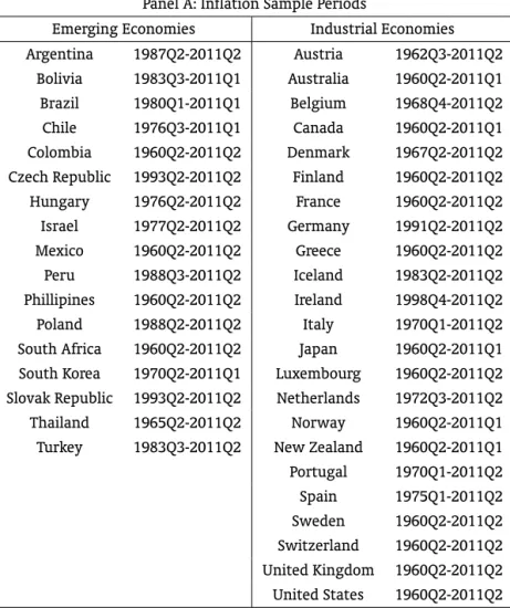
Table 1 Panel A shows the sample periods for the inflation series of all countries we analyze. For several of them, the sample period starts at the second quarter of 1960. The countries in which the samples periods are lower are Czech Republic and Slovak Republic, in which the data starts at the second quarter of 1993.

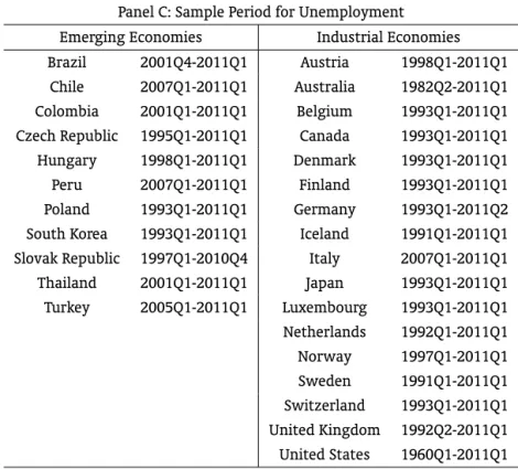
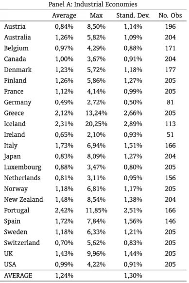
Table 1 Panel B shows the sample periods for the GDP of all countries in our sample. For most countries, the series of GDP are much smaller than the series of inflation. In the case of unemployment, as Table 1 Panel C shows the sample are even much shorter than both the samples of inflation and GDP for almost all countries except for the United States, where the series starts in the first quarter of 1960. In Table 2, we present descriptive statistics of the inflation processes. Table 2 Panel A shows that average quarterly inflation in industrial economies is 1.24% and that the average standard deviation is 1.30%. The country with the highest average inflation is Portugal, 2.42%, and with the highest standard deviation is Iceland with 2.89%.

Table 2 Panel B shows descriptive statistics of inflation for the group of emerging economies that did not have hyperinflation episode in the last thirty years. One can see that average inflation is 2.08% and average standard deviation is 2.07%. The economy with the highest average inflation is Colombia, 3.67%, and with the highest standard deviation is Hungary, 2.85%.

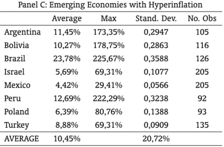
Table 2 Panel C shows descriptive statistics of inflation for the group of emerging economies that experienced a hyperinflation episode in the last thirty years. We can see that average inflation is 10.45% and average standard deviation is 20.72%. The economy with the highest average inflation and standard deviation is Brazil, 23.78%, and 35.88% respectively.

(5)

3. EMPIRICAL ANALYSIS

There is little agreement in the literature on how to measure inflation persistence. Therefore, we examine a set of econometric methods that attempt to capture the persistence in inflation. The results reported in this section are based on some of the methods that are most frequently used in the literature. They range from unit root tests in the presence of unknown structural breaks to the estimation of reduced-form models of inflation dynamics.

3.1. Unit root tests

As it is well known, a process that has a unit root is a highly persistent one. To verify if any of our inflation processes has a unit root and structural breaks, we follow two steps. In the first step, we test for the presence of a unit root with Aumengted Dick Fueller (1979), ADF, and for the presence

of structural breaks with Quandt-Andrews and Andrews e Ploberger (1994).14 _{Only in the case of the}

inflation processes of Germany and Austria, we reject the null of a unit root as well as the presence of

structural breaks.15

In the second step, following Kim e Perron (2009) we test for the presence of a unit root in the presence of unknown structural breaks for all inflation processes with the exception of Germany and Austria. Kim and Perron allow for the possibility of an unknown structural break both for the Hypotheses of a unit root process, the null Hypotheses, as well as for the Hypotheses of stationary process, the alternative Hypotheses. In all our tests, we consider the possibility of an unknown

structural break both at the intercept and at the trend.16

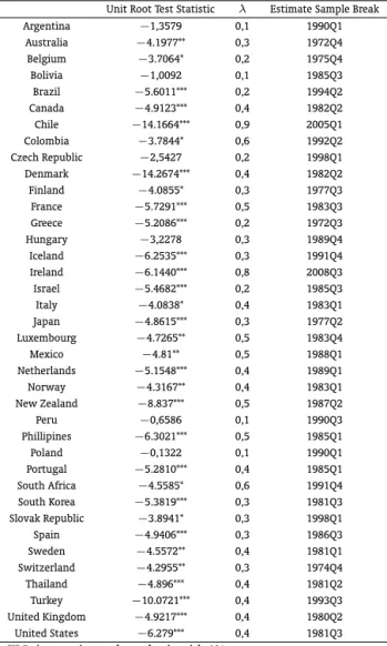
Table 3 presents the results. In the case of some emerging economies – Argentina, Peru, Bolivia, Hungary and Czech Republic – we accept the null hypothesis of a unit root in the presence of unknown structural breaks. Of these countries, three have experienced hyperinflation in the recent past. For all other inflation processes, we reject the null.

3.2. Autoregressive processes

After the unit root tests, we estimate reduced form specifications. We will explore several

possibilities. They range from autoregressive dynamics to different specifications of new Keynesian Phillips curves.

One of the most obvious ways of measuring inflation persistence is to regress inflation on its first lag as in equation (1) below. The estimated coefficient of the first lag of inflation is the first order autocorrelation coefficient of the inflation series.

πt=β0+β1πt−1+εt,E[εt] = 0,V ar(εt) =σ 2

ε (1)

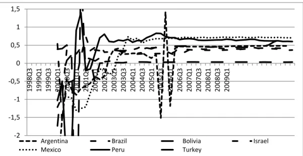
Figure 1 to 3 presents rolling samples estimates with a ten year window of theses coefficients for industrial, emerging economies without hyperinflation and emerging economies with hyperinflation

respectively.17

14_{We use the trimmings 10%, 15%, 25% and 35% for the Quandt-Andrews and Andrews-Ploberg tests and equation (2) in the text} without the dummies representing structural breaks as our specifications .

15_{In the case of Austria, the}_p_{-value of the ADF test is 0.083 and in the case of Germany the}_p_{-value of the ADF is 0.00.} 16_{The possibility of existence of more than one break was also considered for some countries, like Argentina for example. In this}

case, we used Kim e Perron (2009) with rolling samples. We continue to reject and not the unit root for the same countries as is shown in Table 3.

(6)

In Figure 1, we present the estimated coefficients for some industrial countries. As one can see,

inflation persistence is decreasing overt time for these countries.18_{In the case of emerging economies,}

we see a mixed result from Figures 2 and 3. In the case of emerging without hyperinflation, Slovak Republic, for instance, presents increasing persistence. Some emerging with hyperinflation, such as Brazil and Peru for example, present decreasing persistence while others like Bolivia, Turkey and Mexico show increasing persistence.

Another form of measuring inflation persistence is by regressing inflation on several of its lags as in equation (2) and then calculating the sum of coefficients on lagged inflation. If the sum of coefficients is close to 1 in a statistical sense, then shocks to inflation have long lived effects on inflation. The higher the sum of the coefficients of inflation lags, the longer it takes for inflation to return back to its mean, or the more persistent is the inflationary process.

πt=β0+β1πt−1+

L

X

k=1

φkπt−k+εt,E[εt] = 0,V ar(εt) =σ 2

ε (2)

whereπtis headline consumer inflation.

To the extent that lagged inflation captures true persistence in the price setting process the model implies that rapid reductions of inflation can only be produced at the cost of substantial increase in unemployment or decrease in product. Hence, the model points to a gradualist approach as providing the best way to effect a large reduction in inflation.

An equivalent approach for analyzing persistence (and the one we will follow in this paper) is to

estimateρin equation (3) as?show.

πt = β0+

D

X

j=1

dj+ρπt₋1+

D

X

j=1

ρdjπt−1+

L

X

k=1

△πt₋k+εt

E[εt] = 0,V ar(εt) =σ2

ε (3)

There are a number of good reasons for focusing onρas our main measure of inflation persistence.

For example, in this model,ρis a crucial determinant of the response to shocks over time. It can also

be shown that1/(1−ρ)gives the infinite-horizon cumulative impulse response to shocks.

In equation (3), we also use as regressors, so as to indicate structural breaks, dummies alone and

dummies interacting with the first lag of the inflation process.19 The dummies for most countries are

related to structural breaks that we observe using Quandt-Andrews and Andrews e Ploberger (1994)

with rolling samples.20 _{For some, we obtain the same structural breakpoints as in Kim e Perron (2009)}

unit root tests. Table 4 presents the quarters in which we consider a structural break for all countries, with the exception of Germany and Austria, in our sample period.

We choose the number of lags of first difference of headline consumer inflation in (3) so as the

residuals do not present serial correlation, using Breusch-Godfrey LM test to identify serial correlation.21

We also check for heteroskedasticity with ? and Breusch e Pagan (1979). If there is evidence of

heteroskedasticity, we correct it with the Newey e West (1987) robust errors. We do a Wald test for the sum of persistence coefficients equal to one for all estimations.

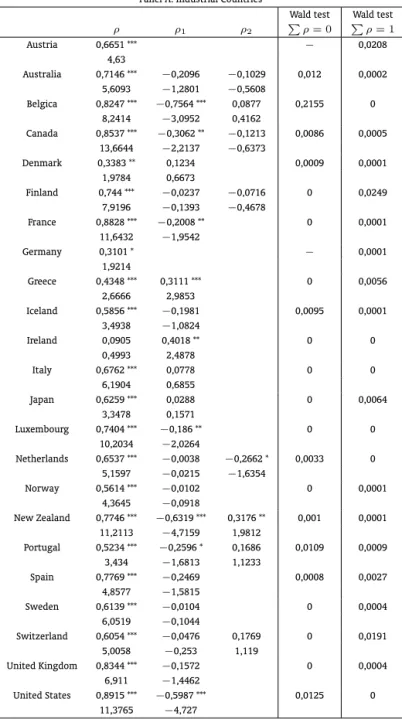
Table 5 Panel A shows the estimated persistence coefficients for this specification for industrial economies including the dummies of structural breaks. The majority of industrial countries (78%) show

18_{This is what happens for most industrial economies. For the others industrial sthat are not in Figure 1, the estimated} coefficients are available upon request to the authors.

19_{Dummies are represented by}_d_and_D_{is the total number of dummies.}

(7)

decreasing persistence over time, as one can see.22 _{For all industrial countries, we reject the null}

hyphoteses of sum of the persistence coefficients equal to one.

Tabel 5 Panel B shows the estimation of equation (3) for emerging economies. As one can see, some countries like Chile, Israel, Mexico, Poland, Turkey and Slovak Republic show increasing persistence. Of these, Turkey and Poland are hyperinflation countries. The other hyperinflation countries show decreasing persistence. This is the case of Brazil for instance. Once more, we reject the null hypotheses of sum of the persistence coefficients equal to one.

We repeat the estimation above including in equation (2) the output gap calculated using Hodrick-Prescot filter. Again, we test for serial correlation, heteroskedasticity, and in their presence we correct using Newey-West.

The results for the industrial economies are very similar to the ones described above (see Table 6 Panel A). However for emerging economies, the results differ somewhat from the previous ones. No emerging economy presents increasing persistence.

We think that this result has may be related to two distinct explanations. The first is that inflation persistence for these countries could be associated with changes in its intrinsic driving process, rather than solely changes in its dynamics. Several of these emerging market economies in the recent years have implemented more aggressive monetary policy and this could have had an effect over GDP gap and thus in inflation persistence. The second explanation may be related to the fact that our series of GDP for each country is shorter than the series of inflation for most countries in our sample, particularly for emerging ones.

We will estimate in the following section new Keynesian models of inflation that incorporate

inflation expectations. This will allow us to capture if monetary policy has anchored inflation

expectations more solidly in the last years. This could have important implications to inflation

persistence,

3.3. New Keynesian Phillips curves estimation

The most important implication of the pure new Keynesian model of inflation is that there is no intrinsic persistence in inflation in the sense that there is no structural dependence of inflation on its own lagged values. Instead, inflation is determined in a completely forward-looking manner. One implication of this model in contrast to traditional ones is that it is much easier to quickly reduce inflation in this model than in the traditional one. In fact, according to the new Keynesian model,

inflation can be costless controlled by a credible commitment to keep output close to its potential.23

Due to the difficulty of fitting the data with new Keynesian pure forward-looking model, a vast

literature that incorporates lags of inflation in the new Keynesian Phillips curve (NKPC) has emerged.24

For many, this class of models represents a sort of common-sense middle ground that preserves the insights of standard rational expectations models while allowing for better empirical fit by dealing directly with a well known deficiency of the pure forward looking model of inflation. As a result this class of models has been widely used in applied monetary policy analysis.

The structural equation for inflation that we estimate is in the spirit of hybrid new Keynesian Phillips curve as in (3). These models add a dependence of inflation on its lagged values to otherwise

22_{This can be observed by the looking at the sum of the persistent coefficients alone and interacting with dummies of structural} breaks.

23_{The most popular formulation of the new Keynesian framework is based on Calvo (1983) model of price random adjustment.} The model assumes that in each period a random fraction of firms reset their price while all other firms keep their prices unchanged. Calvo assumes an imperfectly competitive market structure as well. These two hypotheses generate the basic new Keynesian model of inflation.

(8)

purely forward looking models. Such models are often considered as a compromise between the need for rigorous micro foundations of the sort underlying the pure new-Keynesian Phillips curve and the need to fit the data empirically.

πt = D

X

j=1

dj+ρπt₋1+

D

X

j=1

ρdjπt−1+ (1−ρ)Et[πt+1]

+ β2ht−1+εt,E[εt] = 0,var(εt) =σ 2

ε (4)

wherehtis output gap.

The parameter that measures inflation persistence isρ. Again, we interact this parameter with

dummies indicating structural breaks (dare the dummies andDis the total number of dummies).

We use two different instruments for the expectation of inflation one period ahead. One instrument

are lags of current inflation.25 The other instrument are forecasts of inflation obtained from a VAR with

inflation and GDP gap as dependent variables. In this case, the number of lags of the VAR is chosen using Akaike information criteria.

We also check for serial correlation with Breusch-Godfrey LM test and for heteroskedasticity with

? test. In the presence of serial correlation, we include more lags of regressors, until there is no more

evidence of serial correlation. In the presence of heteroskedasticity, we correct with Newey-West (1987) robust matrix.

Table 7 Panels A and B shows the estimated persistence with the lags of current inflation as

instruments for industrial and emerging economies respectively. Table 7 Panels C and D shows

the estimated persistence with the forecast of inflation of the inflation equation of the VAR as an instrument.

The results for estimations with both instruments are somewhat different from the ones we find before. Several industrial economies have the sum of the persistent coefficient not statistically significant. For those that are significant, we observe a decrease in persistence. In the case of emerging economies, the results are mixed. Some of these countries show significant and increasing persistence while others have decreasing persistence. Again, we think that these results may be associated with changes in its intrinsic driving process of inflation and with the fact that we have very different sample periods of GDP data for all countries, particularly for emerging ones.

3.4. Robustness tests

We include wage rigidity in the new Keynesian framework in line with Gali e Blanchard (2005). The objective is to see if there is a change in estimated persistence due to these rigidities.

Gali e Blanchard (2005) incorporate wage rigidities in the structural model of inflation. One

implication of Gali e Blanchard (2005) model is the relation between inflation and unemployment as

in equation (4). Theρcoefficient continues to measure inflation persistence. Gali and Blanchard show

that this coefficient is an increasing function of wage rigidity.

πt = D

X

j=1

dj+ρπt₋1+

D

X

j=1

ρdjπt−1+ (1−ρ)Et[πt+1] +β1ut−1+εt

E[εt] = 0,var(εt) =σ2

ε (5)

(9)

As Mishkin (2007) points out, when researchers estimate this equation they typically find that the coefficient on the unemployment gap has declined in the absolute value since the 1980s often by a marked amount. In other words, the evidence suggests that the Phillips curve has flattened.

Table 8 Panels A and B shows the estimated ρfor this specification. Due to the limitations of

unemployment data in our sample, we cannot use as regressors dummies of structural breaks for almost all countries. So it is not appropriate to say anything about increasing or decreasing persistence for this empirical analysis. However, one can observe that several industrial countries present negative and significant coefficients (very low persistence) while most emerging economies present significant and over 0.40 coefficient of persistence. The highest significant coefficient for industrial countries is 0.3983, while for emerging is 0.67652 (Mexico) that is a hyperinflation country.

We also perform several other robustness tests. We look at the inflation correlograms, decompose all inflation series in trend and cycle and do some recursive least squares (recursive coefficients) analyses for the whole sample and for subsamples of the data of each country. Due to space restrictions, we do

not report the results.26 _{All these analyses, in general terms, confirm the main empirical evidences we}

present above in this paper.

3.5. Discussion of the results

After gauging all the empirical evidence that we find- considering several unit root tests with unknown structural breaks, the estimation of reduced form inflation dynamics and various robustness tests- we ponder that, in general terms, our results indicate that most industrial economies experience decreasing inflation persistence over time, while in the case of emerging economies several show increasing and even some present highly persistent inflationary processes. Of the former group, some are countries that experienced hyperinflation in the recent past.

In interpreting our results, we must first recognize that all of them are based on reduced-form relationships. Thus, they are about correlations and not necessarily about true structural relationships. Explanatory variables in our inflation estimations are themselves influenced by changes in economic conditions. So, changes in the underlying monetary policy regime are likely to be a source changes in reduced-form inflation dynamics. This problem is especially acute for structural relationship involving expectations or other factors that are not directly observable and so cannot be included in reduced form regressions. In such cases, we cannot use the reduced form equations to disentangle the effects of such unobserved factors which themselves may be driven by changes in monetary policy from that of other influences.

In terms of macroeconomic policies, we think that these results are important for emerging economies. Despite some recent improvements in these policies in some of these countries, inflation persistence is still an important issue for them. Due to the fact that inflation persistence increases the cost of disinflation, emerging economies should focus on macroeconomic policies, particularly monetary policies, to decrease this persistence in the near future.

4. CONCLUSION

We analyze inflation persistence in several industrial and emerging countries in the recent past by implementing unit root tests in the presence of unknown structural breaks and by estimating reduced-form models of inflation dynamics. We select a very representative group of 23 industrial and 17 emerging economies.

Our results show that inflation persistence is mostly decreasing over time for the industrial economies. Many emerging economies, however, show increasing persistence over time and even some have very persistent inflationary processes. We also find that the great majority of inflationary

(10)

processes present structural breaks in their sample periods, which indicate that they have not been stable.

Mishkin (2007) makes it clear that inflation expectations must be a key driving force behind inflation. This dependence has long been implicit in traditional Phillips curve analysis but now expectations are explicit and are also a central feature of new Keynesian Phillips curves in which current period inflation is a function of expectations next period and output gap.

Anchoring of inflation expectations must be related to monetary policy. During the past years several central banks have increased their commitment to price stability in both words and action. The Federal Reserve, the European Central Bank and other central banks of industrial and some of emerging economies have been committed to keep inflation under control.

For many emerging economies, however, our empirical evidence indicates that anchoring inflation expectations is problematic still because of high inflation persistence that we observe. The increase of monetary policy effectiveness in these countries thus is related to the capacity their central banks will have to decrease inflation persistence in the next years.

BIBLIOGRAPHY

Altissimo, F., Ehrmann, M., & Smets, F. (2006). Inflation persistence and price-setting behavior in the Euro area. A summary of the IPN evidence. Occasional Paper Series 46, European Central Bank.

Andrews, D. W. K. (1993). Tests for parameter instability and structural change with unknown change

point. Econometrica, 62:1383–1414.

Andrews, D. W. K. & Ploberger, W. (1994). Optimal tests when a nuisance parameter is present only

under the alternative.Econometrica, 62:1383–1414.

Batini, N. (2002). Euro area inflation persistence. Working Paper 201, ECB.

Benati, L. (2008). Investigating inflation persistence across monetary regimes. Quarterly Journal of

Economics, 123:1005–1060.

Breusch, T. S. (1979). Testing for autocorrelation in dynamic linear models. Australian Economic Papers,

17:334–355.

Breusch, T. S. & Pagan, A. R. (1979). Simple test for heteroscedasticity and random coefficient variation.

Econometrica, 47:1287–1294.

Calvo, G. (1983). Staggered prices in a utility maximizing framework. Journal of Monetary Economics,

12:383–398.

Cechetti, G. S., Hooper, P., Kasman, C. B., Schoenholtz, L. K., & Watson, W. M. (2007). Understanding the

evolving inflation process. In University, B., editor,U.S. Monetary Policy Forum.

Dickey, D. A. & Fuller, W. A. (1979). Distribution of the estimators for autoregressive time series with a

unit root. Journal of the American Statistical Association, 74:427–431.

Dossche, M. & Everaert, G. (2005). Measuring inflation persistence. A structural time series approach. Working Paper 495, ECB.

Fuhrer, C. J. (2005). Intrinsic and inherited inflation persistence. Working Paper Series 05, Federal Reserve Bank of Boston.

(11)

Fuhrer, C. J. & Moore, G. (1995). Inflation persistence. Quartely Journal of Economics, 110:127–159.

Gali, J. & Blanchard, O. (2005). Real wage rigidities and the new keynesian model. In Conference on

Quantitative Evidence of Price Determination, pages 29–30, Washington D.C.

Gali, J. & Gertler, M. (1999). A structural econometric analysis. Journal of Monetary Economics,

44:195–222.

Godfrey, L. G. (1978). Testing against general autoregressive and moving average error models when

the regressors include lagged dependent variables. Econometrica, 46:1293–1302.

Kim, D. & Perron, P. (2009). Unit root tests allowing for a break in the trend function at an unknown

time under both the null and alternative hypotheses. Journal of Econometrics, 148:1–13.

L., C., Einchenbaum, M., & Charles, E. (2005). Nominal rigidities and the dynamics effects of shocks to

monetary policy. Journal of Political Economy, 113:1–45.

Mishkin, S. F. (2007). Inflation dynamics. Working Paper Series National Bureau of Economic Research 13147, NBER.

Nason, M. J. (2006). Instability in U.S. inflation:1967-2005. Working paper, Federal Reserve Bank of Atlanta.

Newey, W. K. & West, K. D. (1987). A simple, positive semi-definite, heteroskedasticity and

autocorrelation consistent covariance matrix. Econometrica, 55:703–708.

Quandt, R. (1960). Tests of the hypothesis that a linear regression obeys two separate regimes. Journal

of the American Statistical Association, 55:324–330.

Rudd, J. & Whelan, K. (2005). Modelling inflation dynamics: A critical review of recent research. working paper series, Federal Reserve Board.

Stock, H. J. & Watson, W. M. (2006). Why has U.S. inflation become harder to forecast? Working Paper Series National Bureau of Economic Research 12324, NBER.

Taylor, J. (1999). Staggered price and wage setting in macroeconomic. In Taylor & Woodford, editors,

(12)

Table 1: Sample Periods

Our data are quarterly and differs depending on the country. We select 40 countries: 23 industrial and 17 emerging. Our data source is the International Financial Statistics of the International Monetary Fund. Our measure of inflation is headline Consumer Price Index inflation, CPI. We use as exogenous the following variables: the GDP gap, which is the difference between nominal GDP and potential GDP obtained through Hodrick-Prescott filtering and the unemployment rate. Panel A presents the sample periods for inflation. Panel B presents the sample periods for GDP and Panel C shows the sample periods for unemployment.

Panel A: Inflation Sample Periods

Emerging Economies Industrial Economies

Argentina 1987Q2-2011Q2 Austria 1962Q3-2011Q2

Bolivia 1983Q3-2011Q1 Australia 1960Q2-2011Q1

Brazil 1980Q1-2011Q1 Belgium 1968Q4-2011Q2

Chile 1976Q3-2011Q1 Canada 1960Q2-2011Q1

Colombia 1960Q2-2011Q2 Denmark 1967Q2-2011Q2

Czech Republic 1993Q2-2011Q2 Finland 1960Q2-2011Q2

Hungary 1976Q2-2011Q2 France 1960Q2-2011Q2

Israel 1977Q2-2011Q2 Germany 1991Q2-2011Q2

Mexico 1960Q2-2011Q2 Greece 1960Q2-2011Q2

Peru 1988Q3-2011Q2 Iceland 1983Q2-2011Q2

Phillipines 1960Q2-2011Q2 Ireland 1998Q4-2011Q2

Poland 1988Q2-2011Q2 Italy 1970Q1-2011Q2

South Africa 1960Q2-2011Q2 Japan 1960Q2-2011Q1

South Korea 1970Q2-2011Q1 Luxembourg 1960Q2-2011Q2

Slovak Republic 1993Q2-2011Q2 Netherlands 1972Q3-2011Q2

Thailand 1965Q2-2011Q2 Norway 1960Q2-2011Q1

Turkey 1983Q3-2011Q2 New Zealand 1960Q2-2011Q1

Portugal 1970Q1-2011Q2

Spain 1975Q1-2011Q2

Sweden 1960Q2-2011Q2

Switzerland 1960Q2-2011Q2

United Kingdom 1960Q2-2011Q2

(13)

Table 1 – Sample Periods

Panel B: Sample Period for GDP

Argentina 1993Q1-2010Q4 Austria 1964Q1-2010Q4

Bolivia 1995Q1-2009Q3 Australia 1960Q1-2010Q4

Brazil 1993Q3-2010Q4 Belgium 1980Q1-2010Q4

Chile 1996Q1-2010Q4 Canada 1960Q1-2010Q4

Colombia 1990Q1-2010Q4 Denmark 1977Q1-2010Q4

Czech Republic 1990Q1-2010Q4 Finland 1970Q1-2010Q4

Hungary 1995Q1-2010Q4 France 1965Q1-2010Q4

Israel 1971Q1-2010Q4 Germany 1960Q1-2010Q4

Mexico 1981Q1-2010Q4 Greece 2000Q1-2010Q4

Peru 1979Q1-2010Q4 Iceland 1997Q1-2010Q4

Phillipines 1980Q4-2010Q4 Ireland 1997Q1-2010Q4

Poland 1995Q1-2010Q4 Italy 1960Q1-2010Q4

South Africa 1960Q1-2010Q4 Japan 1960Q1-2010Q4

South Korea 1960Q1-2010Q4 Luxembourg 1995Q1-2010Q4

Slovak Republic 1993Q1-2010Q4 Netherlands 1977Q1-2010Q4

Thailand 1993Q1-2010Q4 Norway 1961Q1-2010Q4

New Zealand 1987Q2-2010Q4

Portugal 1977Q1-2010Q4

Spain 1970Q1-2010Q4

(14)

Table 1 – Sample Periods

Panel C: Sample Period for Unemployment

Brazil 2001Q4-2011Q1 Austria 1998Q1-2011Q1

Chile 2007Q1-2011Q1 Australia 1982Q2-2011Q1

Colombia 2001Q1-2011Q1 Belgium 1993Q1-2011Q1

Czech Republic 1995Q1-2011Q1 Canada 1993Q1-2011Q1

Hungary 1998Q1-2011Q1 Denmark 1993Q1-2011Q1

Peru 2007Q1-2011Q1 Finland 1993Q1-2011Q1

Poland 1993Q1-2011Q1 Germany 1993Q1-2011Q2

South Korea 1993Q1-2011Q1 Iceland 1991Q1-2011Q1

Slovak Republic 1997Q1-2010Q4 Italy 2007Q1-2011Q1

Thailand 2001Q1-2011Q1 Japan 1993Q1-2011Q1

Turkey 2005Q1-2011Q1 Luxembourg 1993Q1-2011Q1

Netherlands 1992Q1-2011Q1

Norway 1997Q1-2011Q1

(15)

Table 2: Descriptive Statistics of Inflation

Our data are quarterly and differs depending on the country. We select 40 countries: 23 industrial and 17 emerging. Our data source is the International Financial Statistics of the International Monetary Fund. Our measure of inflation is headline Consumer Price Index inflation, CPI. Panel A presents the descriptive statistics of inflation for industrial economies. Panel B presents the descriptive statistics for emerging economies that did not have hyperinflation. Panel C presents the descriptive statistics of inflation of countries that experienced hyperinflation in the recent past according to our criteria.

Panel A: Industrial Economies

Average Max Stand. Dev. No. Obs

Austria 0,84% 8,50% 1,14% 196

Australia 1,26% 5,82% 1,09% 204

Belgium 0,97% 4,29% 0,88% 171

Canada 1,00% 3,67% 0,91% 204

Denmark 1,23% 5,72% 1,18% 177

Finland 1,26% 5,86% 1,27% 205

France 1,12% 4,14% 0,99% 205

Germany 0,49% 2,72% 0,50% 81

Greece 2,12% 13,24% 2,66% 205

Iceland 2,31% 20,25% 2,89% 113

Ireland 0,65% 2,10% 0,93% 51

Italy 1,73% 6,94% 1,51% 166

Japan 0,83% 8,09% 1,27% 204

Luxembourg 0,88% 3,47% 0,80% 205

Netherlands 0,81% 3,11% 0,95% 156

Norway 1,18% 6,81% 1,17% 205

New Zealand 1,48% 8,54% 1,38% 204

Portugal 2,42% 11,85% 2,51% 166

Spain 1,72% 7,84% 1,56% 146

Sweden 1,18% 6,33% 1,21% 205

Switzerland 0,70% 5,62% 0,83% 205

UK 1,43% 9,96% 1,44% 205

USA 0,99% 4,22% 0,91% 205

(16)

Table 2 – Descriptive Statistics of Inflation

Panel B: Emerging Economies without Hyperinflation

Chile 2,57% 10,37% 0,0237 120

Colombia 3,67% 14,39% 0,0282 205

Czech Republic 1,10% 4,72% 0,0118 73

Hungary 2,62% 15,82% 0,0285 141

Phillipines 2,21% 14,85% 0,0261 205

South Africa 2,01% 6,35% 0,014 205

South Korea 1,82% 13,03% 0,0217 164

Slovak Republic 1,53% 6,66% 0,0162 73

Thailand 1,20% 10,64% 0,0163 185

AVERAGE 2,08% 2,07%

Table 2 – Descriptive Statistics of Inflation

Panel C: Emerging Economies with Hyperinflation

Argentina 11,45% 173,35% 0,2947 105

Bolivia 10,27% 178,75% 0,2863 116

Brazil 23,78% 225,67% 0,3588 126

Israel 5,69% 69,31% 0,1077 205

Mexico 4,42% 29,41% 0,0566 205

Peru 12,69% 222,29% 0,3238 92

Poland 6,39% 80,76% 0,1388 93

Turkey 8,88% 69,31% 0,0909 135

(17)

Table 3: Unit Root Tests with Structural Breaks

Our data are quarterly and differs depending on the country. We select 40 countries: 23 industrial and 17 emerging. Our data source is the International Financial Statistics of the International Monetary Fund. Our measure of inflation is headline Consumer Price Index inflation, CPI. The unit root test with unknown breaks both at the null at the alternative hyphoteses is based on Kim e Perron (2009).

Unit Root Test Statistic λ Estimate Sample Break Argentina −1,3579 0,1 1990Q1

Australia −4.1977** 0,3 1972Q4 Belgium −3.7064* 0,2 1975Q4 Bolivia −1,0092 0,1 1985Q3 Brazil −5.6011*** 0,2 1994Q2 Canada −4.9123*** 0,4 1982Q2 Chile −14.1664*** 0,9 2005Q1 Colombia −3.7844* 0,6 1992Q2 Czech Republic −2,5427 0,2 1998Q1 Denmark −14.2674*** 0,4 1982Q2 Finland −4.0855* 0,3 1977Q3 France −5.7291*** 0,5 1983Q3 Greece −5.2086*** 0,2 1972Q3 Hungary −3,2278 0,3 1989Q4 Iceland −6.2535*** 0,3 1991Q4 Ireland −6.1440*** 0,8 2008Q3 Israel −5.4682*** 0,2 1985Q3 Italy −4.0838* 0,4 1983Q1 Japan −4.8615*** 0,3 1977Q2 Luxembourg −4.7265** 0,5 1983Q4 Mexico −4.81** 0,5 1988Q1 Netherlands −5.1548*** 0,4 1989Q1 Norway −4.3167** 0,4 1983Q1 New Zealand −8.837*** 0,5 1987Q2

Peru −0,6586 0,1 1990Q3

Phillipines −6.3021*** 0,5 1985Q1 Poland −0,1322 0,1 1990Q1 Portugal −5.2810*** 0,4 1985Q1 South Africa −4.5585* 0,6 1991Q4 South Korea −5.3819*** 0,3 1981Q3 Slovak Republic −3.8941* 0,3 1998Q1 Spain −4.9406*** 0,3 1986Q3 Sweden −4.5572** 0,4 1981Q1 Switzerland −4.2955** 0,3 1974Q4 Thailand −4.896*** 0,4 1981Q2 Turkey −10.0721*** 0,4 1993Q3 United Kingdom −4.9217*** 0,4 1980Q2 United States −6.279*** 0,4 1981Q3 *** Rejects unit root hypothesis with 1%.

(18)

Figure 1: Estimated Autocorrelation Coefficients: Industrial Economies

-6 -5 -4 -3 -2 -1 0 1 2 3 4

19

99Q1

19

99Q3

20

00

Q1

20

00Q3

20

01Q1

20

01Q3

20

02Q1

20

02Q3

20

03Q1

20

03Q3

20

04Q1

20

04Q3

20

05

Q1

20

05Q3

20

06Q1

20

06Q3

20

07Q1

20

07Q3

20

08Q1

20

08Q3

20

09Q1

Australia Canada Iceland Norway

Sweden Austria Belgium Denmark

Finland France Greece Ireland

(19)

Figure 2: Estimated Autocorrelation Coefficients: Emerging Economies without Hyperinflation -3.5 -2.5 -1.5 -0.5 0.5 1.5 1 9 9 8 Q 3 1 9 9 9 Q 1 1 9 9 9 Q 3 2 0 0 0 Q 1 2 0 0 0 Q 3 2 0 0 1 Q 1 2 0 0 1 Q 3 2 0 0 2 Q 1 2 0 0 2 Q 3 2 0 0 3 Q 1 2 0 0 3 Q 3 2 0 0 4 Q 1 2 0 0 4 Q 3 2 0 0 5 Q 1 2 0 0 5 Q 3 2 0 0 6 Q 1 2 0 0 6 Q 3 2 0 0 7 Q 1 2 0 0 7 Q 3 2 0 0 8 Q 1 2 0 0 8 Q 3 2 0 0 9 Q 1

Chile Colombia Czech Rep.

Hungary Korea Phillipines

South Africa Thailand Slovak Rep.

Figure 3: Estimated Autocorrelation Coefficients: Emerging Economies with Hyperinflation

-2 -1,5 -1 -0,5 0 0,5 1 1,5 19 98 Q3 19 99Q1 19 99Q3 20 00Q1 20 00Q3 20 01Q1 20 01Q3 20 02Q1 20 02Q3 20 03Q1 20 03Q3 20 04Q1 20 04Q3 20 05Q1 20 05Q3 20 06Q1 20 06Q3 20 07 Q1 20 07Q3 20 08Q1 20 08Q3 20 09Q1

Argentina Brazil Bolivia Israel

(20)

Table 4: Structural Breaks of Inflation for Reduced-Form Estimations

Our data are quarterly and differs depending on the country. We select 40 countries: 23 industrial and 17 emerging. Our data source is the International Financial Statistics of the International Monetary Fund. Our measure of inflation is headline Consumer Price Index inflation, CPI.

Argentina 1990Q1 Luxembourg 1983Q4

Australia 1972Q4 1990Q3 Mexico 1973Q4 1988Q1

Belgium 1975Q4 1984Q4 Netherlands 1982Q2 1989Q1

Bolivia 1986Q2 New Zealand 1987Q2 1990Q2

Brazil 1994Q2 Norway 1983Q1

Canada 1982Q2 1991Q1 Peru 1993Q2

Chile* 1992Q4 2005Q1 Phillipines 1985Q1

Colombia 1998Q1 Poland 1990Q1

Czech Republic 1998Q1 Portugal 1985Q1 1992Q1

Denmark 1982Q2 South Africa 1991Q4

Finland 1977Q3 1992Q4 South Korea 1981Q3

France * 1982Q2 Spain 1986Q3

Greece 1972Q3 Sweden 1990Q3 1978Q3

Hungary 1989Q4 Switzerland 1974Q4

Iceland 1991Q4 Thailand 1981Q2

Ireland 2008Q3 Turkey 2002Q4

Israel 1977Q3 United Kingdom 1980Q2

Italy 1983Q1 United States 1981Q3

(21)

Table 5: Autoregressive Processes of Inflation without Output Gap

Our data are quarterly and differs depending on the country. We select 40 countries: 23 industrial and 17 emerging. Our data source is the International Financial Statistics of the International Monetary Fund. Our measure of inflation is headline Consumer Price Index inflation, CPI. Panel A presents the results of the estimation of equation (2) in the text for industrial economies. Panel B presents the results of the estimation of equation (2) in the text for emerging economies. Below the estimated persistent coefficients in columns 1 to 3 of both panels A and B, we have at

statistic. In the last 2 columns of both Panels A and B, we havep-values.

Panel A: Industrial Countries

Wald test Wald test

ρ ρ₁ ρ₂ Pρ= 0 Pρ= 1 Austria 0,6651 *** − 0,0208

4,63

Australia 0,7146 *** −0,2096 −0,1029 0,012 0,0002 5,6093 −1,2801 −0,5608

Belgica 0,8247 *** −0,7564 *** 0,0877 0,2155 0 8,2414 −3,0952 0,4162

Canada 0,8537 *** −0,3062 ** −0,1213 0,0086 0,0005 13,6644 −2,2137 −0,6373

Denmark 0,3383 ** 0,1234 0,0009 0,0001 1,9784 0,6673

Finland 0,744 *** −0,0237 −0,0716 0 0,0249 7,9196 −0,1393 −0,4678

France 0,8828 *** −0,2008 ** 0 0,0001 11,6432 −1,9542

Germany 0,3101 * − 0,0001 1,9214

Greece 0,4348 *** 0,3111 *** 0 0,0056 2,6666 2,9853

Iceland 0,5856 *** −0,1981 0,0095 0,0001 3,4938 −1,0824

Ireland 0,0905 0,4018 ** 0 0 0,4993 2,4878

Italy 0,6762 *** 0,0778 0 0 6,1904 0,6855

Japan 0,6259 *** 0,0288 0 0,0064 3,3478 0,1571

Luxembourg 0,7404 *** −0,186 ** 0 0 10,2034 −2,0264

Netherlands 0,6537 *** −0,0038 −0,2662 * 0,0033 0 5,1597 −0,0215 −1,6354

Norway 0,5614 *** −0,0102 0 0,0001 4,3645 −0,0918

New Zealand 0,7746 *** −0,6319 *** 0,3176 ** 0,001 0,0001 11,2113 −4,7159 1,9812

Portugal 0,5234 *** −0,2596 * 0,1686 0,0109 0,0009 3,434 −1,6813 1,1233

Spain 0,7769 *** −0,2469 0,0008 0,0027 4,8577 −1,5815

Sweden 0,6139 *** −0,0104 0 0,0004 6,0519 −0,1044

Switzerland 0,6054 *** −0,0476 0,1769 0 0,0191 5,0058 −0,253 1,119

United Kingdom 0,8344 *** −0,1572 0 0,0004 6,911 −1,4462

(22)

Table 5 – Autoregressive Processes of Inflation without Output Gap

Panel B: Emerging Economies

Wald test Wald test

ρ ρ1 ρ2 Pρ= 0 Pρ= 1

Argentina 1,0806 *** −0,7689 * 0,0332 0,0000

3,0575 −1,6467

Bolivia 0,1872 0,3675 0,4289 0,5251

0,9093 0,4165

Brazil 0,9341 *** −0,3997 ** 0,0050 0,0139

6,9822 −2,1925

Chile 0,2553 * 0,1962 −0,1212 0,0103 0,0000

1,7617 1,2358 −0,7874

Colombia 0,6088 *** −0,026 0,0000 0,0000

4,4359 −0,2221

Czech Republic 0,0462 0,3109 ** 0,0733 0,0017

0,2185 2,0067

Hungary 0,7207 *** 0,1815 * 0,0000 0,3261

5,2758 1,8061

Israel 0,0093 0,8217 *** −0,2759 ** 0,0000 0,0000

0,0886 7,5122 −2,2549

Mexico −0,3749 * 1,3488 *** −0,3454 *** 0,0000 0,0000

−1,7617 5,862 −3,2484

Peru 0,5656 ** 0,1445 0,0000 0,0000

2,1653 0,5513

Phillipines 0,5716 *** −0,1572 0,0009 0,0000

5,2584 −1,0167

Poland 0,1118 0,5466 *** 0,0000 0,0000

1,4007 5,5514

South Africa 0,8238 *** −0,0569 0,0000 0,0373

13,897 −0,4721

South Korea 0,2635 * −0,1381 0,2475 0,0000

1,7911 −0,9387

Slovak Republic 0,4791 ** 0,026 0,0142 0,0162

2,3529 0,2561

Thailand 0,6502 *** −0,3132 *** 0,0260 0,0000

4,5205 −2,6134

Turkey 0,1759 0,2728 0,0465 0,0149

0,9977 1,2168 *** Rejects with 1%.

** Rejects with 5%.

(23)

Table 6: Autoregressive Processes Estimation with Output Gap

Our data are quarterly and differs depending on the country. We select 40 countries: 23 industrial and 17 emerging. Our data source is the International Financial Statistics of the International Monetary Fund. Our measure of inflation is headline Consumer Price Index inflation, CPI. We use as exogenous the following variables: the GDP gap, which is the difference between nominal GDP and potential GDP obtained through Hodrick-Prescott filtering and the unemployment rate. Panel A presents the results of the estimation of equation (3) in the text for industrial economies with the inclusion of output gap. Panel B presents the results of the estimation of equation (3) in the text for emerging economies with the inclusion of output gap. Below the estimated persistent coefficients in columns 1 to 3 of both panels A and B, we have atstatistic. In the last 2 columns of both Panels A and B, we havep-values.

Panel A: Industrial Economies

Wald test Wald test

ρ ρ₁ ρ₂ Pρ= 0 Pρ= 1

Austria 0,6273 − −

5,2325

Australia 0,7152 −0,2097 −0,1027 0,013 0 3,6671 −1,0385 −0,6589

Belgium −0,4184 0,4828 0,656 0

−1,856 2,291

Canada 0,8641 −0,2993 −0,1119 0,005 0,028 11,12721 −1,455 −1,455

Denmark 0,4555 −0,0006 0,001 0 2,1673 −0,0033

Finland 0,5292 0,3147 0,0101 0 0,461 4,6721 2,1178 0,0501

France 0,8677 −0,1512 0 0 12,5946 −1,4931

Germany −0,1817 − −

−1,1145

Greece −0,2128 − −

−1,0395

Iceland 0,5504 − −

3,1813

Ireland 0,0578 0,4807 0,006 0,018 0,2299 1,6817

Italy 0,6979 0,1234 0 0,054 9,3732 1,0724

Japan 0,6425 0,0339 0 0,012 6,1977 0,251

Luxembourg −0,1121 − −

−0,5839

Netherlands 0,4482 0,1924 −0,3448 0,07 0 2,1914 0,8404 −1,8425

Norway 0,5626 −0,009 0 0,001 4,6979 −0,0654

New Zealand 0,3598 − − 3,4195

Portugal 0,2616 −0,285 0,2645 0,246 0 1,5215 −1,4687 1,0766

Spain 0,8001 −0,1872 0 0,01 7,0035 −1,274

Sweden 0,4444 0,1713 0 0,019 2,6728 1,1216

Switzerland 0,2082 0,3167 0,1265 0 0,009 1,0414 1,1405 0,5113

United Kingdom 0,7962 −0,043 0 0,017 10,3402 −0,3745

(24)

Table 6 – Autoregressive Processes Estimation with Output Gap

Panel B: Emerging Economies

Wald test Wald test

ρ ρ1 ρ2 Pρ= 0 Pρ= 1

Argentina 0,4069 4,6427

Bolivia 0,5894

3,9389

Brazil 0,2615

3,9715

Chile −0,2814 0,3313 0,7770 0,0000

−1,1696 1,3477

Colombia 0,8663 11,6388

Czech Republic 0,0720 0,3390 0,0930 0,0180

0,2005 1,0319

Hungary 0,8040

10,1117

Israel 0,7243 −0,1471 0,0000 0,0000

7,1765 −1,1697

Mexico 0,9996 −0,3453 0,0000 0,0000

7,7764 −2,5331

Peru −0,0867 0,8090 0,0000 0,0000

−0,3882 3,6291

Phillipines 0,7553 −0,3612 0,0020 0,0000

6,9186 −2,3982

Poland 0,6753

10,0075

South Africa 0,8204 −0,0582 0,0000 0,0570

11,2390 −0,4601

South Korea 0,2658 −0,1290 0,4000 0,0000

2,3163 −0,7722

Slovak Republic 0,5080 2,6988 Thailand −0,1628

(25)

Table 7: New Keynesian Phillips Curves Estimations

Our data are quarterly and differs depending on the country. We select 40 countries: 23 industrial and 17 emerging. Our data source is the International Financial Statistics of the International Monetary Fund. Our measure of inflation is headline Consumer Price Index inflation, CPI. We use as exogenous the following variables: the GDP gap, which is the difference between nominal GDP and potential GDP obtained through Hodrick-Prescott filtering and the unemployment rate. Panel A presents the results of the estimation of equation (4) in the text for industrial economies using the first lag of inflation as an instrument. Panel B presents the results of the estimation of equation (3) in the text for emerging economies using the first lag of inflation as an instrument. Panel C presents the results of the estimation of equation (3) in the text for industrial economies using as instrument the forecast of inflation from a VAR that has an inflation and GDP equation. Panel D presents the results of the estimation of equation (3) in the text for emerging economies using as instrument the forecast of inflation from a VAR that has an inflation and GDP equation. Below the estimated persistent coefficients in columns 1 to 3 of A, B, C and D we have atstatistic. In the last 2 columns of Panels A, B, C and D we havep-values.

Panel A: Lag Inflation as Instrument: Industrial Economies

Wald test Wald test

ρ ρ₁ ρ₂ Pρ= 0 Pρ= 1

Austria −0,4339 − −

−4,6312

Australia −0,1235 0,064 0,0341 0,858 0 −0,4122 0,2872 0,2069

Belgium −0,573 0,5019 0,514 0

−2,9873 2,4292

Canada 0,4773 −0,0308 −0,2964 0,222 0 2,2775 −0,1006 −1,2554

Denmark −0,0442 0,131 0,398 0

−0,2957 0,7686

Finland −1,0941 1,2501 0,1843 0,086 0,001 −5,0522 5,5031 0,7865

France 0,1404 0,0293 0,093 0 1,0302 0,271

Germany 0,1523 − −

1,5338

Greece 0,239 − −

2,04

Iceland −0,2396 − −

−0,9535

Ireland 0,0044 0,4623 0,015 0,006 0,0178 1,6863

Italy 0,2516 0,0722 0,004 0 2,3286 0,6957

Japan −0,1211 0,3261 0,073 0 −1,0094 2,1389

Luxembourg 0,1678 − −

1,3849

Netherlands 1,1656 −0,7432 −1,0346 0 0 4,9648 −2,6644 −4,051

Norway −0,2722 0,1755 0,415 0 −2,3894 1,1846

New Zealand 0,2645 − − 2,4981

Portugal 0,0606 0,2743 −0,6772 0,08 0 0,5638 1,2152 −2,524

Spain −0,4302 −0,8421 0 0 −2,3088 −6,4839

Sweden −0,9553 0,3054 0 0

−4,9944 1,7656

Switzerland −0,1635 0,2136 −0,1859 0,159 0

−1,1488 0,8173 −0,7157

United Kingdom −0,2333 0,4009 0,123 0 −1,5691 2,549

(26)

Table 7 – New Keynesian Phillips Curves Estimations

Panel B: Lag Inflation as Instrument: Emerging Economies

Wald test Wald test

ρ ρ1 ρ2 Pρ= 0 Pρ= 1

Argentina 0,5103 6,0301 Bolivia −0,0297

−0,1533

Brazil 0,3573

6,2320

Chile 0,1992 0,2894 0,0030 0,0002

1,2707 1,1668

Colombia 0,4556 3,9511

Czech Republic −0,6092 0,8990 0,0570 0,0000

−1,4706 1,8519

Hungary 0,5128

4,8017

Israel 0,6072 −0,1161 0,0000 0,0000

6,0488 −1,1051

Mexico 1,0311 −0,4072 0,0000 0,0000

6,8668 −3,1165

Peru 0,2638 0,0349 0,0003 0,0000

1,9529 0,4796

Phillipines 0,3751 0,1750 0,1030 0,0000

1,8733 −0,9015

Poland 0,5530

4,8120

South Africa −0,2424 0,1837 0,5960 0,0000

−1,5805 1,1693

South Korea −0,2230 −0,1205 0,0210 0,0000

−1,7879 −0,6821

Slovak Republic −0,1651

−1,1079

(27)

Panel C: Forecast of Inflation as Instrument: Industrial Economies Wald test Wald test

ρ ρ1 ρ2 Pρ= 0 Pρ= 1

Austria 0,1829 0,0620 0,0000

1,8785

Australia −0,0236 −0,0038 0,0280 0,9960 0,0000

−0,1938 −0,0337 0,1965

Belgium 0,1225 −0,1568 0,7510 0,0000

0,7326 −0,8402

Canada 0,2605 0,2050 −0,2445 0,0250 0,0000

2,6973 0,9707 −1,1834

Denmark −0,0111 0,1169 0,2790 0,0000

−0,0878 0,7762

Finland 0,2527 0,0544 −0,1556 0,5070 0,0000

2,0468 0,3083 −0,5844

France −0,1710 0,2049 0,5540 0,0000

−2,5696 3,3570

Germany 0,1655 0,0940 0,0000

1,6954

Greece 0,4628 0,0000 0,0000

4,4685

Iceland −0,7178 0,0000 0,0000

−4,0471

Ireland −0,1489 0,7137 0,0000 0,0000

−1,5899 5,1259

Italy 0,1481 0,1136 0,0030 0,0000

2,1255 1,3993

Japan −0,0985 0,3034 0,0380 0,0000

−1,1898 2,5273

Luxembourg −0,0916 0,4320 0,0000

−0,7909

Netherlands 1,3362 −0,8545 −0,9791 0,0000 0,0000

10,5396 −3,5587 −4,0437

Norway 0,1807 −0,1731 0,9530 0,0000

1,9646 −1,1714

New Zealand 0,0515 0,4630 0,0000

0,7379

Portugal 0,3446 −0,1238 −0,4643 0,2080 0,0000

2,7320 −0,5179 −1,7304

Spain 0,3125 −1,0829 0,0000 0,0000

1,9714 −8,0579

Sweden 0,2120 −0,4882 0,0740 0,0000

1,4413 −2,8604

Switzerland 0,3774 −0,1216 −0,2556 0,9980 0,0000

3,2650 −0,4223 −0,8752

United Kingdom 0,1440 0,0967 0,0150 0,0000

1,7883 0,8372

United States 0,5177 −0,4295 0,2860 0,0000

(28)

Panel D: Forecast of Inflation as Instrument: Emerging Economies Wald test Wald test

ρ ρ1 ρ2 Pρ= 0 Pρ= 1

Argentina 0,3915 0,0000 0,0000

7,0969

Bolivia 0,0153 0,8710 0,0000

0,1626

Brazil 0,3763 0,0000 0,0000

5,9203

Chile −0,0823 0,6751 0,0010 0,0016

−0,3927 2,1863

Colombia 0,4422 0,0000 0,0000

5,1762

Czech Republic −0,3430 0,5940 0,0690 0,0000

−1,4077 1,9632

Hungary 0,4562 0,0000 0,0000

4,9798

Israel −0,0313 0,4272 0,0000 0,0000

−0,3041 4,3904

Mexico 0,1588 0,2811 0,0000 0,0000

1,8271 3,5751

Peru 0,3118 0,0040 0,0000

2,9953

Phillipines 0,3207 −0,1447 0,0099 0,0000

3,1165 −1,1794

Poland 0,3736 0,0000 0,0000

4,6882

South Africa 0,0328 −0,0211 0,9090 0,0000

0,3517 −0,1728

South Korea −0,2532 −0,0877 0,0160 0,0000

−2,2912 −0,5362

Slovak Republic 0,1290 0,4240 0,0000

0,8044

Thailand −0,0680 0,5400 0,0000

(29)

Table 8: New Keynesian Phillips Curve with Wage Rigidities

Our data are quarterly and differs depending on the country. We select 40 countries: 23 industrial and 17 emerging. Our data source is the International Financial Statistics of the International Monetary Fund. Our measure of inflation is headline Consumer Price Index inflation, CPI. We use as exogenous the following variables: the GDP gap, which is the difference between nominal GDP and potential GDP obtained through Hodrick-Prescott filtering and the unemployment rate. Panel A presents the results of the estimation of equation (5) in the text for industrial economies using the first lag of inflation as an instrument. Panel B presents the results of the estimation of equation (4) in the text for emerging economies using the first lag of inflation as an instrument. Below the estimated persistent coefficients in columns 1 we have atstatistic. In the last columns of Panels A and B we havep-values.

Panel A: Industrial Economies Wald test

ρ ρ= 1 Austria −0,4439 0,0000

−4,7101

Australia −0,0386 0,0000

−0,3399

Belgium −0,1420 0,0000 −1,1263

Canada 0,2653 0,0000 2,3950

Denmark 0,0576 0,0000 0,4874

Finland −0,3080 0,0000 −2,3242

France 0,1333 0,0000 1,1797

Germany 0,1507 0,0000 1,4873

Greece 0,2346 0,0000 1,9177