Dissertação de Mestrado
Preference-guided Evolutionary
Algorithms for Optimization with Many
Objectives
Autor:
Fillipe Goulart
Orientador:
Dr. FelipeCampelo
Dissertação submetida à banca examinadora designada pelo Colegiado do
Programa de Pós-Graduação em Engenharia Elétrica da Universidade Federal de
Minas Gerais, como parte dos requisitos necessários para a obtenção do título de
Mestre em Engenharia
I, Fillipe Goulart, declare that this thesis, titled “Preference-guided Evolutionary
Al-gorithms for Optimization with Many Objectives”, and the work presented in it are my own. I confirm that:
This work was done wholly or mainly while in candidature for a research degree
at this University.
Where any part of this thesis has previously been submitted for a degree or any
other qualification at this University or any other institution, this has been clearly stated.
Where I have consulted the published work of others, this is always clearly
at-tributed.
Where I have quoted from the work of others, the source is always given. With
the exception of such quotations, this thesis is entirely my own work.
I have acknowledged all main sources of help.
Where the thesis is based on work done by myself jointly with others, I have made
clear exactly what was done by others and what I have contributed myself.
is not “Eureka!”, but “That’s funny”...
Abstract
Escola de Engenharia
Master of Engineering
Preference-guided Evolutionary Algorithms for Optimization with Many Objectives
by Fillipe Goulart
Resumo
I would like to thank my advisor for the patience and the guts for helping me with all the tough moments of this process of becoming a master, and for showing that there are still people in the world that use science for innovation, and not just for personal achievements.
I also want to thank Master Splinter, Old Master, Master System, Master Yoda, Master Roshi and all other masters that make this title worth all the hard work.
Last but not least, I want to thank my mother and my father for the support. I know that, even without understanding a single sentence of this text, they would still read it from cover to cover.
Declaration of Authorship i
Abstract vi
Acknowledgements viii
Contents ix
List of Figures xii
List of Tables xiv
1 Introduction 1
1.1 Scope of the problem. . . 2
1.2 Goals of This Dissertation . . . 2
1.3 Structure of the Work . . . 3
2 Multi-objective Optimization 4 2.1 Decision Making and Optimization . . . 5
2.2 Single-objective Optimization: When the Decision is Simple . . . 6
2.3 Multi-objective Optimization: Complicating the Decision Process . . . 8
2.3.1 Concept of efficiency, or Pareto-optimality . . . 11
2.3.1.1 Weak Efficiency . . . 14
2.3.1.2 Proper efficiency . . . 15
2.3.2 Boundaries of the Efficient front . . . 17
2.3.3 Shapes of the Efficient front . . . 19
2.3.4 Solving a Multi-objective Problem . . . 20
2.4 Methods for Finding Efficient Points . . . 22
2.4.1 Scalarizing methods . . . 23
2.4.1.1 Weighting Method . . . 24
2.4.1.2 ǫ-constraint Method . . . 27
2.4.1.3 Weighted Metrics . . . 29
2.4.1.4 Normal-boundary Intersection Method . . . 32
2.4.1.5 Review of Scalarizing Methods . . . 34
2.4.2 Deterministic Methods with no Scalarization . . . 35
2.4.2.1 Computing a Descent Direction . . . 36
2.4.2.2 Computing the step size. . . 39
2.4.2.3 The final algorithm . . . 41
2.4.3 Evolutionary Algorithms. . . 42
2.4.3.1 Non-dominated Sorting . . . 46
2.4.3.2 Indicator-based Evolutionary Algorithms . . . 49
2.4.3.3 Single-objective Differential Evolution . . . 52
2.4.3.4 Multi-objective Differential Evolution . . . 53
2.4.3.5 Review of Evolutionary Algorithms . . . 55
2.4.3.6 Interlude . . . 56
2.5 Summary . . . 56
3 Decision Making in Multi-objective Optimization 58 3.1 Decision Theory . . . 59
3.1.1 Basic concepts of Decision Theory . . . 59
3.1.1.1 Utility theory. . . 61
3.1.2 Solving a Decision Problem . . . 63
3.1.3 Choosing a solution in MOO . . . 64
3.2 Solution process in Multi-criteria Decision Making . . . 65
3.2.1 Classification of MOO methods . . . 65
3.2.1.1 A priori methods . . . 65
3.2.1.2 A posteriori methods . . . 66
3.2.1.3 Interactive methods . . . 67
3.2.1.4 Non-preference methods. . . 68
3.2.1.5 Other classifications . . . 68
3.2.2 Expressing the DM’s Preferences . . . 69
3.2.2.1 Achievement Scalarizing Functions . . . 70
3.2.3 Using Reference Points in Evolutionary Algorithms . . . 74
3.2.3.1 Reference Point NSGA-II . . . 74
3.2.3.2 Preference-based Evolutionary Algorithm . . . 75
3.2.3.3 Related methods . . . 77
3.3 Summary . . . 78
4 Many-objective Optimization 80 4.1 Why Many-objective Optimization? . . . 80
4.2 Many-objective issues . . . 81
4.3 Methods for Solving a Many-objective Problem . . . 83
4.3.1 Modification of the Pareto dominance . . . 83
4.3.2 Reducing the number of objectives . . . 84
4.3.3 Supplementing the Pareto-dominance . . . 85
4.4 Summary . . . 86
5 The Proposed Method 88 5.1 Expressing DM’s preferences . . . 89
5.2 Forming the Region of Interest . . . 89
5.2.1 Discussion about this method . . . 91
5.3 Organizing the points within the ROI . . . 93
5.3.2 Solving the MDP . . . 95
5.3.3 Final remarks . . . 96
5.4 Including the method in an EA . . . 97
5.5 Summary . . . 98
6 Experimental Results 99 6.1 Quality assessment . . . 99
6.1.1 Handling stochasticity . . . 101
6.2 Experimental Setup . . . 102
6.2.1 Benchmark test functions . . . 102
6.2.2 Algorithms compared . . . 103
6.2.3 Quality indices . . . 104
6.2.3.1 Mean distance to the Efficient front . . . 104
6.2.3.2 Satisfying the DM’s preferences . . . 106
6.2.3.3 Diversity . . . 107
6.2.4 Reference point choice . . . 109
6.2.5 Summary of the experimental setup . . . 110
6.3 Results. . . 111
6.3.1 Mean distance . . . 111
6.3.2 Minimum ASF . . . 113
6.3.3 Diversity . . . 115
6.3.4 Discussion . . . 117
6.4 Summary . . . 117
7 Conclusion 119
2.1 Multi-objective example problem . . . 10
2.2 Graphical visualization of Pareto-dominance. . . 12
2.3 Feasible objective space and Efficient front. . . 13
2.4 Weak Efficiency . . . 15
2.5 Proper efficiency . . . 16
2.6 Special points in Multi-objective Optimization . . . 18
2.7 Shapes of efficient fronts . . . 20
2.8 Workout routine example: picking a solution . . . 21
2.9 Solving a problem with the weighting method . . . 25
2.10 Distribution of solutions in the weighting method . . . 26
2.11 Solving a problem with theǫ-constraint method. . . 28
2.12 Getting different solutions with the weighted metrics method . . . 31
2.13 Fundamentals of the NBI method . . . 33
2.14 Using NBI in a non-convex front . . . 35
2.15 Descent directions in single and multi-objective optimization . . . 37
2.16 Line search in multi-objective optimization . . . 40
2.17 Scalar golden section . . . 41
2.18 Evolutionary algorithm solving a single-objective problem . . . 45
2.19 Evolutionary algorithm solving a multi-objective problem . . . 46
2.20 Non-dominated sorting. . . 47
2.21 Crowding distance . . . 48
2.22 Additiveǫ-indicator . . . 50
3.1 Possible representations of the efficient front. . . 67
3.2 Minimizing a norm versus an ASF. . . 72
3.3 Reference point interactive procedure. . . 73
3.4 Typical outcomes of R-NSGA-II . . . 75
3.5 Typical outcomes of IBEA and PBEA. . . 76
3.6 Wickramasinghe and Li’s method . . . 78
4.1 Changing the dominance region. . . 84
4.2 Region of harmonyversus region of conflict. . . 85
5.1 Defining Region of Interest in the proposed method. . . 90
5.2 Effect of changingzr in the ROI’s size. . . 92
5.3 Maximum Diversity Problem example. . . 94
5.4 Comparing crowding distance with the Maximum Diversity Problem ap-proach.. . . 96
6.1 Outperformance relations . . . 100
6.2 Comparing indicators . . . 101
6.3 Comparing two (bad) results. . . 106
6.4 Spreadversus Uniformity. . . 107
6.5 Mean distance in each test problem. . . 111
6.6 95% confidence intervals for differences in the mean distance. . . 113
6.7 Minimum ASF in each test problem. . . 114
6.8 95% confidence intervals for differences for the minimum ASF. . . 115
6.9 Diversity in each test problem. . . 116
2.1 Perfect workout example for a single-objective case . . . 7
2.2 Perfect workout example for a multi-objective case . . . 10
3.1 Omelet decision making example. . . 60
3.2 Omelet decision making example using utilities. . . 63
Introduction
Life is all about decisions. We are always faced with new challenges that demand a choice from us, and each different choice produces a respective outcome. Decision theory [1] is a science that deals with the evaluation of the alternatives and the selection of the course of action that generates the best outcome. In that way, it is intimately connected with the concept ofoptimization.
Optimization is a field that handles the determination of a solution that minimizes or maximizes someobjectives, also calledcriteria. When a problem can be described by only one objective, it can be solved by a single-objective optimization, and when it requires more than one criterion, a multi-objective optimization is applied instead. In this last case, usually there is not a single solution that optimizes all objectives simultaneously, so, instead of an optimum, these problems have a set oftrade-offs, calledPareto-optimal orefficient solutions. The solving procedure of a multi-objective problem requires then the selection of a solution that best satisfies the desires of a human decision maker (DM).
There are different methods for computing efficient solutions in order to help in the decision making process. Among them, the Evolutionary Algorithms (EA) are one of the most famous because of their ability to approximate many Pareto-optimal solutions in a single execution, thanks to the interaction among its elements. They popularized the philosophy of “first compute efficient solutions and then let the DM choose his1
favorite later”, an approach named a posteriori.
Despite their success in solving a lot of real-world problems, the state of the art of evolutionary computation did not return satisfactory outcomes when these problems had a higher number of objectives. The so-called field of many-objective optimization, comprising more than three criteria, presented a challenge for EA enthusiasts, and so
1
Even tough “decision maker” has no gender predefined, this dissertation uses the masculine pronouns to refer to the DM, with no intention of being sexist.
new techniques started to be developed in order to cope with these high dimensional problems.
1.1
Scope of the problem
In summary, many-objective problems have the following difficulties:
• It is harder to visualize the solutions in order to make a final choice;
• The number of points required to approximate the efficient solutions usually grows exponentially with the number of objectives;
• The state of the art of Evolutionary Algorithms has trouble in getting points satisfactory close to the Pareto-optima.
A number of the methods presented to enable EAs to cope with many objectives focus on solving only the last issue, so they can still keep thea posteriori idea. However, this way of thinking is often inadequate for this class of problems, because the DM will have to make a final choice among a huge number of options. Therefore, instead of solving his problem, a new one is created.
In this work, I believe that a small adaptation of thea posteriori philosophy should be made in order to not approximate all of the efficient solutions, but a smaller region of them. Therefore, the DM should express his desiresduringthe optimization process, and in the end he will have a smaller subset of preferred alternatives such that the decision procedure will be easier.
1.2
Goals of This Dissertation
1.3
Structure of the Work
Chapters 2 through 4 are dedicated to the mathematical background of the work. Specif-ically, Chapter 2 presents the fundamentals of single and multi-objective optimization, as well as some methods to compute efficient solutions. Chapter 3 goes further in the solution process of a multi-objective problem, showing methods to select a final solution and for the DM to express his desires in order to guide the search for this choice. Chapter
4 describes the field of many objectives, when the usual evolutionary algorithms start to fail, and some techniques to try to cope with this phenomenon.
Multi-objective Optimization
In diverse moments of life, people are faced with the task of taking a decision. Whether they are more complicated like “Which course of action should I take for my company?” or “Which career should I follow?”; more casual like “Which route should I choose to go to my school?”; or maybe simple like “Should I wake up now?” or “Should I keep reading this text?”; the need for evaluating the possibilities and choosing among one or some of them is present in all of these cases and in a lot more.
This task is in fact so important that there is a study field called Decision Theory [1] dedicated (but not limited) to it. This is a truly interdisciplinary area, comprising fields like psychology, mathematics, biology, engineering etc. Whenever someone (or a group of people) takes a decision, he usually has the goal of getting the most satisfaction possible with the outcomes of this decision. For example, the director of a company takes decisions with the purpose of getting the highest profits and smallest cost; a person can opt for a career based on how much money he will earn, or maybe at how happy he will feel with it (or maybe both); a driver looks for a route that consumes the least fuel possible; a student may intent to get the most hours of sleep possible, and the best grades as well, so the decision of “wake up now” influences these two goals; etc. This satisfaction can be thought as objectives (orcriteria), and the affirmative “getting the most satisfaction possible” can be translated asoptimizing these objectives.
Therefore, the concept ofoptimizationis intimately connected to the concept ofdecision making. This chapter is then devoted to the analysis of this field.
2.1
Decision Making and Optimization
A lot of problems of real life can take the most benefit possible when the best solution is chosen to solve them. The optimization is the area of knowledge that deals with the computation of the best solution of a problem, that is, with its optimal solution. One of its sub-fields, called mathematical optimization [2], assumes that there is a function
f(·) : X 7→ Z (or more) that associates to each alternative x ∈ X a number f(x) ∈ Z
representing its objective value. The set X is called thesearch orvariable space, which comprises all of the alternatives, andZis thecriteriaorobjective space, containing their outcomes. The goal of the optimization is to find the alternative (or variable) x∗ that
yield the minimum or maximum value off(·).
If that sounded too abstract, one of the examples cited before can help. For instance, if
xrepresents a route from the student’s house to his school, thenf(x) gives the amount
of fuel consumed in this trip. The driver wants then to minimize this consumption by finding the best route x∗.
The alternativesx can be represented by anything, like a sequence of streets, names of
people, answers like “yes” or “no”. . . but in this text they will symbolize vectors of real numbers, that is1,x= [x
1 x2 . . . xn]T, withxi ∈R,i= 1,2, . . . , n, and likewise for the
objective values. Therefore, except for purposes of examples, it can be assumed that
X=Rn and Z=R.
The complete process of optimization usually involves:
1. Understanding the current problem and making a mathematical formulation of it;
2. Finding the best solution for this formulation;
3. Performing some post-analysis, like validity and possibly repeating the step 1 if required.
Many textbooks are concerned only with the step 2, assuming the mathematical for-mulation was done and the objective function f(·) is given as granted. Nevertheless, the step 1 is very important, since, if the formulation is not adequate, your “optimal solution” will probably be not even reasonable to the problem. Step 3 is also relevant, specially when there are more than one objective to be optimized. Unfortunately, thanks to the present goals, this text will follow this habit and assume that someone has al-ready accomplished the task of providing a good model for the problem. Similarly, the
1
step 3 won’t be treated directly here, but there will be some mention about it in later chapters2.
The method for actually finding the optimum value x∗ depends on a lot of factors, like
the nature of the problem, like if is continuous or discrete; on the characteristics of the objective functions, like if they are continuous, differentiable, convex, discrete etc.; and on the number of objectives in question. There is a huge amount of books, papers, reports, blogs and related with the subject of optimization, and even if a small percent of it was discussed here this text would be five times its actual size. Because of this, I will focus on the cases when you have one objective in question - calledsingle-objective - and when there are more than one - called multi-objective. The reader interested in further topics is referred to references like [4], [2] and [3].
2.2
Single-objective Optimization: When the Decision is
Simple
When your problem involves the satisfaction of only one criterion, the decision problem can be solved by a single-objective optimization task. The driver who looks for the route that consumes the least fuel and the student who wishes to find the study plan that provides him with the highest scores are examples of single-objective problems. Using the notation introduced before, there is a function f(·) which needs to be optimized, that is, minimized or maximized. Since maximization can be achieved by minimizing the negative of the function, here I will use the convention of assuming that “optimization” is a synonym to “minimization”. Therefore, the formulation of the problem can be written as
minimize f(x)∈R (2.1)
subject to x∈ X ⊆Rn
wherein
X =
gi(x)≤0, i= 1,2, . . . , p
hi(x) = 0, i= 1,2, . . . , q
xi,lower≤xi ≤xi,upper, i= 1,2, . . . , n
(2.2)
2
Equation (2.1) is to be understood as “find, among all possible variables x, the one
which gives the minimum value of f(·)”. In this notation, X is called the feasible set, which is a subset of the search space. Its task is to limit this space to only alternatives that are suitable for the current problem. For instance, when constructing a box, its dimensions cannot be negative; the routes given to the driver cannot induce him to drive against the traffic in one-way streets; and the study plans cannot exceed a given time so the student’s health is not compromised, and they must cover the whole subject of the semester. These restrictions are called constraints, and are formalized in equation (2.2) aspinequality constraintsgi(·),i= 1,2, . . . , p;qequality constraintshi(·),i= 1,2, . . . , q;
and possible boundaries of the variables, with xi,lower and xi,upper indicating the lower
and upper bounds of thei-th coordinate,i= 1,2, . . . , n. The image of this feasible set in
the objective space is called feasible objective space, and it is symbolized by Z=f(X). In order to see how the single-objective optimization can be used to solve a decision problem, consider the following example which will be continued in the next chapters.
Example 2.1 (The perfect workout routine). Maria is a young Brazilian girl who is trying to get into shape. She already consulted a nutritionist for a diet, and now she wants to complement it with a good workout routine. For that end, she hired a personal
trainer, Peter, who made a list of some daily workout routines she could practice. He translated the “get into shape” objective to “reduce her body fat percentage”.
Table 2.1 shows3 the increase of body fat (in percent) Maria will get for each workout
routine, after 3 months. The goal is to find the routine that minimizes this increase, that is,
Number Workout routine Increase of body fat
1 No exercises 10%
2 Simple walks 2%
3 Running -3%
4 Ballroom dancing -5%
5 Bicycle -6%
6 Yoga -10%
7 Weight lifting -12%
8 P90X -15%
Table 2.1: Increase of body fat with each workout routine after 3 months. Positive
values indicate an increase of body fat, while negative ones, a decrease. Her objective is to minimize this indicator, so smaller values are preferred.
3
minimize f(x) = [Increase of body fat after 3 months]
subject to x∈ X
whereinX is the set of “feasible” workout routines, which can be defined as the ones that do not require more than, say, 1 hour and a half a day, and that don’t offer any physical risk.
According to Maria’s goals, she should choose the P90X routine, simply because this is the one that provides the smallest increase of body fat.
This example showed why single-objective problems are considered simple in decision theory: if you have a lot of alternatives, choose the one that satisfies you the most [1], i.e., choose the optimal solution. This solution is defined as, assuming minimization, Definition 1 (Global minimum). A feasible pointx∗ is called a (global)minimum if
∄x∈ X |f(x)< f(x∗)
that is, there is no other feasible point that has a smaller objective value than its own.
Of course, how to find this minimum is another story. If you have a small number of alternatives, like in the previous example, you can just evaluate all of them and pick the best one. But, if this number is too high like in some combinatorial problems, or even infinite, like in continuous optimization, then special techniques or algorithms are required. They are out of topic here, but if you are interested, search some optimization references like [2] and [3].
The decision problem gets more interesting (and harder) when the number of objectives is greater than one. This is discussed in the next section.
2.3
Multi-objective Optimization: Complicating the
Deci-sion Process
of sleep4. Now there are two objectives to be optimized. Moreover, they are normally
not independent. In order to get high scores, he needs to spend a great time studying, and this precludes spending time in bed. Similarly, if he sleeps too much, there will be not much time left to study, and then his grades will probably drop.
Problems that require more than one objective to be formulated are calledmulti-objective problems, but also the notation vector optimization is present sometimes in the litera-ture5. The mathematical formulation of such a problem can, at least in principle, be
written as an extension of equation (2.1). Instead of just one functionf(·), there are now
mfunctionsf1(·),f2(·), . . . ,fm(·), withm >1, such thatfi(·) :Rm7→R,i= 1,2, . . . , m.
A more convenient way of writing these function is by comprising them into a vector
f(·) = [f1(·) f2(·) . . . fm(·)]T, such that f(·) : Rn 7→ Rm. The transpose symbol T is
used because the vectors are assumed to be column vectors. Therefore, equation (2.1) can be written as
minimize f(x)∈Rm (2.3)
subject to x∈ X ⊆Rn
whereinX represents the feasible region and Z =f(X) the objective feasible region as
before, except that Z ⊆Rm now.
Despite being a popular notation in the literature, its interpretation is not so immediate [5]. This is because of a peculiar characteristic multi-objective problems have: it is usually not possible to find an alternative that optimizes all of them simultaneously, because they are in conflict. In order to see how this affects the decision process, consider the continuation of the Workout Routine example.
Example 2.2 (The perfect workout routine - Part 2). In the first part, Maria wanted a workout routine that provided her with the smallest increase of body fat. However, working out is something that requires determination and discipline, that is, it demands effort. And since she tends to be a bit lazy, it would be a good idea to include as another objective the “minimization of effort”.
4
Notice that this is not the same as, e.g., optimizing the grades and sleep for, say, 8 hours a day; that would be a constraint. We don’t know the preferences of the student: he may be completely dedicated to his studies and not care about sleeping just a little; or he may accept regular grades if he can rest for a greater time; it is even possible that his purpose of life be just to sleep, so he does not care about school at all. Therefore, in the general case, the two criteria need to be taken into account in the optimization procedure.
5
The effort is such that, when Maria does no exercise at all, or when it is a lighter training, it is small; and when the workout is heavy or she simply does not enjoy it, it
receives a big value. Table 2.2 complements Table 2.1 with the effort required for each exercise, normalized between 0 and 1.
Number Workout routine Increase of body fat Effort required
1 No exercises 10% 0
2 Simple walks 2% 0.2
3 Running -3% 0.6
4 Ballroom dancing -5% 0.3
5 Bicycle -6% 0.4
6 Yoga -10% 0.7
7 Weight lifting -12% 1
8 P90X -15% 0.8
Table 2.2: Increase of body fat and effort required with each workout routine. The
aim is to minimize the body fat gained and the effort necessary (normalized between 0 [easiest] and 1 [hardest]).
In this case, it may be easier to evaluate these alternatives in a graphical form, as shown in Figure 2.1. For each workout, the horizontal axis gives its effort required, and the vertical axis, its increase of body fat.
1
2
3 4
5
6
7
8
0 0.2 0.4 0.6 0.8 1
Effort required
−15 −10 −5
0 5 10
Bo
dy
fat
(%)
Multi-objective Workout Routine Example
Figure 2.1: Workout example. For each exercise routine (numbered according to
Table 2.2), the figure shows the effort required (horizontal axis) and the increase of body fat (vertical axis).
So we know that the trainings 3 and 7 are not optimal solutions. But what about the remaining alternatives, how to compare them? Exercise 8, for example, has the best
decrease of body fat, but it demands more effort. Also, doing no exercises (routine 1) leaves you with the biggest body fat percentage, but it is the easiest “training” to do. If
Maria has no preferences in any objective, there is no way of telling which exercise is the best.
In the single-objective case, we usually don’t get stuck like this because there is a natural ordering in the objectives, so the best point is well defined (when it exists, of course). In the vector case, there is no such ordering. For example, it is possible to say that 1 is smaller than 3, but what should we infer about [0 1]T and [1 0]T? The first component
is smaller in the first vector, but the second is bigger in it, so, there is not, in principle, a “best” among these two. Therefore, the concept of “optimum” needs to be redefined in the multi-objective case, and this will be done by introducingdominanceand efficiency.
2.3.1 Concept of efficiency, or Pareto-optimality
Since there are no direct “less than (or equal to)” comparisons in vector-valued opti-mization, the concept of dominance, more precisely,Pareto-dominance is introduced. Definition 2 (Pareto-dominance). Given two solutions, x1 and x2, one says that x1
Pareto-dominates, or simply dominatesx2 if
• ∀i∈ {1,2, . . . , m}, fi(x1)≤fi(x2), that is,x1is not worse thanx2in any objective;
and
• ∃i ∈ {1,2, . . . , m}|fi(x1) < fi(x2), that is, in at least one objective x1 is better
thanx2.
When both conditions are satisfied, one writes x1 ≺ x2 or f(x1) ≺ f(x2). If x1 does
not dominatex2 and neither the contrary, one says that they areincomparable or
non-dominated.
you have to verify if a first solution dominates the second,and if the second dominates the first. In Figure 2.2, 1 dominates 5, is incomparable with 3 and 4, and is dominated by 2.
1
2 3
4 5
f1 f2
Pareto dominance
Figure 2.2: Graphical visualization of Pareto-dominance. For the point 1, all of the
vectors inside the blue region are dominated by it. In this case, 1 dominates 5, is incomparable with regard to 3 and 4, and is dominated by 2.
The Pareto-dominance induces apartial ordering in the objective space [7]. This means that some pairs of different vectors can be compared (like [1 2]T ≺ [3 5]T), but others
cannot (like [1 2]T ⊀ [3 1.5]T nor [3 1.5]T ⊀ [1 2]T). This contrasts with the
single-objective case, when a total ordering is present, i.e., for any pair of elements a and b, witha6=b, it is always possible to say that eithera < borb < a. Because of this, each
point will dominate or be dominated by others, or maybe it will be incomparable with them, and some “special solutions” won’t be dominated by any other alternative. These alternatives are called Pareto-optimal, or simply optimal solutions, and are rigorously defined as
Definition 3 (Pareto-optimal solution). A solutionx∗ is calledPareto-optimal, or simply optimal, if
∄x∈ X | x≺x∗
that is, if there is no feasible point that dominates it.
Put into words, a Pareto optimal point is such that, in order to improve one objective value, at least one of the others needs to be deteriorated.
X∗ ={x∗ ∈ X |x∗ is Pareto optimal} (2.4)
and its image in the objective space is namedPareto-optimal front, shortlyPareto front, represented by
Z∗={y∗∈ Z |y∗ =f(x∗), and x∗ is Pareto-optimal} (2.5) Figure2.3shows an example of a two-objective problem. The filled region represents the feasible objective space, and the bold line indicates the optimal front. Note that, since both objectives should be minimized, the solutions are in the west-south direction. In this figure, there are infinite Pareto-optimal solutions. In the workout routine example, in Figure 2.1, the Pareto front is composed of the routines 1, 2, 4, 5, 6 and 8, because they have no other solution that dominates them, while exercises 6 and 7 are dominated and, thus, do not belong to the optimal front.
f1
f2
Feasible Objective Space Pareto front
Objective space and Efficient front
Figure 2.3: The filled region indicates the feasible objective space. Inside it, some
points dominate, are dominated by other solutions, or are incomparable. The points belonging to the thick curve have no alternative that dominates them, and so are called
optimal points. This set of these solutions is named optimal or efficient front.
2.3.1.1 Weak Efficiency
Together with the concept of efficiency, there is the weak efficiency [8]. First, it is instructive to define the concept ofstrict dominance:
Definition 4 (Strict dominance). A solutionx1 is said to strictly dominate another
so-lutionx2 if
fi(x1)< fi(x2), ∀i= 1,2, . . . m
that is, ifx1is smaller thanx2in all objectives. When that happens, one writesx1 <x2
and, similarly, f(x1)<f(x2).
This dominance can be understood as the component-wise “smaller than”, but only in the objective space. The other similar definitions of optimal solutions can also be made for this case.
Definition 5 (Weak efficient solution). A solution x∗w is called weak efficient solution, orweakly efficient, if
∄x∈ X | x<x∗w
that is, if there exists no other solution that has all objectives better that its own, or, even simpler, if there is no other point that strictly dominates it.
Definition 6 (Weak efficient set/front). The set of all weakly minimal solutions is called weak efficient set, X∗w, in the variable space, and weak efficient front, Z∗w, in the objective space.
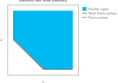
Note that, since a Pareto-optimal solution doesn’t have all objectives better than another optimal solution, they are weakly minimal as well. Therefore, X∗ ⊆ X∗w. Figure 2.4
shows, in a two-objective space, the efficient (lighter and thicker line) and weakly efficient (darker line) fronts of a feasible space. One simple example of the difference is to consider the solutions z1 = [1 0]T and z2 = [1 0.5]T. Clearly the first dominates the second in
the Pareto sense, but since z1 is not smaller than z2 in both components, they are
incomparable according to the weak dominance.
f1 f2
Feasible region Weak Pareto-optima Pareto-optima
Efficiency and Weak Efficiency
Figure 2.4: Weak efficient solutions in a two-objective problem. The weakly minimal
front includes the minimal front and the solutions in the “south” and “west” boundaries.
So, why bother with this dominance anyway? The reason is that some methods for solving multi-objective problems (as will be shown later) have only guarantee to find weak optimal solutions. This is important, because, as mentioned before, they should be avoided if possible. Hence, it is good to see the limitations of these methods before just using them, and this requires the knowledge of the weak efficiency.
2.3.1.2 Proper efficiency
I have mentioned that the weak optimality is generally not useful to take decisions. Well, sometimes, even the Pareto-dominance is too weak for applications. For example, in some cases, it is possible to improve significantly an objective in the expense of an infinitesimal decrease of other. The (limits of) ratios of improvement and deteriorations of these objectives are called trade-off coefficients [6]. Solutions that are efficient and also have a bounded trade-off are called properly efficient. Then, a last concept of optimality that is both useful and complicated is theproper efficiency. One reason for this complication is that there are different definitions for it, and they are not always necessarily equivalent [10]. For that, I will present the definition in the Geoffrion’s sense [8]. See [10] and [7] for some different definitions.
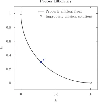
Consider Figure2.5and the Pareto front shown there. From the definition of efficiency, if you are at a minimal point, say,z′in the figure, there is no way of reducing one objective
without increasing another, that is, there is a trade-off. So, assume you start from z′
and begin to move to the left in the Pareto front. When you do that, for each decrease you get for the first objective, the second has to increase a given amount. Because of the slope of the curve, as you approach the solution [0 1]T, equal steps to the left results
will result in an infinite step up. A corresponding effect happens in the other extreme, [1 0]T. In these solutions, one says that the trade-off is unbounded.
z’
0 0.5 1
f1
0 0.2 0.4 0.6 0.8 1
f2
Properly efficient front Improperly efficient solutions
Proper Efficiency
Figure 2.5: Example of properly efficient solutions. Each solution somewhere in
the middle of the front has a finite trade-off when moving to a neighbor. But, when this neighbor approaches the limits, this trade-off becomes infinity. The solutions that provide finite trade-offs are properly efficient, and the extreme ones, improperly efficient.
Now it is possible to define proper efficiency [10].
Definition 7 (Proper efficiency (Geoffrion, 1968)). A feasible solutionx∗p is called prop-erly efficient in the Geoffrion sense if:
• It is efficient; and
• There is a real number M > 0 such that for all i and x ∈ X satisfying fi(x) <
fi(x∗p) there exists an index j such thatfj(x)> fj(x∗p) and
fi(x∗p)−fi(x)
fj(x)−fj(x∗p) ≤
M
If both conditions are satisfied, thenx∗p [and its corresponding image f(x∗p)] is called
properly Pareto optimal, orproperly efficient. If a point satisfies only the first condition, then it is efficient but also called improperly efficient.
The set of all properly minimal solutions is the properly efficient set X∗p in the search
space, and properly efficient front Z∗p in the objective one. Also, according to its
definition, since a properly minimal solution is also efficient, it can be written X∗p ⊆
X∗ ⊆ X∗w.
These types of solutions are more useful for the decision process, both because they are already efficient and because sometimes the limited trade-off property can be use-ful. Also, some methods, under some circumstances, can find weakly optimal points (normally undesirable), but, in different occasions, some properly minimal solutions can be computed (see section 2.4.1). Therefore, it is good to have an idea of this kind of dominance as well.
2.3.2 Boundaries of the Efficient front
Given a feasible objective space, there are some special points that deserve attention.
The first point is called ideal solution, also named shadow minimum in some studies (like [11]), indicated byz⋆. Its components are the individual minima of each objective,
that is,
z⋆ =
min
x∈Xf1(x) minx∈Xf2(x) . . . minx∈Xfm(x) T
If there was a feasible point that minimized at the same time all of the objectives, it would be elected the final solution and there would be no problem in the decision making, that is, it would be anideal situation. However, this is usually not the case in thereal world, so this point is normally attainable only in dreams. See Figure2.6 for a two-dimensional illustration of it.
Opposed to the ideal point, there is the maximal point, defined as
zmax=
max
x∈Xf1(x) maxx∈Xf2(x) . . . maxx∈Xfm(x) T
that is, it is composed of the individual maxima of each function.
Another important solution is theNadir point, defined as
zN adir=
max
x∈X∗f1(x) maxx∈X∗f2(x) . . . xmax∈X∗fm(x)
z⋆
zN adir
zmax
f1
f2
Feasible region Efficient front Ideal point Nadir point Maximal point
Special Points of the Feasible Objective Space
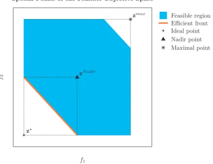
Figure 2.6: This figure shows the ideal, Nadir and maximal points for a given feasible
objective space. Notice that the Nadir is comprised to the efficient set, while the maximal one is computed for all of the feasible space.
The difference between this and the maximal point is that the Nadir solution is limited only to the efficient front (notice that x ∈ X∗ here), as shown in Figure 2.6. While
the first two points are easier to compute because the whole feasible objective set is considered, the computation of the Nadir can get really hard because only the portion of this set that comprises the efficient solutions is taken into account. For two objectives, one can use a pay-off table [8] to calculate it exactly. However, for three or more, this same technique is usually unable to correctly determine its components. Because of this, sometimes just a good approximation for this point can be used. See [9] for more details about this topic. Notice that none of these points needs to be attainable, especially the ideal one.
What is so special about these points? Sometimes, the objectives in a problem represent different things, with distinct measurement units and diverse ranges. Some methods for solving multi-objective problems require the aggregation of all criteria into one, like a weighted sum of the objectives, and it makes no sense to add centimeters with bananas. Moreover, when you have a set of non-dominated points, you may wish to perform some trade-off analysis on them. If one objective ranges from 0 to 1 and the other from 0 to 10,000, any small perturbation in the first (like 0.1) can yield a giant variation in the other (like 100) that is not actually significant for its range.
there are cases when the feasible objective set is unbounded from above, so the maximal point goes to infinite. Also, most of the attention is reserved to the efficient front, so the ideal and Nadir points are most often preferred to standardize the objectives. The
i-th objective can be converted into dimensionless with
˜
fi(·) =
fi(·)−zi⋆
zN adir i −z⋆i
, i= 1,2, . . . , m
wherein the operation fi(·)−zi⋆ means to subtract all thei-th component of the ideal
solution from all possible points of the i-th objective. If these limits are not known
exactly, some good approximations can be adopted instead. “Good” here means “suit-able for your problem”, so it will probably vary a lot from case to case. Only when the objectives are standardized, a discussion about relative importance of criteria, their weights and an interpretation of trade-off coefficients become meaningful.
2.3.3 Shapes of the Efficient front
In this subsection I will consider briefly some characteristics of the efficient front. First, as all of the figures shown so far depict two-objective problems (two dimensions), the Pareto front was always a curve (one dimension). In general, if a problem hasm objec-tives, its minimal front, assuming it exists, will be a (m−1)-dimensional hyper-surface [8]. This is not, however, a rule: there may be some degenerate cases, like a curve in a three-objectives problem, or a single point in a two-criteria one. So, the best that can be said is that the dimension of the efficient front of am-objectives problem will be less
than or equal tom−1.
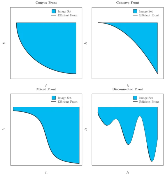
The other consideration is about the shapes the fronts can present. Figure2.7shows the most common encountered in continuous problems. I will describe them in a simple and intuitive way. If you are interested, the reference [8] contains more technical information about this topic.
The top left shows a convex front. It is such that, for any pair of optimal points x∗1
and x∗2, the line going from the first to the second remains entirely in the image of
f1 f2
Image Set Efficient Front
Convex Front
f1 f2
Image Set Efficient Front
Concave Front
f1 f2
Image Set Efficient Front
Mixed Front
f1 f2
Image Set Efficient Front
Disconnected Front
Figure 2.7: Some common shapes of efficient fronts. Top left: convex; top right:
concave; bottom left: mixed (convex and concave); bottom right: disconnected.
The convex front is possibly the most important, since a lot of real-life problems present as efficient front a convex one. Also, many known methods for computing efficient points can only approximate the solutions in the convex portions. This will be shown in the next section.
2.3.4 Solving a Multi-objective Problem
Without further information, they are equally good, so, in principle, all of them should be considered as “the optimal solution”.
However, in practical problems, only one or a few alternatives are effectively imple-mented. Consider the last part of the Perfect Workout example to see that:
Example 2.3 (The perfect workout routine: Part 3). In part 2, Peter formulated Maria’s problem into finding the workout routine that yields the minimum increase in
fat body percentage after 3 months and the smaller effort required. From all eight ex-ercises, 1, 2, 4, 5, 6 and 8 are efficient, and they are shown in Figure 2.8. Even after excluding the non-efficient alternatives, she still needs to choose only one for the next three months. How should she proceed?
1
2
4 5
6
8
0 0.2 0.4 0.6 0.8 1
Effort required
−15 −10 −5
0 5 10
Bo
dy
fat
(%)
Solution for Scenario 1 Solution for Scenario 2 Multi-objective Workout Routine Example
Figure 2.8: Efficient workout routines. Among these alternatives, routine 8 (P90X)
can satisfy Maria’s preferences in Scenario 1, while routine 2 is more preferable in Scenario 2. See the text.
The concept of efficiency says that, assuming no further information is available, the
efficient alternatives are all equally preferable. However, Maria is a human being, so she has different needs and opinions, i.e., she has preferences. She should then pick the solution that pleases her most for a given situation.
Consider the following scenarios:
• Scenario 1: Maria decided to make some money by working as a model in a
bikini’s company, and the pictures start to be shot in 3 months. In that case, she could give more importance to her increase in body fat at the sacrifice of her
• Scenario 2: Maria will visit her grandmother in Canada for three months, during the winter. She (the grandmother) is always complaining how her granddaughter
looks so skinny. Under these circumstances, Maria could give herself a break and prefer a more effortless activity, like exercise 2 (Simple walks, indicated by the
asterisk in Figure 2.8). Maybe doing nothing (number 1) could also be an option, but she might think the increase of body fat is too big compared to the walks, so this last one would be the final solution of this scenario.
Just like Maria can only follow one workout routine per time, an employer usually hires a few people for the job, even tough hundreds of the candidates can be “efficient” according to his criteria; a student cannot sleep and study at the same time; etc. So, finding Pareto-optimal solutions is not enough to finish the decision procedure.
When solving a multi-objective problem, there is a person that [12] is assumed to know the problem in hand and who is able to provide preference information related to the different solutions. This person is calleddecision maker (DM)6. Besides the DM, there is also ananalyst, which may be another person, or a group, or even a computer program responsible for the mathematical modeling and computing sides of the process. His aims are to help the DM in various stages of the optimization. In the workout example, one may elicit Maria as a decision maker, and Peter as the analyst.
Therefore, in this point of view, finding all of the Pareto-optimal solutions is not “solving a multi-objective problem”. Rather, it can be understood as “helping a human decision maker in considering the multiple objectives simultaneously and finding a Pareto-optimal solution that pleases him the most” [12]. It is assumed that the DM prefers efficient solutions, or maybe properly efficient, and the weakly minimal ones should be avoided. But, even so, the Pareto set doesn’t tell which solutions to choose, but which points to avoid. The final solution must have some insight from the DM.
2.4
Methods for Finding Efficient Points
Apart from the discussion of the last section, let us forget about the DM for the rest of this chapter. I will now present here some popular methods for computing optimal solutions for a given multi-objective problem. They are classified asScalarizing Methods, Deterministic Methods without Scalarization and Evolutionary Algorithms. Some of
6
them, like the first, are able to compute sometimes efficient points, but weakly and properly ones can be expected; and others, like the last, provide in the best case a good approximation of the Pareto front, but with no guarantee of optimality. For each one, I will present some characteristics, weaknesses and strengths.
2.4.1 Scalarizing methods
In the scalarizing methods, the functions are combined in order to convert the original multi-objective problem into a single-objective one. In this way, instead of dealing with vectors, one handles scalars. This is a clever approach, because it is possible to use single-objective techniques, which are very well developed.
When the problem is scalarized, the solution of it is a single point. It is then necessary to discuss how this point relates with the solutions of the original problem. More precisely, the following questions can be made [8]:
1. Does the optimization of the scalarized problem always result in an efficient solu-tion of the original one?
2. Converting a vector into a scalar requires the use of some parameters (e.g., aggre-gating its components using a weighted sum demands a vector of weights). Differ-ent parameters may produce distinct solutions. The question is: is it possible to generate all of the minimal solutions by varying these parameters?
3. This question is related to the previous one: assuming the optimization of the scalarized problem yields an efficient point, how does the choice of the parameters control the position of the solution in the Pareto front?
As you may think, each scalarizing method may have a different answer to these ques-tions. I will respond them for each of the techniques presented here.
2.4.1.1 Weighting Method
Also known as linear aggregation, in this method the original vector function is con-verted into a scalar by aggregating its components into a weighted sum, which should be minimized. The original problem then becomes
minimize fw(x) = m X
i=1
wifi(x) (2.6)
subject to Pm
i=1wi= 1
wi ≥0, ∀i= 1,2, . . . , m
x∈ X
whereinwi is the weight for thei-th objective, considered non-negative, and whose sum
over all objectives is assumed7 to be 1. These weights can be viewed as a “relative
importance” of the respective objective. For instance, in the workout example, if Maria thinks that reducing her body fat percentage is more important than decreasing the effort, she can assign w1 = 0.8 for the first and w2 = 0.2 for the second, meaning
roughly “losing body fat deserves 80% of her attention”.
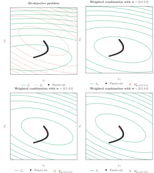
Each vector of weights represents a different problem, so a diverse solution can be ex-pected when you vary them. Figure2.9shows a two-objective example. By changing the relative values of the weights, different problems with distinct solutions are obtained.
Now, let’s get down to business and answer the questions of the introduction. First, are the solutions of the weighted problem always Pareto-optimal? As can be seen in [6, 8], the solutions are weakly Pareto-optimal, but if all of the weights are positive, not just non-negative as is written in (2.6), the solutions are properly Pareto-optimal. If you think a little about that, it does not make much sense to let a weight assume the value zero, because it means that the corresponding objective has no significance at all, so why include it in the first place? Nevertheless, zero weights are still included to make the formulation more general.
Second, can all of the efficient points be found by this method? The answer is a big “yes” followed by “provided the Pareto front is convex”. If the front is convex, for every optimal solutionx∗ there exists a weightwsuch that the weighted problem (2.6) yields x∗ as a solution [6]. Conversely, if the optimal curve is non-convex, there does not exist
any w such that the solution of (2.6) lies in this non-convex portion [13]. Das and
Dennis in [13] show why this sad effect happens.
7
x1 x2
f1 f2 Pareto set Bi-objective problem
x1 x2
fw Pareto set x∗w=[0.8 0.2] Weighted combination with w= [0.8 0.2]
x1 x2
fw Pareto set x∗w=[0.5 0.5] Weighted combination with w= [0.5 0.5]
x1 x2
fw Pareto set x∗w=[0.2 0.8] Weighted combination with w= [0.2 0.8]
Figure 2.9: Solving a two-objective problem by the weighting method. Top left: the
level curves of two quadratic functions and the respective Pareto set. Top right: level curves of the weighted problem with w = [0.8 0.2]T, favoring the first objective; the
‘x’ indicates the solution with this aggregation. Bottom left: same thing, but with w= [0.5 0.5]T, giving the same importance to both objectives. Bottom right: similar,
withw= [0.2 0.8]T, preferring more the second objective.
There are some more considerations to be made in order to answer to the last question. One important thing is that the idea of “relative importance” mentioned before is only validwhen the objectives are dimensionless [9]. So, even for convex problems, when the functions have different ranges, do not expect to have a good control of the position of the solutions by just changing the weights. This is also illustrated in Figure 2.9. The case of equal weights, for instance, does not result in a solution in the middle of the Pareto set because the functions have distinct ranges. This is not stressed enough in many texts, but it is important. As stated before, the standardization usually means computing the ideal z⋆ and the Nadir (or at least a good approximation of it) zN adir
For the other consideration, suppose you want to approximate the whole Pareto front. For that, you must solve the problem (2.6) a lot of times with different options of weights. And there lies the question of how to set their values in order to cover the efficient front. In two dimensions, one can setw1=w,w2 = 1−wand varywup in the interval [0,1].
But for three or more this is not so obvious, because one would need to wander around the whole hyper-surface Pm
i=1wi = 1. There is, however, a related study in [11].
Finally, even if the Pareto front is convex, the functions are normalized and you man-aged to get a uniform distribution of weights for any number of objectives, there is no guarantee that this will yield uniform points in the efficient front [13]. The problem is not just that the final result will not look so nice, but, more important, it is hard to control the location of the solutions (see Figure 2.10). It may be possible that a small perturbation in a weight results in a very far point from the previous one, or even the opposite8.
f1 f2
Efficient front Uniform solutions Uniform weights
Weights distribution×Solutions distribution
Figure 2.10: Generating 10 efficient solutions with uniform weights. The ‘×’
repre-sents solutions obtained by settingw1=wandw2= 1−wand varyingwfrom 0 to 1
in equal increments. For comparison, the circles indicate what is a true equally spaced set of solutions.
In summary, the weighting method is one of the simplest scalarization methods to solve multi-objective problems. Its solutions are weakly Pareto-optimal, and if all of the weights are positive, they are properly optimal. However, only convex portions of the front are reachable, and, even when that is the case, it is hard to control the location of the solutions.
8
A lot of details were provided here about this method. The goal is not defame it, but more to warn analysts of its limitations before, for example, blindly summing all objectives and hoping to get a solution in the middle of the front.
2.4.1.2 ǫ-constraint Method
In theǫ-constraint method, also calledCompromise Programming [8], one function, say,
fk, is chosen to be minimized, while the otherm−1 receive upper bounds ǫi, wherein
i= 1,2, . . . , mandi6=k. So,m−1 new constraints are introduced in the problem, and
the original multi-objective one becomes
minimize fk(x) (2.7)
subject to fi(x)≤ǫi, i= 1,2, . . . , m, i6=k
x∈ X
To get an idea of how this works, check the Figure2.11. If f2 receives the upper limit
ǫ1, the minimization off1 generates the pointx∗ǫ1, whose image is shown as a square in
the figure. Iff2 gets a different bound ǫ2, another solutionx∗ǫ2 is obtained. By varying
the bounds of the m−1 remaining objectives, different points are obtained.
In principle, any function can be chosen to be minimized, and the solutions of (2.7) areweakly efficient with regard to the original problem [6]. In order to answer the first question, there are, nevertheless, ways of guaranteeing efficiency instead of just weak efficiency [6]. If a pointx∗ is the solution of the ǫ-constraint problem solved varying k
from 1 to m, that is, each time minimizing one different objective and with the same
vector [ǫ1 ǫ2 . . . ǫm]T of upper limits, than it is Pareto optimal. Alternatively, if it can
be shown thatx∗ is a unique solution of (2.7) with a given value ofk, then it is Pareto
optimal.
The verification that a point is a unique solution of a problem is hard (unless the front is convex), and solving m different problems in order to get just one efficient solution
may be a big price to pay, principally when there is a great number of objectives. The advantage of this method is that, theoretically, any minimal solution can be found, even the ones in non-convex portions. This answers the second question made before.
If someone desires to approximate the whole front using this method, it can be accom-plished by setting different upper bounds ǫi. Of course, there is a chance of adjusting
f2=ǫ1
f2=ǫ2
f(x∗
ǫ1)
f(x∗
ǫ2)
f1 f2
Pareto front
ǫ-Constraint Method
Figure 2.11: Two-objective example solved by theǫ-Constraint method. Here, f1 is
minimized andf2receives upper limits. Whenf2needs to be smaller or inferior thanǫ1,
minimizingf1 generates the solutionx∗ǫ1. A similar reasoning applies to whenf2≤ǫ2.
(so the solutions are always the same). In order to not waste time with these degenerate cases [8], the ideal and the Nadir points are required again. So, these two points create a hyper-box limiting the Pareto front, and a hyper-grid can be created by varying the vector of constraints inside it. This technique provides a better control of points than the weights do, but, depending on the front’s shape, even a uniform grid cannot guarantee uniform solutions.
The ǫ-constraint method beats the weighting method with its ability of approximating
2.4.1.3 Weighted Metrics
In the Weighted Metrics method9 a different approach is pursued. In the weighting
method, one deals with preferences in the objectives, and in the ǫ-constraint, upper bounds are adopted. Here, the concept ofaspiration levels is introduced.
These levels are simply the desires one may have for each objective. For example, a student may wish to score 95% of his efficiency index and sleep during 8 hours per night. Also, Maria can decide to lose 20% of body fat and do only 0.2 of effort. More generally, one may opt for the levelzr1 in objectivef1,z2rin objective f2, and so on, and
then he has a reference point zr = [zr1 z2r . . . zrm]T. The idea is then to get a solution
that is the closest possible to this point. This is a more natural way of thinking, and should be a good reason to popularize this method. However, it hasn’t received the importance it apparently deserves. I will point some reasons for it in the end of this section.
There are some definitions of “getting close” to a reference point [9]. In this method, this is translated as “finding the point with the smallest distance to zr” or, more generally,
with the smallest value of a metric. The Lk metrics, or Minkowski distance, or even
norms, adopted here, are defined as
Lk(f(x),zr) =kf(x)−zrkk, k= 1,2, . . . ,∞ (2.8)
in which, if 1≤k <∞, equation (2.8) takes the form
kf(x)−zrkk= "m
X
i=1
(f(x)−zr)k
#1/k
, 1≤k <∞
and, ifk=∞, the distance is called Tchebycheff norm, and assumes the form
kf(x)−zrk∞= max
i∈{1,2,...,m}|fi(x)−z r i|
Therefore, the original multi-objective problem is converted in a scalar one by minimizing a weighted metric in the following way:
9
It is also called “compromise programming” in [6] and “distance to a reference point” in [8]. The first one is the same as the one attributed to theǫ-constraint method (this reflects how the literature
minimize Lk(f(x),zr,w) =kwT(f(x)−zr)kk (2.9)
subject to Pm
i=1wi= 1
wi≥0
x∈ X
for a given reference point zr, a vector of weights w = [w1 w2 . . . wm]T and a given
metric valuek. These weights are, in principle, used to normalize functions with different
ranges, but, if this was already done10, they can be used to generate different solutions.
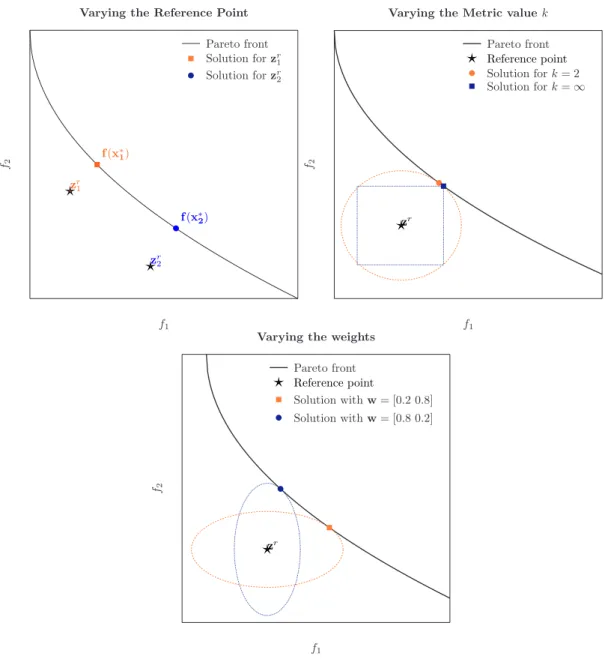
The ways one can create different solutions are by: (i) changing the reference point; (ii) setting a new metric valuek; and (iii) varying the weights. Some examples are shown in Figure2.12. For a given reference point, this method tries to get close to it according to different metrics and sets of weights. This technique is very simple, and the figures show how it can be versatile. However, the answers to those three questions will probably dry out the fantasy.
First of all, the solution to the weighted metric (2.9) is not always Pareto optimal. Sometimes even dominated solutions are obtained. For example, if you choose a reference point that is feasible and not optimal, then the distances in (2.9) will have their minimum value (equal to zero) in exactly the (not efficient) reference point. There is a lemma [8] that says that, in order to avoid dominated solutions, the reference point should be the ideal point z⋆ or any other such that zr ≺z⋆. Please note that this is not a necessary
condition, since sometimes minimal points can be obtained even if zr is dominated by
the ideal point, as the examples of Figure 2.12 show. Nevertheless, most books already usez⋆ in place to zr in the formulation (2.9).
So, from now on, assume the reference point satisfies the condition above. Now, are the solutions of (2.9) efficient in the original problem? The answer is [6]:
• If the metric used is finite (that is, 1≤k <∞), then, if a solution x∗ is unique (a
hard thing to test) or the weights are all positive, then it is efficient;
• If the Tchebycheff metric is in use, then if a solution x∗ is unique, it is efficient.
And if the weights are all positive, then the solution isweakly efficient.
It seems here that the Tchebycheff has a disadvantage with regard to the other metrics. But, what about the possibility of generating any solution in the front? This is where
10
zr
1
f(x∗1)
zr 2
f(x∗2)
f1
f2
Pareto front Solution forzr
1
Solution forzr
2
Varying the Reference Point
zr
f1
f2
Pareto front
Reference point
Solution fork= 2 Solution fork=∞
Varying the Metric valuek
zr
f1
f2
Pareto front
Reference point
Solution withw= [0.2 0.8] Solution withw= [0.8 0.2] Varying the weights
Figure 2.12: Generating different solutions in the Weighted Metrics method. Top
left: changing the reference point and keeping the rest constant. Top right: using a different metric. Bottom: varying the weights.
this infinite norm excels: if 1 ≤k <∞, then solutions in the non-convex region of the front are not obtained, even if an ideal reference point is used. And if k = ∞, any solution can be generated in any part of the front - but be prepared to get some weak optimal ones.
Finally, if zr =z⋆ or better and the Tchebycheff metric is used (or any other and the