Multi-objective optimization with Kriging surrogates using “moko”, an open source package

Multi-objective optimization with Kriging surrogates using “moko”, an

open source package

Abstract

Many modern real-world designs rely on the optimization of multiple competing goals. For example, most components designed for the aerospace industry must meet some conflicting expectations. In such applications, low weight, low cost, high reliability, and easy manufacturability are desirable. In some cases, bounds for these requirements are not clear, and performing mono-objective optimizations might not provide a good landscape of the required optimal design choices. For these cases, finding a set of Pareto optimal designs might give the designer a comprehensive set of options from which to choose the best design. This article shows the main features and functionalities of an open source package, developed by the present authors, to solve constrained multi-objective problems. The package, named moko (acronym for Multi-Objective Kriging Optimization), was built under the open source programming language R. Popular Kriging based multi-objective optimization strategies, as the expected volume improvement and the weighted expected improvement, are available in the package. In addition, an approach proposed by the authors, based on the exploration using a predicted Pareto front is implemented. The latter approach showed to be more efficient than the two other techniques in some case studies performed by the authors with moko.

Keywords

Multi-Objective Optimization, Surrogate Model, Kriging, Open Source Package

1 INTRODUCTION

Multi-objective optimization is a field of interest in many real-world applications. Engineering design has multiple and conflicting goals and, most of the time, the relationship between the decision space (design variables domain) and the outcome is highly complex. Around the 2000’s, some comprehensive reviews were made that cover many of the basic ideas and challenges related to many-objective optimization (Van Veldhuizen and Lamont, 1998; Zitzler, 1999; Deb et al., 2002b). Today, there are many efficient algorithms for dealing with multi-objective optimization, most of them based on evolutionary techniques (evolutionary multi-objective optimization algorithms – EMOAs). Some state-of-the-art algorithms can be found in Corne et al., (2001); Zitzler et al., (2001); Deb et al., (2002a); Emmerich et al., (2005); Beume et al., (2007); Deb, (2014); Chen et al., (2015). However, even when using such efficient frameworks, if the evaluation of the designs is too time consuming, a surrogate approach is usually used to alleviate the computational burden.

To address this issue, the present authors have developed an open-source package based on Kriging interpolation models. The package, named moko (acronym for Multi-Objective Kriging Optimization), is written in R language and presents three multi-objective optimization algorithms: (i) MEGO, in which the efficient global optimization algorithm (EGO) is applied to a single-objective function consisting of a weighted combination of the objectives, (ii) HEGO, which involves sequential maximization of the expected hypervolume improvement, and (iii) MVPF, an approach based on sequential minimization of the variance of the predicted Pareto front. The first two are implementations of well-known approaches of the literature, and MVPF is a novel technique first presented in Passos and Luersen (2016) and in Passos and Luersen (2018), in which a composite panel with curved fibers is optimized for multiple objectives.

In R language, packages are the fundamental units of reproducible codes. They must include reusable R functions, the documentation that describes how to use them and sample data. For developing the moko code, the

Adriano Gonçalves dos Passosa* Marco Antônio Luersena

a _{Laboratório de Mecânica Estrutural (LaMEs),}

Universidade Tecnológica Federal do Paraná (UTFPR), Curitiba, PR, Brasil. E-mail:

adriano.utfpr@gmail.com, luersen@utfpr.edu.br

*Corresponding author

http://dx.doi.org/10.1590/1679-78254324

authors followed the guidelines and good practices provided by Wickham (2015). This resulted in a package that has been accepted and is available at the Comprehensive R Archive Network (CRAN), the official public repository for R packages.

We highlight that the present paper is a revised and extended version of the work presented in the conference MecSol2017 (Passos and Luersen, 2017b).

2 SURROGATE MULTI-OBJECTIVE APPROACHES 2.1 Kriging Basics

Kriging is a spatial interpolation method and was originated in the field of geosciences (Krieg, 1951). Given a black box function

y D

:





d





, we can model it as being a realization of a stochastic process



 

x x

,



D

. The idea of Kriging is to predict unknown values of

y

 

x

based on the conditional distribution of



 

x

given some priori knowledge. This priori knowledge comes from a finite set of n-observations of

y

 

x

. In practical terms, the Kriging surrogate model can be seen simply as the following Gaussian random field

 

_{x |}

_

 

_{X y}

_

_



_

_m

 

_{x ,}

_

2 _s2

 

_x



   (1)

where

x





x

1

, ,



x

d



 

D



d is any design inside the project domain;

X





x

 1

, ,



x

 n



is a matrix

containing initial known design points (usually called design of experiments (DOE));

y





y

 

x

 1

, ,



y

 

x

 n



T are the true responses evaluated at X and

m

 

x

and

s

2

 

x

are scalar fields representing the mean and variance which define the Gaussian random field.

The process of building the mean and variance descriptors for the Gaussian field is well covered in the literature (Sacks et al., 1989; Jones et al., 1998; Forrester et al., 2008; Roustant et al., 2012; Scheuerer et al., 2013).

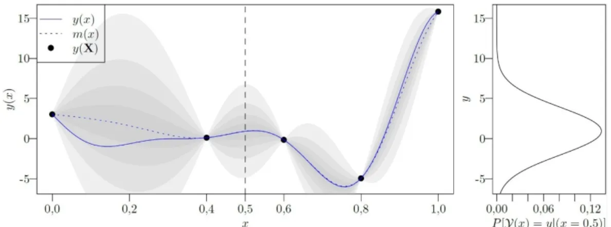
To illustrate the Kriging surrogate, consider the unidimensional scalar function given by

  



2





6 2 sin 12 4

y x  x x (2)

which is evaluated at the following DOE points: X



         

0.0 , 0.4 , 0.6 , 0.8 , 1.0



. The Kriging model for this case is presented in Figure 1. In this figure, the unknown exact function is depicted in bold line and

m x

 

(the predictor’s mean value) in dashed line. A section view is drawn on the right side to show the probability density of

 

x |



 

X  y



  for

x

0.5



.

Figure 1: Example of a Kriging surrogate for a scalar mono-variable function.

these subjects in Forrester et al. (2008). The Kriging models are built using the DiceKriging R package (Roustant et al., 2012).

2.2 The MOKO paradigm

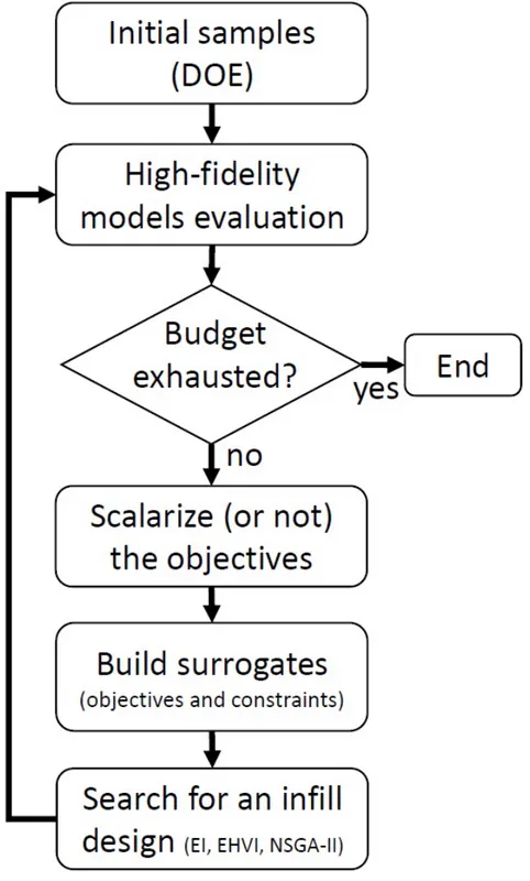
Most of surrogate-based multi-objective algorithms uses an iterative approach. The most common framework is to interactively search for infill points that maximizes some search criteria (like the expected improvement EI). All algorithms implemented in ‘moko’ follows that paradigm and Figure 2 shows the workflow of ‘moko'.

2.3 Multi-Objective Efficient Global Optimization (MEGO)

The efficient global optimization algorithm (EGO) was proposed by Jones et al. (1998) for mono-objective optimization. It consists in, from an initial set of samples

X

, a Kriging model is built using the responses of a high-fidelity model1_{, and EGO sequentially maximizes the expected improvement (EI) and updates the model at each}

iteration (including re-estimation of the hyperparameters).

The basic idea of the EI criterion is that by sampling a new point

x

 _{the results will be improved by}

 

min

y y x _if

 

min

y x  y _or

0

_{otherwise, where}

min

y

is the lowest value of the responses

y

obtained so far. Obviously, the value of this improvement is not known in advance because y

 

x _{is unknown. However, the}

expectation of this improvement can be obtained using the information from the Kriging predictor. The EI criterion has important properties for sequential exploitation and exploration (filling) of the design space: it is null at points already visited (thus preventing searches in well-known regions and increasing the possibility of convergence) and positive at all other points, and its magnitude increases with predicted variance (favoring searches in unexplored regions) and decreases with the predicted mean (favoring searches in regions with low predicted values).

The EGO algorithm can be easily adapted to a multi-objective framework by scalarizing the objective vector into a single function (Knowles, 2006). The constrains of the optimization problem can be considered simply by building independent metamodels for each constraint and multiplying the EI of the composed objective function by the probability of each constraint to be met (Sasena et al., 2002). The MEGO algorithm can be summarized as follows:

1. Generate an initial DOE

X

using an optimized Latin hypercube;

2. Evaluate

X

using high-fidelity models and store responses of f , , , 



_{f f1 2}  _fm





and

g

, , ,





_

g g

_{1 2}



g

_p



_

 for the

m

-objectives and

p

-constraints;

3. while computational budget not exhausted do:

(a) Normalize the responses to fit in a hypercube of size

 

0,1 m ;

(b) For each

x X



compute a scalar quantity by making

f

_



max





_{i i}

f



 

 

_{i i}

f

, where



is drawn uniformly at random from a set of evenly distributed unit vectors and



is an arbitrary small value which we set to

0.05

; (c) Build Kriging models for

f

and for the constraints

g

;

(d) Find

x

 that maximizes the constrained expected improvement: x arg max EI



_C

 

x



_;

(e) Evaluate the “true” values of f x

 

 _{and g}

 

_x _{using high-fidelity models and update the database.}

4. end while

More details regarding scalarization functions like sampling



can be found in Miettinen and Mäkelä (2002), Nikulin et al. (2012) and Ruiz et al. (2015). The parameter





0

, which must be a small positive value, is the so-called augmentation coefficient and it is used to assure the Pareto optimal solution can be found for any reference point (Ruiz et al. 2015).

Here, in order to handle the constrains, the EI is computed using a custom modified version of the DiceOptim::EI function provided in Ginsbourger et al. (2013). In addition, in all approaches, the optimized Latin hypercube is built using the R package lhs (Carnell, 2012).

2.4 Expected Hypervolume Improvement (EHVI – HEGO)

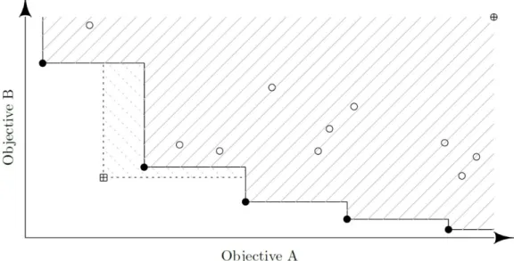
The hypervolume improvement (EHVI) infill criterion is based on the theory of the hypervolume indicator (Zitzler and Thiele, 1998), a metric of dominance of non-dominated the solutions have. This metric consists in the size of the hypervolume fronted by the non-dominated set bounded by reference maximum points. Figure 3 illustrates this concept for two objectives. The hollow circles points represent dominated designs, while the filled ones represent Pareto optimal solutions. The area hatched with solid lines is the dominated portion of the objective space, while the area hatched with dashed lines represents the area that would be additionally dominated when a new observation (the crossed square point) is added. This additional ‘area’ is called the hypervolume improvement (since it can be generalized for more than two objectives).

1 _{High-fidelity model is a detailed model, usually computationally expensive, to represent the problem we are studying. From the simulation}

Figure 3: Hypervolume improvement concept.

The EHVI is thus the expected improvement at the hypervolume size we would get by sampling a new point

x

_{. Here, the EHVI is computed using the R package GPareto (Binois and Picheny, 2016). The original GPareto::EHI}

function does not account for constrains, so a custom modification was implemented (available in the moko package). The algorithm used here (HEGO – Hyper Efficient Global Optimization) is similar to the MEGO algorithm and can be summarized as follows:

1. Generate an initial DOE

X

using an optimized Latin hypercube;

2. Evaluate

X

using high-fidelity models and store responses of f , , , 



f f_{1 2}  f_m



 and

g

, , ,





_

g g

_{1 2}



g

_p



_

 for the

m

-objectives and

p

-constraints;

3. while computational budget not exhausted do:

(a) Normalize the responses to fit in a hypercube of size

 

0,1 m ;

(b) For each of the

m

-objectives and

p

-constraints, build a Kriging model;

(c) Find

x

 that maximizes the constrained expected hypervolume improvement: x arg max EHVI



_C

 

x



_;

(d) Evaluate the “true” values of f x

 

 _{and g}

 

_x _{using high-fidelity models and update the database.}

4. end while

For this and the previous approach, a simulated annealing (SA) algorithm is used to maximize the infill criteria. SA algorithm is provided by the R package GenSA (Xiang et al., 2013).

2.5 Minimization of the Variance of the Kriging-Predicted Front (MVPF)

The MVPF technique is based on iterative improvement of the fidelity of the predicted Pareto set. The idea is to build a Pareto front from a given initial set of Kriging models (one for each cost or constraint function) using the mean of the predictor of each model as the input function. From the estimated front

P

, the design with higher variance

x

 _{(i.e., the most isolated in the decision space) has its “true” value evaluated using the high fidelity model.}

A new set of Kriging models is then rebuilt, and the process is repeated until a stopping criterion is met. The MVPF algorithm can be summarized as follows:

1. Generate an initial DOE

X

using an optimized Latin hypercube;

2. Evaluate

X

using high-fidelity models and store responses of f , , , 



f f_{1 2}  f_m



 and

g

, , ,





_

g g

_{1 2}



g

_p



_

 for the

m

-objectives and

p

-constraints;

3. while computational budget not exhausted do:

(a) For each of the

m

-objectives and

p

-constraints, build a Kriging model;

(c) Find

x





P

that maximizes the variance of the Kriging predictor: x arg max s



_km

 

x



_;

(d) Evaluate the “true” values of f x

 

 _{and g x}

 

 _{using high-fidelity models and update the database.}

4. end while

NSGA-II, proposed by Deb et al. (2002a), is an improved version of the NSGA (Non-dominated Sorting Genetic Algorithm), proposed by Srinivas and Deb (1994). The NSGA-II implementation used here is the one provided in the R package ‘mco’ (Mersmann, 2014). We highlight that instead of NSGA-II another efficient multi-objective algorithm could be employed.

3 MOKO PACKAGE: SOME FEATURES AND USAGE

The installation of ‘moko’ package can be done simply by downloading it from CRAN servers and running the following commands:

install.packages('moko') library(moko)

To make use of any of the three multi-objective optimization algorithms implemented in moko package, the first step is to create a set of initial sampling points (the DOE - design of experiments). This can be done in different ways, however, we suggest employing an optimized Latin hypercube. A randomly generated unit Latin hypercube of dimension k with n samples can be created using only base functions of R by running:

doe <- replicate(k, sample(0:n, n))/n

Alternatively, an optimized Latin hypercube can be generated using the R package lhs (Carnell, 2012) by running:

doe <- lhs::optimumLHS(n, k)

The second step (also common for all algorithms) is to evaluate the high fidelity model responses (objectives and constrains) at the DOE points. The way moko was built, for all algorithms it is expected a single function that returns a vector of responses. If the user has multiple functions for the objectives and constraints, they must be combined into a single one as:

fun <- function(x){ f1 <- objective1(x) f2 <- objective2(x) f3 <- objective3(x) g1 <- constraint1(x) g2 <- constraint2(x) return(c(f1, f2, f3, g1, g2)) }

Note that fun expects, as input argument, a single design vector

x

. Then, the cost functions are evaluated at each point of the DOE by running:

res <- t(apply(doe, 1, fun))

Thereafter, with the output and the DOE, the Kriging models can be built. For this, the authors developed an object class named mkm (multi-objective Kriging model). This object is a structured list of km objects (Kriging models from the DiceKriging package). For instance, to build a mkm object for a fun that returns the first three values as objectives can be created by:

model <- mkm(doe, res, modelcontrol = list(objective = 1:3))

Note that if the objective slot of the modelcontrol list is NULL (i.e., the index of the objectives are not provided) the function assigns that every response of fun is an object (i.e. unconstrained multi-objective optimization problem). On the other hand, if the user inputs the indexes for the objectives, the algorithm assumes the remainder responses are constrains.

Now, to run nsteps iterations of the implemented methods for an object of class mkm, the following should be executed:

new_model_MEGO <- MEGO(model, fun, nsteps) new_model_HEGO <- HEGO(model, fun, nsteps) new_model_MVPF <- MVPF(model, fun, nsteps)

Further details can be found in the help page of each function. For example, the help page of MVPF function can be loaded through the following command:

4 EXAMPLES

Two analytical examples selected from the literature are used to access the robustness of the proposed multi-objective optimization frameworks. These examples are easy-to-compute optimization problems, which allows comparisons with a direct optimization approach performed here by the NSGA-II algorithm.

The quality of the Pareto sets found is compared using the inverted generational distance (IGD) metric (Shimoyama et al., 2013). The IGD can be defined as





1



 



IGD ,

min

,

,

t

d

_







T

T P

T

t p

p P (3)

where

T

and

P

are the true and the current Pareto sets,

T

is the number of designs in the true Pareto set and

t

and

p

are normalized vectors of length m of the m-objectives of the true and the actual Pareto sets, respectively, and

d

 



is a distance metric (in this case the Manhattan distance metric). Hence, the IGD corresponds to the average distance between all designs in the true set and the closest design of the current set. Thus, the lower the IGD, the better the method is.

4.1 Binh and Korn Problem

The Binh and Korn optimization problem is defined as (Binh and Korn, 1997): find:

{ , | 0 5 0 3}

x x

1 2

    

x

1

x

2

to minimize:

f

1



4

x

12



4

x

22

and: f2 



x15

 

2 x25



2

subject to:





2 2

1 1 5 2 25

g  x  x 

and: g2 



x18

 

2 x23



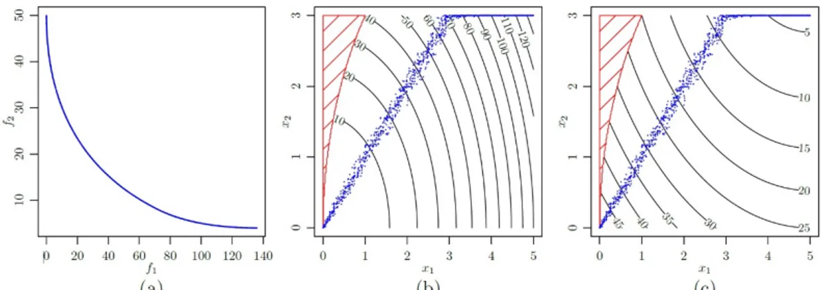
2 7.7

For this example, the “true” Pareto front is obtained by direct optimization using the NSGA-II algorithm with a population size of

500

over

100

generations. The resulting near-uniform Pareto set for

T



500

is shown in Figure 4.

Figure 4. Approximated true Pareto front (obtained with NSGA II) for the Binh and Korn example.

Implementation

Since the Binh and Korn function (and several others) is already implemented in moko package, to generate the “true” Pareto front we use the NSGA-II algorithm simply running the following:

fun.fn <- function(x) fun(x)[1:2] fun.cons <- function(x) - fun(x)[-(1:2)]

tpf <- mco::nsga2(fun.fn, lower.bounds = c(0,0), upper.bounds = c(1,1), constraints = fun.cons,

idim = 2, odim = 2, cdim = 2, popsize = 500)

Note that the domain was scaled to the unit square, thus the input must be multiplied by

 

5, 3

. This step is optional, however, it is highly recommended since it makes the code cleaner.

To pass the constraints to the NSGA-II optimizer one must first split the function by creating an objective function and a constraint function. Both functions receive a vector x with size 2 and also return vectors with size 2. Also, mco::nsga2 consider a violation of the constraint if the return argument is lesser than

0

. This is the reason for the minus sign preceding fun(x) in fun.cons.

For this example, we chose a computational budget of 60 high-fidelity model evaluations. Of these 60 evaluations, 15 are spent building the initial DOE using an optimized Latin hypercube and the remainder are used to generate infill points. In each run, the same DOE is used for the three strategies to avoid random effects caused by different DOEs. This routine is implemented as follows:

n0 = 15 n1 = 45 d = 2

doe <- lhs::optimumLHS(n = n0, k = d) res <- t(apply(doe, 1, fun))

model <- mkm(doe, res, modelcontrol = list(objectives = 1:2)) model_MEGO <- MEGO(model, fun, n1, quiet = FALSE)

model_HEGO <- HEGO(model, fun, n1, quiet = FALSE) model_MVPF <- MVPF(model, fun, n1, quiet = FALSE)

Results

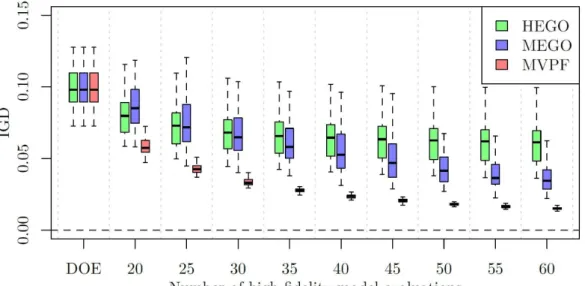
For each strategy, 50 independent runs are performed. Figure 5 shows the IGD histories during the optimization problem. For each run, the IGD values are averaged every five evaluations to avoid overcrowding the graph. The resulting data, gathered from the 50 independent runs, are represented by boxes. The median is shown as a bold horizontal line, and the whiskers correspond to ±1.5 IQR (interquartile range).

Figure 5. History of 50 independent runs of each proposed algorithm for the Binh and Korn optimization problem.

Of the three Kriging-based strategies, MVPF presented, in all iterations, the lowest values for the IGD criterion. The final IGD results for the three techniques are: MVPF



0.0150 0.001



, MEGO



0.0370 0.012



and HEGO

0.0610 0.016

The average number of designs for estimating the Pareto fronts were 49.38 for HEGO, 35.36 for MEGO and 46.9 for VMPF.

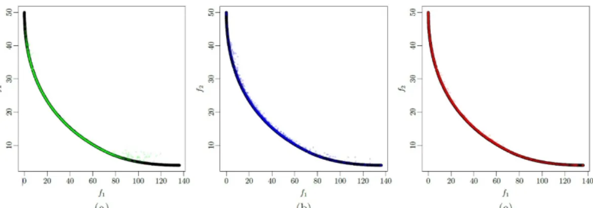
Figure 6: True Pareto front (in black) for the Binh and Korn optimization problem and Pareto fronts obtained using ‘moko’ algorithms (a) HEGO (green), (b) MEGO (blue) and (c) MVPF (red).

4.2 The Nowacki Beam

Based on a problem described by Nowacki (1980), the aim is to design a tip loaded cantilever beam (see Figure 7) for minimum cross-sectional area

A

and minimum bending stress



. The beam length is

l

1 500 mm



and it is subject to a tip load force of

F



5000 N

. The cross-section of the beam is rectangular, with breadth

b

and height

h

, which are the design variables. The design is constrained by five requisites and the optimization problem can be formally defined as the following:

find:



b h

, |1 0

  

b

5 50

 

h

250 ,



to minimize A:

A bh



,

and B:

6 ,

Fl

₂

b h





subject to 1:

3

3

4

Fl

_5,

Ebh







2:

6

₂

Fl

240,

b h







3:

3

120,

2

F

bh







4:

AR

h

10,

b

 

and 5: crit 2 2

4

1

_{2 ,}

1

T Z

F

GI EI

F

l









where



3 3



_/12

T

I  b h hb and

 

3 _/12 Z

Figure 7: The Nowacki beam problem.

The material of the beam is a mild steel with yield stress



Y

240 MPa



, Young’s modulus

E

216.62 GPa



, Poisson ratio



0.27



and shear modulus G = 86.65 GPa. For consistency, all values are physically interpreted in the unit system



mm, N, MPa



. For this problem, the “true” Pareto front is obtained by direct optimization using the NSGA-II algorithm with a population size of 500 over 100 generations. The resulting near-uniform Pareto set for

T

500



is shown in Figure 8.

Figure 8: Approximated true Pareto front for the Nowacki beam problem (obtained with NSGA II).

Implementation

The Nowacki beam problem is also available in moko package. By default, the domain of nowacki_beam function is defined in the unit square. The box parameter can be used to define the actual domain where the unit square will be mapped. This can be done with the following code:

library(moko)

fun <- function(x) nowacki_beam(x, box = data.frame(b=c(10,50), h=c(50,250))) fun.fn <- function(x) fun(x)[1:2]

fun.cons <- function(x) - fun(x)[-(1:2)]

tpf <- mco::nsga2(fun.fn, lower.bounds = c(0,0), upper.bounds = c(1,1), constraints = fun.cons,

idim = 2, odim = 2, cdim = 5, popsize = 500)

For this example, a computational budget of 80 high-fidelity model evaluations is set. Of these 80 evaluations, 20 are spent building the initial DOE using an optimized Latin hypercube and the remainder are used with infill points. In each run, the same DOE is used for the three strategies to avoid random effects caused by different DOEs. This routine is implemented as follows:

n0 = 10 n1 = 60 d = 2

res <- t(apply(doe, 1, fun))

model <- mkm(doe, res, modelcontrol = list(objectives = 1:2)) model_MEGO <- MEGO(model, fun, n1, quiet = FALSE)

model_HEGO <- HEGO(model, fun, n1, quiet = FALSE) model_MVPF <- MVPF(model, fun, n1, quiet = FALSE)

Results

For this example, the results are arranged similar to the previous one and are shown in Figure 9.

Figure 9: History of 50 independent runs of each proposed algorithm for the Nowacki beam optimization problem.

Of the three Kriging-based strategies, MVPF presented, in all iterations, the lowest values for the IGD criterion. The final IGD results for the three techniques are: MVPF = 0.0150±0.001, MEGO = 0.0380±0.005 and HEGO = 0.0420±0.010. The Pareto fronts obtained can be seen in Figure 10. The three algorithms performed similarly to what is observed in Figure 5.

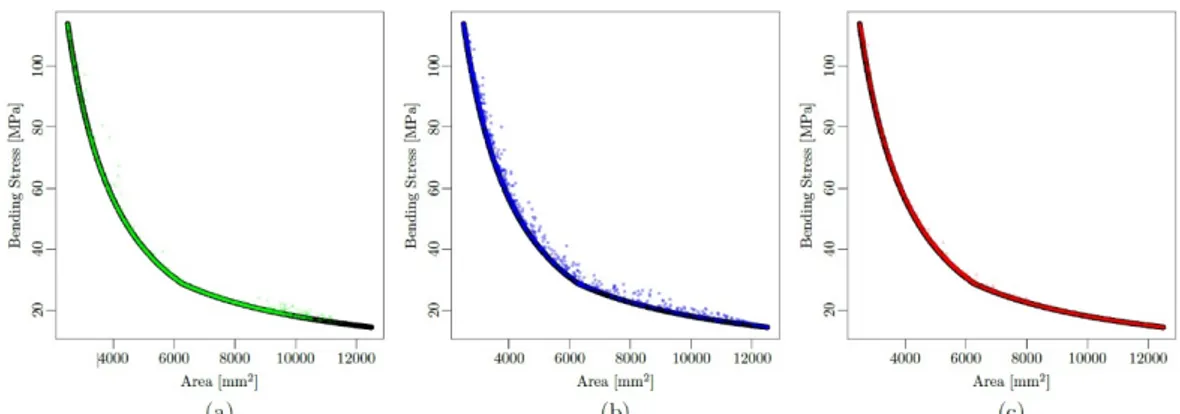
Figure 10: True Pareto front (in black) for the Nowacki beam optimization problem and Pareto fronts obtained using ‘moko’ (a) HEGO, (b) MEGO and (c) MVPF.

Also, the average number of designs on the estimated Pareto fronts were 43.8 for HEGO, 23.56 for MEGO and 48.48 for VMPF.

4.3 Car-side Impact Problem

The mathematical formulation of the problem is presented in Jain and Deb (2014) and is reproduced here as follows:

bounded by:

0.500

 

x

1

1.500,

2

0.450



x



1.350,

3

0.500



x



1.500,

4

0.500



x



1.500,

5

0.875



x



2.625,

6

0.400



x



1.200,

7

0.400



x



1.200,

to minimize

f

1

 

x

:

1.98 4.9



x

1



6.67

x

2



4.01

x

4



1.78

x

5



0.00001

x

6



2.73

x

7

and

f

2

 

x

:

F

and

f

3

 

x

:

0.5



V

MBP



V

FD



subject to

g

1

 

x

:

1.16 0.3717



x x

2 4



0.0092928

x

3



1

,

 

2

:

g

x

0.261 0.0159



x x

1 2



0.06486

x

1



0.019

x x

2 7



0.0144

x x

3 5



0.0154464

x

6



0.32,

 

3

:

g

x

5 1 1 2 6 2 7 3 3 5 6 2

0.214 0.00817



x



0.045195

x



0.0135168

x



0.03099

x x



0.018

x x



0.007176

x



0.023232

x



0.00364

x x



0.018

x



0.32,

 

4

:

g

x

2

2 3 7 2

0.74 0.61



x



0.031296

x



0.031872

x



0.227

x



0.32,

 

5

:

g

x

28.98 3.818



x

3



4.2

x x

1 2



1.27296

x

6



2.68065

x

7



32,

 

6

:

g

x

33.86 2.95



x

3



5.057

x x

1 2



3.795

x

2



3.4431

x

7



1.45728 32,



 

7

:

g

x

46.36 9.9



x

2



4.4505

x

1



32

 

8

:

g

x

F



4.72 0.5



x

4



0.19

x x

2 3



4,

 

9

:

g

x

V

MBP



10.58 0.674



x x

1 2



0.67275

x

2



9.9,

 

10

:

g

x

V

FD



16.45 0.489



x x

3 7



0.843

x x

5 6



15.7

.

This problem aims at minimizing the weight of car and at the same time minimize the pubic force experienced by a passenger and the average velocity of the V-Pillar responsible for withstanding the impact load. All the three objectives are conflicting, therefore, a three-dimensional trade-off front is expected. There are ten constraints involving limiting values of abdomen load, pubic force, velocity of V-Pillar, rib deflection, etc. There are seven design variables describing thickness of B-Pillars, floor, crossmembers, door beam, roof rail, etc.

Implementation

The so called ‘car-side impact problem’ (Jain and Deb, 2014) is not yet implemented on ‘moko’ (but it will be available in a future update). However, building this analytical function in R is simple:

car <- function(x){ if(!is.matrix(x)) x <- t(as.matrix(x)) if(ncol(x) != 7)

stop('x must be a vector of length 7 or a matrix with 7 columns') x1 <- x[,1]

x2 <- x[,2] x3 <- x[,3] x4 <- x[,4] x5 <- x[,5] x6 <- x[,6] x7 <- x[,7]

f <- 4.72 - 0.19*x2*x3 - 0.5*x4

vfd <- 16.45 - 0.489*x3*x7 - 0.843*x5*x6

f1 <- 1.98 + 4.9*x1 + 6.67*x2 + 6.98*x3 + 4.01*x4 + 1.78*x5 + 0.00001*x6 + 2.73*x7 f2 <- f

f3 <- 0.5*(vmbd + vfd)

g1 <- 1.16 - 0.3717*x2*x4 - 0.0092928*x3 - 1

g2 <- 0.261 - 0.0159*x1*x2 - 0.06486*x1 - 0.019*x2*x7 + 0.0144*x3*x5 + 0.0154464*x6 - 0.32

g3 <- 0.214 + 0.00817*x5 - 0.045195*x1 - 0.0135168*x1 + 0.03099*x2*x6 - 0.018*x2*x7 + 0.007176*x3 + 0.023232*x3 - 0.00364*x5*x6 - 0.018*x2^2 - 0.32

g4 <- 0.74 - 0.61*x2 - 0.031296*x3 - 0.031872*x7 + 0.227*x2^2 - 0.32 g5 <- 28.98 + 3.818*x3 - 4.2*x1*x2 + 1.27296*x6 - 2.68065*x7 - 32 g6 <- 33.86 + 2.95*x3 - 5.057*x1*x2 - 3.795*x2 - 3.4431*x7 + 1.45728 - 32 g7 <- 46.36 - 9.9*x2 - 4.4505*x1 - 32

g8 <- f - 4 g9 <- vmbd - 9.9 g10 <- vfd - 15.7 if(nrow(x) == 1)

return(c(f1, f2, f3, g1, g2, g3, g4, g5, g6, g7, g8, g9, g10)) else

return(rbind(f1, f2, f3, g1, g2, g3, g4, g5, g6, g7, g8, g9, g10)) }

The conditionals (if, else) in the function ‘car’, are to allow vectorized computation of the outputs (i.e. input x as a matrix, where each row represents one design point and each column a design variable. As with the other problems, the ‘true’ Pareto set is obtained using NSGA-II directly on the cost function. This is done by using:

car.fn <- function(x) car(x)[1:3,] car.cons <- function(x) -car(x)[-(1:3),] tpf <- nsga2(car.fn,

lower.bounds = c(0.5,0.45,0.5,0.5,0.875,0.4,0.4), upper.bounds = c(1.5,1.35,1.5,1.5,2.625,1.2,1.2), constraints = car.cons,

idim = 7, odim = 3, cdim = 10, popsize = 500, generations = 1000, vectorized = TRUE)

Here, we used a higher number of generations to ensure a proper Pareto front is obtained. To illustrate, Jain and Deb (2014) solve the same problem using the NSGA-III algorithm using a population of only 156 individuals over 500 generations.

For this example, a computational budget of 80 high-fidelity model evaluations is also set. Of these 80 evaluations, 20 are spent building the initial DOE using an optimized Latin hypercube and the remainder are used with infill points. In each run, the same DOE is used for the three strategies to avoid random effects caused by different DOEs. This routine is implemented as follows:

fun <- function(x){

lower <- c(0.5,0.45,0.5,0.5,0.875,0.4,0.4) upper <- c(1.5,1.35,1.5,1.5,2.625,1.2,1.2) x <- x * (upper - lower) + lower

car(x) } n0 = 20 n1 = 60 d = 7 N <- 6:50

doe <- lhs::optimumLHS(n = n0, k = d) res <- t(apply(doe, 1, fun))

model <- mkm(doe, res, modelcontrol = list(objectives = 1:3, lower = rep(0.05,d))) model.MEGO <- MEGO(model, fun, n1, quiet = FALSE)

Results

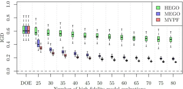
For this example, the results are arranged similar to the previous ones and are shown in Figure 11.

Figure 11: History of 50 independent runs of each proposed algorithm for the car-side impact optimization problem.

Again, of the three Kriging-based strategies, MVPF presented, in all iterations, the lowest values for the IGD criterion. The final IGD results for the three techniques are: MVPF = 0.1340±0.006, MEGO = 0.191±0.01 and HEGO = 0.464±0.05.

4.4 Integrating ‘moko’ with an external application

The greatest justification of using ‘moko’ (or any surrogate-based optimization algorithm) is to reduce computational cost when running complex optimization tasks. Indeed, the examples provided in this article would be optimized much faster by using a state-of-the-art multi-objective algorithm such as NSGA-II or SPEA-2 directly on the analytical functions. However, when the run time of a single call of a single objective or constraint is about several seconds or even minutes the number of required calls used by those algorithms makes the process unfeasible. This subsection aims to provide a small guidance for those who want to integrate ‘moko’ with an external application. The core function used for this is the base R ‘system’ function. This function invokes the operational system (OS) command specified by the ‘command’ field. The following example shows how this function could be used to call ANSYS Composite PrepPost:

system('”C:/Program Files/ANSYS Inc/v170/ACP/ACP.exe” --batch=1 C:/scripts/scriptfile.py')

In this example, the ANSYS executable is located on the folder “C:/Program Files/ANSYS Inc/v170/ACP”. The guidelines on how to execute the structural simulation are contained on a script file called “scriptfile.py” on the directory “C:/scripts”. How to create scripts for structural simulations on ANSYS is out of the scope of this paper, but the reader can find plenty of information on the internet and product manuals.

Since most computer aided engineering (CAE) software do not provide an application programming interface (API) to communicate with external tools, the easiest way to do this task is by the usage of plain text files (‘.txt’) or even comma separated files (‘.csv’). In R programming, this can be done with the commands ‘read.table’ and ‘write.table’.

5 FUTURE IMPLEMENTATIONS AND CONTRIBUTIONS

As ‘moko’ is an open source package, the interested reader is encouraged to look inside the code, test for bugs, request new features and even modify the code freely. The authors use the github2 _{platform to interface with the}

users of ‘moko’. There, anyone can chat with the developer, report bugs, and request for pulls of updated custom code.

There are some future implementations the authors plan adding to the package, which are listed in the following:

1. Entropy based infill criterion; 2. Informational based infill criterion; 3. KKTPM optimality criteria;

4. Efficient many-objective optimization (more than 4 objectives); 5. Efficient highly constrained optimization (small feasible space).

6 CONCLUDING REMARKS

In this paper, three Kriging based multi-objective optimization techniques are described (MEGO, HEGO and MVPF). The corresponding implementations can be found in the moko package, available on the CRAN servers at https://CRAN.R-project.org/package=moko. Three test problems were presented here: the Binh and Korn, the Nowacki beam and a side-car impact problems. These problems are based on analytical functions, the first two ones with two design variables and two objectives, and the later with three objectives, ten constraints and seven design variables. The first problem (Binh and Korn) has two constrains while the Nowacki beam has five. Even though the present paper uses analytical functions to demonstrate the usage of ‘moko’, the package is aimed to be employed for costly optimization tasks such as finite element and/or fluid dynamics simulations. In terms of high-fidelity model calls, all methods showed to be much more efficient than the direct NSGA-II algorithm. Of the three multi-objective optimization techniques, MVPF significantly outperformed the other two in the cases studied in this paper. The advantages of MVPF showed to be substantial in both performance (IGD mean) and robustness (IGD standard deviation). In addition, the authors reckon R language is a powerful easy-to implement and easy-to-use open source platform for numerical optimization.

References

Beume, N., Naujoks, B., and Emmerich, M. (2007). SMS-EMOA: Multiobjective selection based on dominated hypervolume. European Journal of Operational Research, 181(3):1653–1669.

Binh, T. T. and Korn, U. (1997). MOBES: A multiobjective evolution strategy for constrained optimization problems. In The Third International Conference on Genetic Algorithms (Mendel 97), volume 25, page 27.

Binois, M. and Picheny, V. (2016). GPareto: Gaussian Processes for Pareto Front Estimation and Optimization. R package version 1.0.2.

Carnell, R. (2012). LHS: Latin Hypercube Samples. R package version 0.10.

Chen, B., Zeng, W., Lin, Y., and Zhang, D. (2015). A new local search-based multiobjective optimization algorithm. Evolutionary Computation, IEEE Transactions on, 19(1):50–73.

Corne, D. W., Jerram, N. R., Knowles, J. D., and Oates, M. J. (2001, July). PESA-II: Region-based selection in evolutionary multiobjective optimization. In Proceedings of the 3rd Annual Conference on Genetic and Evolutionary Computation (pp. 283-290). Morgan Kaufmann Publishers Inc.

Deb, K. (2014). Multi-objective optimization. In Search methodologies, pages 403–449. Springer.

Deb, K., Pratap, A., Agarwal, S., and Meyarivan, T. (2002a). A fast and elitist multiobjective genetic algorithm: NSGA-II. Evolutionary Computation, IEEE Transactions on evolutionary computation, 6(2):182–197.

Deb, K., Thiele, L., Laumanns, M., and Zitzler, E. (2002b). Scalable multi-objective optimization test problems. In Evolutionary Computation, 2002. CEC’02. Proceedings of the 2002 Congress, volume 1, pages 825–830. IEEE.

Forrester, A., Sobester, A., and Keane, A. (2008). Engineering design via surrogate modelling: a practical guide. John Wiley & Sons, Pondicherry, India.

Ginsbourger, D., Picheny, V., Roustant, O., with contributions by Clément Chevalier, and Wagner, T. (2013). DiceOptim: Kriging-based optimization for computer experiments. R package version 1.4.

Jain, H., and Deb, K. (2014). An Evolutionary Many-Objective Optimization Algorithm Using Reference-Point Based Nondominated Sorting Approach, Part II: Handling Constraints and Extending to an Adaptive Approach. IEEE Trans. Evolutionary Computation, 18(4), 602-622.

Jones, D. R., Schonlau, M., and Welch, W. J. (1998). Efficient global optimization of expensive black-box functions. Journal of Global Optimization, 13(4):455–492.

Knowles, J. (2006). ParEGO: A hybrid algorithm with on-line landscape approximation for expensive multiobjective optimization problems. Evolutionary Computation, IEEE Transactions on, 10(1):50–66.

Krieg, D. (1951). A statistical approach to some basic mine valuation problems on the Witwatersrand. Journal of Chemical, Metallurgical, and Mining Society of South Africa, 52(6): 119-139.

Mersmann, O. MCO: Multiple Criteria Optimization Algorithms and Related Functions, 2014. R package version, 1.0.

Miettinen, K., and Mäkelä, M. M. (2002). On scalarizing functions in multiobjective optimization. OR spectrum, 24(2), 193-213.

Nikulin, Y., Miettinen, K., and Mäkelä, M. M. (2012). A new achievement scalarizing function based on parameterization in multiobjective optimization. OR spectrum, 34(1), 69-87.

Nowacki, H. (1980). Modelling of design decisions for CAD. In Computer Aided Design Modelling, Systems Engineering, CAD-Systems, pages 177–223. Springer.

Passos, A. G. and Luersen, M. A. (2016). Kriging-Based Multiobjective Optimization of a Fuselage-Like Composite Section with Curvilinear Fibers. In EngOpt 2016 - 5th International Conference on Engineering Optimization, Iguassu Falls, Brazil.

Passos, A. G. and Luersen, M. A. (2017b). MOKO: An Open Source Package for Multi-Objective Optimization with Kriging Surrogates. In MecSol 2017 - 6th International Symposium on Solid Mechanics, Joinville, Brazil. R package version 1.0-15.1.

Passos, A. G., and Luersen, M. A. (2018). Multiobjective optimization of laminated composite parts with curvilinear fibers using Kriging-based approaches. Structural and Multidisciplinary Optimization, 57(3), 1115-1127.

Roustant, O., Ginsbourger, D., and Deville, Y. (2012). DiceKriging, DiceOptim: Two R Packages for the Analysis of Computer Experiments by Kriging-Based Metamodeling and Optimization. Journal of Statistical Software, 51(1):1– 55.

Ruiz, A. B., Saborido, R., and Luque, M. (2015). A preference-based evolutionary algorithm for multiobjective optimization: the weighting achievement scalarizing function genetic algorithm. Journal of Global Optimization, 62(1), 101-129.

Sacks, J.; Welch, W. J.; Mitchell, T. J.; Wynn, H. P. (1989). Design and analysis of computer experiments. Statistical science, JSTOR, p. 409–423.

Scheuerer, M.; Schaback, R.; Schlather, M. (2013). Interpolation of spatial data a stochastic or a deterministic problem? European Journal of Applied Mathematics, 24(4), 601-629.

Shimoyama, K., Jeong, S., and Obayashi, S. (2013). Kriging-surrogate-based optimization considering expected hypervolume improvement in non-constrained many-objective test problems. In Evolutionary Computation (CEC), 2013 IEEE Congress on, pages 658–665. IEEE.

Srinivas, N. and Deb, K. (1994). Multi-Objective function optimization using non-dominated sorting genetic algorithms, Evolutionary Computation, 2(3), 221–248.

Van Veldhuizen, D. A. and Lamont, G. B. (1998). Multiobjective evolutionary algorithm research: A history and analysis. Technical report, Citeseer.

Wickham, H. (2015). R packages. O’Reilly Media, Inc.

Xiang, Y., Gubian, S., Suomela, B., and Hoeng, J. (2013). Generalized simulated annealing for global optimization: the GenSA Package. The R Journal, 5(1):13–29.

Zitzler, E. (1999). Evolutionary algorithms for multiobjective optimization: Methods and applications. Ph.D. thesis, Swiss Federal Institute of Technology Zurich.

Zitzler, E. and Thiele, L. (1998). Multiobjective optimization using evolutionary algorithms – a comparative case study. In Parallel problem solving from nature, pages 292–301. Springer.