Towards an online-coupled chemistry-climate model: evaluation of COSMO-ART

(1)

GMDD

4, 1809–1874, 2011

COSMO-ART evaluation

C. Knote et al.

Title Page

Abstract Introduction

Conclusions References

Tables Figures

◭ ◮

Back Close

Full Screen / Esc

Printer-friendly Version Interactive Discussion

Discussion

P

a

per

|

Dis

cussion

P

a

per

|

Discussion

P

a

per

|

Discussio

n

P

a

per

|

Geosci. Model Dev. Discuss., 4, 1809–1874, 2011 www.geosci-model-dev-discuss.net/4/1809/2011/ doi:10.5194/gmdd-4-1809-2011

Geoscientific Model Development Discussions

This discussion paper is/has been under review for the journal Geoscientific Model Development (GMD). Please refer to the corresponding final paper in GMD if available.

Towards an online-coupled

chemistry-climate model: evaluation of

COSMO-ART

C. Knote1,2, D. Brunner1,2, H. Vogel3, J. Allan4, A. Asmi5, M. Äij äl ä5, S. Carbone6, H. D. van der Gon7, J. L. Jimenez8, A. Kiendler-Scharr9, C. Mohr10, L. Poulain11, A. S. H. Pr év ôt10, E. Swietlicki12, and B. Vogel3

1

Laboratory for Air Pollution/Env. Technology, Empa Materials and Science, 8600 Duebendorf, Switzerland

2

C₂SM Center for Climate Systems Modeling, ETH, Zurich, Switzerland

3

Institute for Meteorology and Climate Research, Karlsruhe Institute of Technology, Karlsruhe, Germany

4

School of Earth Atmospheric, and Environmental Sciences, National Centre for Atmospheric Science, University of Manchester, Manchester, UK

5

Department of Physics, University of Helsinki, Helsinki, Finland

6

Air Quality Research, Finnish Meteorological Institute, Helsinki, Finland

7

TNO Princetonlaan 6, 3584 CB Utrecht, The Netherlands

8

(2)

GMDD

4, 1809–1874, 2011

C. Knote et al.

Title Page

Tables Figures

◭ ◮

Back Close

Full Screen / Esc

Discussion

P

a

per

|

Dis

cussion

P

a

per

|

Discussion

P

a

per

|

Discussio

n

P

a

per

|

9

Institut IEK-8, Troposph äre, Forschungszentrum J ülich, J ülich, Germany

10

Laboratory of Atmospheric Chemistry, Paul Scherrer Institute, Villigen, Switzerland

11

Leibniz Institute for Tropospheric Research, Leipzig, Germany

12

Division of Nuclear Physics, Department of Physics, Lund University, Lund, Sweden

Received: 9 July 2011 – Accepted: 25 July 2011 – Published: 4 August 2011

Correspondence to: D. Brunner (dominik.brunner@empa.ch)

(3)

GMDD

4, 1809–1874, 2011

C. Knote et al.

Title Page

Tables Figures

◭ ◮

Back Close

Full Screen / Esc

Discussion

P

a

per

|

Dis

cussion

P

a

per

|

Discussion

P

a

per

|

Discussio

n

P

a

per

|

Abstract

The online-coupled, regional chemistry transport model COSMO-ART is evaluated for periods in all seasons against several measurement datasets to assess its ability to rep-resent gaseous pollutants and ambient aerosol characteristics over the European do-main. Measurements used in the comparison include long-term station observations, 5

satellite and ground-based remote sensing products, and complex datasets of aerosol chemical composition and number size distribution from recent field campaigns. This is the first time these comprehensive measurements of aerosol characteristics in Europe are used to evaluate a regional chemistry transport model. We show a detailed analy-sis of the simulated size-resolved chemical composition under different meteorological 10

conditions. The model is able to represent trace gas concentrations with good accu-racy and reproduces bulk aerosol properties rather well though with a clear tendency to underestimate both total mass (PM10 and PM2.5) and aerosol optical depth. We

find indications of an overestimation of shipping emissions. Time evolution of aerosol chemical composition is captured, although some biases are found in relative com-15

position. Nitrate aerosol components are on average overestimated, and sulfates un-derestimated. The accuracy of simulated organics depends strongly on season and location. While strongly underestimated during summer, organic mass is comparable in spring and autumn. We see indications for an overestimated fractional contribution of primary organic matter in urban areas and an underestimation of SOA at many lo-20

(4)

GMDD

4, 1809–1874, 2011

C. Knote et al.

Title Page

Tables Figures

◭ ◮

Back Close

Full Screen / Esc

Discussion

P

a

per

|

Dis

cussion

P

a

per

|

Discussion

P

a

per

|

Discussio

n

P

a

per

|

1 Introduction

Aerosols affect climate through changes in the radiation budget (direct effect), the subsequent changes in atmospheric stratification (semi-direct effect, Haywood and Boucher, 2000) and through changes in cloud development and lifetime due to the differences in available cloud condensation/ice nuclei (indirect effects, Lohmann and 5

Feichter, 2005). Aerosols also constitute a health concern if they are small enough to traverse the human respiratory tract (Laden et al., 2006; Dockery et al., 1996). Once in the lungs their toxicity depends on size (Donaldson et al., 2000) and chemical composi-tion (Aktories et al., 2009; Hoek et al., 2002). Within the climate system, their influence on the radiation budget depends on their optical properties, and how they affect clouds 10

is a function of size and hygroscopicity. Size, chemical composition, and optical prop-erties are therefore indispensable parameters that need to be well represented if any study of aerosol effects should be accurate.

Up to now, climate modeling studies including aerosols often lack a comprehensive description of aerosol characteristics, due to the high computational demand of such 15

a complex effort. Approaches range from simple bulk mass aerosol schemes with only externally mixed aerosols, up to multi-component, size-resolving aerosol modules including explicit aging of aerosols and interactions with radiation and clouds. Often these modules lack parts (or all) of the interaction between gas- and aerosol-phase. Nucleation of ammonium-sulfate particles is represented in most models, and also 20

the condensation of organics onto particles is included in some. Nitrates, which can represent up to 50 % of ambient aerosol mass in polluted regions (Putaud et al., 2004), were missing for example in all but two models participating in the Fourth Assessment Report of the Intergovernmental Panel on Climate Change (IPCC, Meehl et al., 2007). This was probably due to the lack of the necessary, but computationally expensive, 25

gas-phase chemistry leading to nitrate formation.

(5)

GMDD

4, 1809–1874, 2011

C. Knote et al.

Title Page

Tables Figures

◭ ◮

Back Close

Full Screen / Esc

Discussion

P

a

per

|

Dis

cussion

P

a

per

|

Discussion

P

a

per

|

Discussio

n

P

a

per

|

it is necessary to couple climate and air quality models. One such modeling system which focuses on the regional scale combines the numerical weather prediction model of the Consortium for Small Scale Modeling (COSMO, Baldauf et al., 2011) with an extension for Aerosols and Reactive Trace gases: COSMO-ART (Vogel et al., 2009). It is based on state-of-the-art components for the description of meteorology, chemistry 5

and aerosols and features an integrated approach to couple them. Such an “online”-coupling allows for consistent treatment of all components by the same parameteriza-tion (e.g. advecparameteriza-tion, diffusion, convection) and avoids unnecessary interpolation steps. Additionally, simulation of feedbacks between chemistry, aerosols and meteorology be-comes possible. Grell and Baklanov (2011) showed the importance of this approach 10

and its benefits compared to traditional “o_ffline” models, and Zhang (2008) gave a com-prehensive overview of the available modeling systems. COSMO-ART is in its compo-sition very similar to the Weather Research and Forecasting model (WRF) extended by chemistry and aerosols: WRF/chem. Grell et al. (2005) presented a comprehensive evaluation for this modeling system. Most of the components of COSMO-ART are well 15

known and tested. However, their interplay and integration into the modeling system lacks a thorough evaluation.

In this work we analyse COSMO-ART regarding its ability to represent ambient con-centrations of gaseous and particulate matter constituents over Europe under diff er-ent meteorological conditions. Particular focus is laid on the accuracy of the repre-20

sentation of climate relevant parameters of aerosols, i.e. their optical properties and ability to act as cloud condensation nuclei. We have collected an extensive eval-uation dataset of satellite-derived NO₂ and aerosol optical depth (AOD), long-term station measurements for gas-phase tracers, bulk aerosol mass and optical proper-ties, as well as aerosol mass spectrometer (AMS) measurements of aerosol chemi-25

(6)

GMDD

4, 1809–1874, 2011

C. Knote et al.

Title Page

Tables Figures

◭ ◮

Back Close

Full Screen / Esc

Discussion

P

a

per

|

Dis

cussion

P

a

per

|

Discussion

P

a

per

|

Discussio

n

P

a

per

|

European Monitoring and Evaluation Programme (EMEP, http://www.emep.int) and in coordinated measurements of the European Supersites for Atmospheric Aerosol Re-search (EUSAAR, http://www.eusaar.net) and the German Ultrafine Aerosol Network (GUAN, Birmili et al., 2009).

Our simulations employ full gas-phase chemistry and aerosol dynamics. Spatial and 5

temporal resolution of input data (meteorology, anthropogenic emissions) and model setup is on the top end of currently possible simulations. While the modeling system is currently still too expensive to be used for climate simulations, the results of our evaluation efforts can be seen as a benchmark for what degree of accuracy can be expected in future fully-coupled regional chemistry-climate models, and identify model 10

deficiencies which would need to be remedied before such simulations can be made. We begin with a description of the system, its setup and the measurement datasets used in evaluation. The second chapter describes the findings of our evaluation against the di_fferent datasets and discusses the results. The last chapter provides a more in-depth discussion of simulated aerosol characteristics. We conclude with implications 15

for future studies and give directions for further developments of the modeling system.

2 Methods

2.1 Modeling system

COSMO-ART is a regional chemistry transport model, online-coupled to the COSMO regional numerical weather prediction and climate model (Baldauf et al., 2011). 20

COSMO is operationally used for numerical weather prediction (NWP) purposes by several European national meteorological services and research institutes. In its mate version (Rockel et al., 2008) it has been used in several studies of regional cli-mate impact assessment (e.g. Jaeger and Seneviratne, 2010; Suklitsch et al., 2008; Hohenegger et al., 2008) and participated in the IPCC fourth assessment report mod-25

(7)

GMDD

4, 1809–1874, 2011

C. Knote et al.

Title Page

Tables Figures

◭ ◮

Back Close

Full Screen / Esc

Discussion

P

a

per

|

Dis

cussion

P

a

per

|

Discussion

P

a

per

|

Discussio

n

P

a

per

|

Trace gases (ART) contains a modified version of the Regional Acid Deposition Model, Version 2 (RADM2) gas-phase chemistry mechanism (Stockwell et al., 1990). It has been extended by a more sophisticated isoprene scheme of Geiger et al. (2003) for a better description of biogenic volatile organic compounds (VOC), but does not include recent findings regarding formation of secondary organic aerosols and OH recycling 5

due to isoprene chemistry (e.g. Paulot et al., 2009). Aerosols are represented by the modal aerosol module MADE (Modal Aerosol Dynamics Model for Europe, Ackermann et al., 1998), improved by explicit treatment of soot aging through condensation of inor-ganic salts (Riemer et al., 2003) and additional modes for mineral dust (Stanelle et al., 2010) and sea salt. Nucleation of new particles is formulated according to Kerminen 10

and Wexler (1994) allowing for binary homogeneous nucleation of sulfuric acid. The condensation of vapours from biogenic and anthropogenic VOCs is parametrized with the Secondary Organic Aerosol Model (SORGAM) of Schell et al. (2001). This is still a commonly used module, although Fast et al. (2009) showed that this scheme under-predicts SOA concentrations up to a factor of 10 in very polluted regions. Biogenic VOC 15

emission fluxes, considering isoprene,α-pinene, other monoterpenes and a class of unidentified compounds, are calculated online with a Guenther-type model presented in Vogel et al. (1995), using land use data from the Global Land Cover 2000 (GLC2000) dataset (Bartholom ´e and Belward, 2005). Seasalt emissions follow Lundgren (2006), and mineral dust is parameterized as described in Vogel et al. (2006). Dry deposition 20

is modeled by a resistance approach (Baer and Nester, 1992). Washout of aerosols is included by a parameterization of Rinke (2008). Wet removal of gases and aqueous-phase chemistry are currently not considered. COSMO-ART is fully online-coupled, and currently allows for feedbacks of aerosols on radiation (direct / semi-indirect ef-fects). Cloud feedbacks (indirect effects) have been included in a research version 25

(8)

GMDD

4, 1809–1874, 2011

C. Knote et al.

Title Page

Tables Figures

◭ ◮

Back Close

Full Screen / Esc

Discussion

P

a

per

|

Dis

cussion

P

a

per

|

Discussion

P

a

per

|

Discussio

n

P

a

per

|

For meteorology we used initial and boundary conditions from the European Cen-tre for Medium-Range Weather Forecasts (ECMWF) Integrated Forecast System (IFS) model, with an update frequency of 3 h. Boundary data for gas-phase species, includ-ing most of the lumped NMVOC compounds, were provided through simulations of the Model for Ozone and Related chemical Tracers (MOZART) driven by meteorological 5

data from the National Center for Environmental Prediction (NCEP) presented in Em-mons et al. (2010), with an update frequency of 6 h. No boundary data for aerosol components were available from MOZART or other models that matched our aerosol mechanism. Therefore, we took the output of a previous (otherwise identical) simula-tion of COSMO-ART and chose one point in the Northern Atlantic (8.7◦_{W, 47.4}◦_{N, see}

10

Fig. 1). We averaged the simulated aerosol characteristics over the complete simula-tion period, and used this vertical column as lateral boundary condisimula-tions for all aerosol variables. While this gives more realistic aerosol concentrations at the boundaries, the total inflow will still be underestimated.

The emission inventory for Europe developed by TNO (Netherlands) within the Mon-15

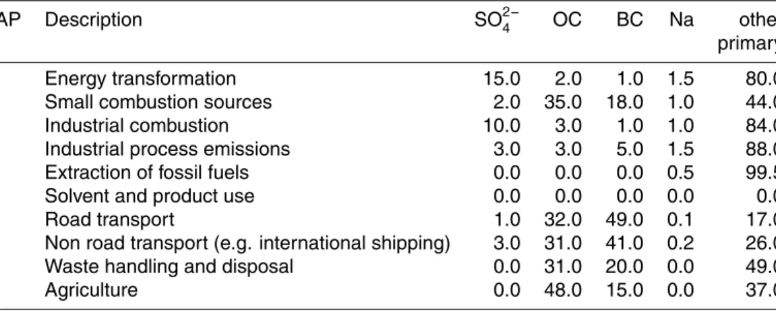
itoring Atmospheric Composition and Climate (MACC) project (TNO/MACC, Kuenen et al., 2011; Denier van der Gon et al., 2010) provides anthropogenic emissions. This is a follow-up and improvement of the earlier TNO-GEMS emission database (Viss-chedijk et al., 2007). Therein, emissions from 10 different SNAP (Selected Nomencla-ture for sources of Air Pollution) source categories are represented by a spatial pattern 20

of annual emission totals for the years 2003–2007, and statistical time functions for species, country and source category dependent monthly, weekly and daily cycles. Our speciation of non-methane volatile organic compounds (NMVOC) mass totals is done using composition information from Passant (2002) and a translation matrix to RADM2 (J. Keller, PSI, Switzerland, personal communication, 2009). Aerosol emis-25

sions are provided as mass totals of particulate matter below 10 µm (PM₁₀) and below 2.5 µm (PM2.5) in diameter. We distribute them onto the different MADE modes

(9)

GMDD

4, 1809–1874, 2011

C. Knote et al.

Title Page

Tables Figures

◭ ◮

Back Close

Full Screen / Esc

Discussion

P

a

per

|

Dis

cussion

P

a

per

|

Discussion

P

a

per

|

Discussio

n

P

a

per

|

International Institute for Applied Systems Analysis (IIASA, PRIMES09 scenario) serve to extrapolate TNO/MACC emissions to years after 2007. With its spatial resolution of about 8 km (0.125×0.0625◦), the description of the time evolution of emissions and the comprehensive set of emitted species this dataset is one of the most detailed cur-rently available emission inventories for Europe. Preparation of all input datasets for 5

COSMO-ART is done using INT2COSMO-ART (Appendix A).

Our modeling domain (Fig. 1) covers the greater European region, with a horizontal resolution of 0.17◦ _{and a grid of 200}

×190 points. Vertically, the model is discretized into 40 terrain-following hybrid sigma levels, with the lowest level at 10 m and ranging up to approx. 24 000 m (20 hPa). A Runge-Kutta time integration scheme is employed 10

with time steps of 40 s. Tracers are advected horizontally via a semi-lagrangian method conserving mass over the total domain (“globally mass-conserving”). The overall model configuration closely follows the current operational setup of COSMO-EU of the Ger-man Meteorological Service (DWD).

2.2 Measurement data

15

Meteorological parameters have been taken from the operational surface synoptic ob-servations (SYNOP) network, providing measurements for temperature, dew point tem-perature, wind speed and direction at or in the vicinity of most measurement points of chemical composition. In the EMEP programme a number of stations through-out Europe report quality-controlled, long-term measurements of gaseous precur-20

sor substances and aerosol variables. AIRBASE (European AIR quality dataBASE, http://airbase.eionet.europa.eu/) data provides measurements at a much larger num-ber of stations, but with heterogeneous quality and mostly at rather polluted locations not representative for the model grid size of 0.17◦_{(approx. 19 km at model domain}

cen-ter). While AIRBASE, in its recently published version 5, provides data up to the end of 25

(10)

GMDD

4, 1809–1874, 2011

C. Knote et al.

Title Page

Tables Figures

◭ ◮

Back Close

Full Screen / Esc

Discussion

P

a

per

|

Dis

cussion

P

a

per

|

Discussion

P

a

per

|

Discussio

n

P

a

per

|

from AIRBASE, but restricted the stations used to those which also report to EMEP. As discrepancies between modelled and measured values might be reasoned by the type and location of a measurement station, we have additionally disaggregated the se-lected stations into categories based on the representativeness study done by Henne et al. (2010), which includes a more comprehensive analysis of the surroundings of 5

each station. Therein, stations are classified regarding their pollution burden and us-ability in a model evaluation. We have used the “alternative classification” described in the Supplement S3 in Henne et al. (2010), which gives classes ranging from very clean stations (“rural/remote”), via stations with very variable pollution levels (“rural/coastal”) and stations representative for a larger area (“rural”), up to stations with a strong influ-10

ence of large urban areas in their vincinity (“suburban/urban”). Most EMEP stations are found in the “rural” and “rural/coastal” classes, and are seen as the most representative when evaluating model results.

The Aerosol Robotic Network (AERONET) (Holben et al., 1998) provides measure-ments of aerosol optical depth (AOD) for analysis of the optical properties. Aerosol 15

mass spectrometer (AMS) measurements give quantitative measurements of the chemical composition of submicron non-refractory aerosol mass (NR−PM1) with high

temporal resolution (Canagaratna et al., 2007). AMS data collected at several sites throughout Europe during measurement campaigns of the EMEP/EUCAARI project in October 2008 and March 2009 were used, as well as from an EMEP intensive cam-20

paign in June 2006. Homogenized measurements of aerosol size distribution from scanning mobility particle sizer (SMPS) and differential mobility particle sizer (DMPS) instruments were provided in Asmi et al. (2011) as a result of the EUSAAR project and data from the GUAN network (Birmili et al., 2009), with 24 measurement sites in Europe. Figure 1 shows the locations of ground-based stations used in our evaluation. 25

Finally, satellite-derived datasets provide a vertically integrated view on model per-formance. In our analysis, tropospheric columns of NO2 from the Ozone Monitoring

Instrument (OMI) were used for gas-phase comparison. The NO2columns are based

(11)

GMDD

4, 1809–1874, 2011

C. Knote et al.

Title Page

Tables Figures

◭ ◮

Back Close

Full Screen / Esc

Discussion

P

a

per

|

Dis

cussion

P

a

per

|

Discussion

P

a

per

|

Discussio

n

P

a

per

|

compared to operational products in particular regarding a better representation of topography and surface reflectance using high-resolution data sets (Zhou et al., 2009, 2010). To estimate the accuracy of the spatial distribution of simulated aerosol loadings aerosol optical depth (AOD) retrieved from the Moderate Resolution Imaging Spectrom-eter (MODIS) (Levy et al., 2007, MOD04 L2 product) were used.

5

2.3 Investigation periods

The selection of the investigation periods was driven by two goals: to evaluate model performance under typical weather conditions and in all seasons, and to have AMS measurement data available for comparison. Apart from the campaign measurement data, AIRBASE and satellite data were available for all simulations. The following peri-10

ods were chosen:

2.3.1 “Winter case”: 23 January–11 February 2006

A stable high pressure system with very low surface temperatures was present over Europe from 23 January onwards, with only minor disturbances on 5–7 February. Over Switzerland and Eastern Europe, this resulted in an episode with strong temperature 15

inversions and exceptionally high particulate matter (PM) concentrations. The Swiss legislative limit for daily mean PM10 (particulate matter below 10 µm in diameter) of

50 µg m−3 _{was exceeded every day between 27 January and 5 February at several}

measurement stations. This episode represents a typical winter situation where high pollution levels are building up through strong inversions and local emissions are the 20

strongest contributors to pollution levels (Holst et al., 2008).

2.3.2 “Summer case”: 10–29 June 2006

(12)

GMDD

4, 1809–1874, 2011

C. Knote et al.

Title Page

Tables Figures

◭ ◮

Back Close

Full Screen / Esc

Discussion

P

a

per

|

Dis

cussion

P

a

per

|

Discussion

P

a

per

|

Discussio

n

P

a

per

|

thunderstorms on 25 to 29 June. Such a situation is associated with strong photo-chemistry and high O3 levels, representing a typical “summersmog” episode. AMS

instruments were deployed in Payerne (CH), Harwell and Auchencorth (UK) during this period in the context of an EMEP intensive measurement campaign.

2.3.3 “Autumn case”: 1–20 October 2008

5

A low pressure system over Scandinavia brought polar airmasses towards Europe at the beginning of the month. From 5–20 October generally mild and sunny conditions prevailed. On 16 October a low pressure disturbance passed, bringing rain to Central Europe. Frequent disturbances by mesoscale systems gradually change a summer-time atmosphere towards a wintersummer-time one in this simulation. During this period, an 10

EMEP/EUCAARI measurement campaign took place, from which we received AMS data for Payerne (CH), Melpitz (DE), Vavihill (SE), Hyyti ¨al ¨a (FI) and K-Puszta (HU). EUSAAR size distribution data were available for this period.

2.3.4 “Spring case”: 1–20 March 2009

A low pressure system originating over the North Atlantic brought cold weather on 15

1 and 2 March. It was followed by spring-like conditions from 13–18 March, and a cold surge from NE on 20 March. We regard this situation as typically spring-like, with first warm days including the initial onset of BVOC emissions, intermitted by “cleansing” periods with clouds, precipitation and strong mesoscale forcing. An-other EMEP/EUCAARI campaign took place during this period, from which we present 20

(13)

GMDD

4, 1809–1874, 2011

C. Knote et al.

Title Page

Tables Figures

◭ ◮

Back Close

Full Screen / Esc

Discussion

P

a

per

|

Dis

cussion

P

a

per

|

Discussion

P

a

per

|

Discussio

n

P

a

per

|

3 Evaluation

3.1 Meteorology

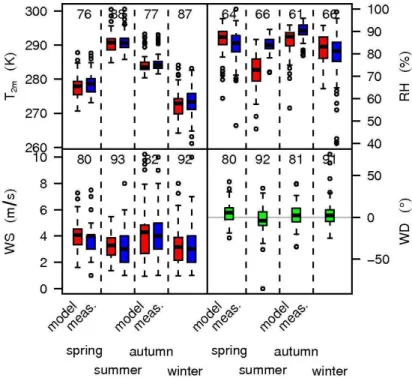
In all periods, the comparison of simulated temperature, dew point temperature, wind direction and wind speed show very good agreement with SYNOP measurement data both in terms of temporal variability and average values (Fig. 2). Sometimes the (di-5

urnal) variability is underestimated by the simulations (not shown), which is not unex-pected for such coarse grid simulations due to the averaging onto a 0.17◦ _{grid box}

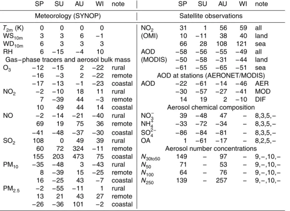
(e.g. Schl ¨unzen and Katzfey, 2003; Heinemann and Kerschgens, 2005). The means of temperature, wind speed and direction are well reproduced (Table 2). Except for the summer 2006 period, where the model shows a negative bias (Fig. 2), also relative 10

humidity is realistically represented. The negative bias in summer 2006 might be rea-soned by an unrealistic initialization of soil moisture. Further investigation is needed to remedy this deficiency.

IFS analysis data was used to initialize and force the model at the lateral boundaries. Within the model domain COSMO runs freely, creating its own dynamics. This is not 15

the best possible setup. Constant data assimilation from observations like it is done for operational analysis (e.g. nudging), or a reinitialization of meteorology after one or two days could further improve meteorology. However, we found no significant loss in ac-curacy of the simulation over the whole integration period when compared against sev-eral SYNOP stations, suggesting that the latsev-eral forcing provides a sufficiently strong 20

constraint for the meteorology within the model domain. Some of the underestimated (diurnal) variability found would likely be improved at increased resolution.

The modest deficiencies found such as an underestimated diurnal variability are well known to NWP modellers and represent problems such models are currently faced with in general. Mean wind speeds simulated by the model, for example, are below 5 % 25

(14)

GMDD

4, 1809–1874, 2011

C. Knote et al.

Title Page

Tables Figures

◭ ◮

Back Close

Full Screen / Esc

Discussion

P

a

per

|

Dis

cussion

P

a

per

|

Discussion

P

a

per

|

Discussio

n

P

a

per

|

a successful air quality simulation. They also highlight one of the key benefits of this modeling system: its direct coupling to an operational weather prediction model.

3.2 Gas-phase

3.2.1 Mean concentrations

We have calculated the distribution of median pollutant concentrations at all stations in 5

the model domain over each simulation period. Shown in Figure 3 are the distributions of O₃, NO₂, NO, SO₂, PM₁₀and PM₂_.₅for different station classes. They are presented by boxplots of the distribution of measured and modelled median values during each season (afternoon values of hours 12:00–18:00 LT) and allow to evaluate accuracy and potentially existing biases in our simulations. Table 2 gives a summary of the mean 10

biases found.

O3 is the measure air quality models often have been “tuned” for. COSMO-ART is

no different from other models in its ability to represent this quantity very well. A small but consistent underestimation is visible, but seasonal di_fferences are well captured. In winter 2006 largest (negative) biases are observed, while autumn 2008 matches mea-15

surements best (Table 2). Overall biases in the median never exceed 10 ppbv and are often below 5 ppbv. Variability within the distributions is comparable with observations. Overall, a correlation of 0.7 (r) with hourly station values shows that the performance of our O3simulations are in the same range as results from simulations with comparable

modeling systems like WRF/Chem in Grell et al. (2005). 20

The O3 precursors NO and NO2 measured within the AIRBASE network show a

much larger variability than O3 itself. The differences between rural and rural/remote

stations in concentrations of NO and NO₂ are well reproduced by the model. Spring 2009, summer 2006 and autumn 2008 concentrations are in a similar range, while val-ues more than twice the median of the other seasons were measured during the high 25

(15)

GMDD

4, 1809–1874, 2011

C. Knote et al.

Title Page

Tables Figures

◭ ◮

Back Close

Full Screen / Esc

Discussion

P

a

per

|

Dis

cussion

P

a

per

|

Discussion

P

a

per

|

Discussio

n

P

a

per

|

represents. However, a comparably strong underestimation is found in summer 2006. Steinbacher et al. (2007) and Dunlea et al. (2007) showed that the often used molyb-denum converter based NO2measurements are biased high due to the additional

con-version of other oxidized nitrogen compounds. This will influence the comparison es-pecially during this period, which is characterized by the high oxidative capacity of the 5

atmosphere due to warm, sunny conditions. “Rural/coastal” stations show an overes-timation throughout all simulation periods (Table 2). In summary we conclude that the model is able to accurately simulate NO_x.

SO2levels are generally overestimated, especially at coastal stations. Only during

the summer 2006 period, “rural” stations compare well to modelled results. The in-10

crease in SO₂ concentrations during the polluted winter 2006 episode is reproduced, though exaggerated. We argue that a missing parameterization in COSMO-ART for wet scavenging of gases can explain a large part of this SO2overestimation. Also the

associated removal of SO₂by oxidation to particulate SO2−

4 within cloud droplets is not

yet implemented, further contributing to too high SO2levels. An overestimation of SO2

15

emissions in the TNO/MACC inventory could also be responsible for the observed mis-match. Uncertainties in emission inventories for SO₂have been shown to be generally large (de Meij et al., 2006), and even more so for their strongest contributor, interna-tional shipping (Endresen et al., 2005), consistent with the stronger overestimation at coastal stations. However, no other species shows a similar overestimation (over land) 20

in our simulations.

Very few measurements were available for NH3 (3 stations in the Netherlands). At

those points, NH3 levels are on average well represented, but show large variability

throughout the simulation period (not shown).

NMVOCs, the components missing to assess the tropospheric chemistry as a whole, 25

(16)

GMDD

4, 1809–1874, 2011

C. Knote et al.

Title Page

Tables Figures

◭ ◮

Back Close

Full Screen / Esc

Discussion

P

a

per

|

Dis

cussion

P

a

per

|

Discussion

P

a

per

|

Discussio

n

P

a

per

|

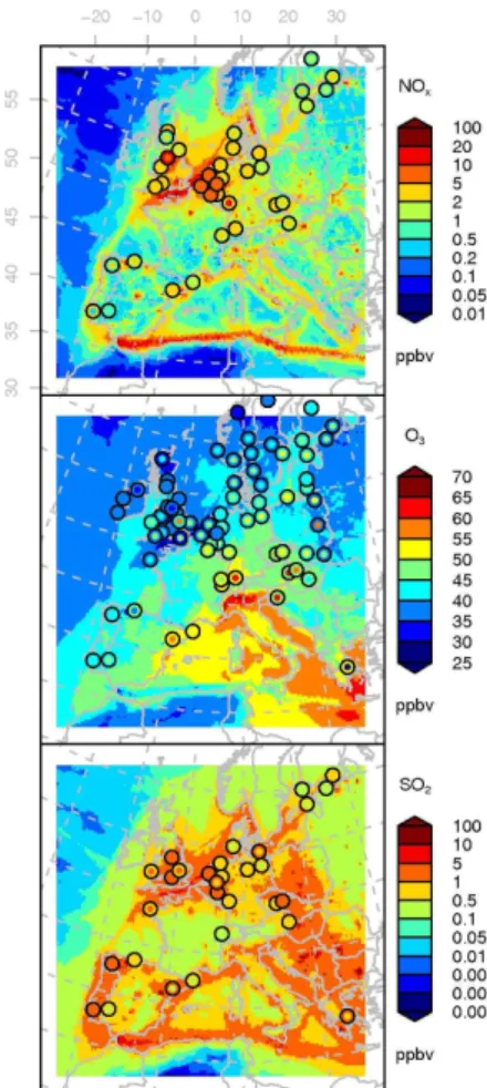
3.2.2 Spatial distribution

Maps of mean afternoon (hours 12:00–18:00 UTC) concentrations over the whole sim-ulation period were produced, overlaid with point indicators of the same mean concen-trations at each measurement station (Fig. 4 for summer 2006 and in the Supplement for the other periods).

5

The spatial distribution of O₃ and NO_x concentrations generally corresponds well with observed values. Only minor differences are found, as for example a large inter-station variability of measured O3 in Eastern Europe which is not seen in the model,

and an underestimation of O₃ concentrations over the Iberian Peninsula during the spring 2009 period. NO_x values show no region with exceptional biases over land. 10

Striking, however, are the high modelled values of NOx, but also of SO2, over water,

along shipping routes in the Mediterranean Sea and the English Channel. The general overestimation of SO₂ concentrations found in evaluation of the mean quantities is clearly visibile throughout Europe for the autumn 2008 period, but less so in the other periods. Modelled SO2concentrations at coastal stations in NE Spain are consistently

15

too high. Apart from that no distinct spatial pattern of overestimation could be found.

3.2.3 Diurnal cycles

The representation of the diurnal cycle of atmospheric constituents was evaluated by means of ensemble plots. The ensemble consisted of all stations which had measure-ment data for the compound of interest, disaggregated by the classification of Henne 20

et al. (2010). The distribution of concentrations was then calculated for each hour of day, over the whole simulation period. The median and the range covering 70 and 90 % of all stations are shown in Fig. 5 (see Supplement for plots of the other periods).

The simulated daily cycle of O3 is accurate throughout most seasons and station

types. The slight underestimation of mean O3concentrations found is visible as a shift

25

(17)

GMDD

4, 1809–1874, 2011

C. Knote et al.

Title Page

Tables Figures

◭ ◮

Back Close

Full Screen / Esc

Discussion

P

a

per

|

Dis

cussion

P

a

per

|

Discussion

P

a

per

|

Discussio

n

P

a

per

|

Simulated NO₂diurnal cycles also correspond well with observations in most cases. Important aspects like the peaks during morning and evening hours (“rush-hour”) vis-ible in the spring 2009 and autumn 2008 periods are reproduced. NO2 levels during

nighttime are overestimated in spring 2009 for rural stations, and in autumn 2008 for rural and rural/remote stations. This overestimation at night could be a consequence 5

of the fact that in reality the station is away from emission sources of NO2, though in

the model NO₂ is emitted directly into the grid box the station is located in. In spring 2009 (rural stations) and summer 2006 (rural and rural/remote), an exaggerated diur-nal amplitude leads to underestimations of NO2 concentrations during daytime. Here

again, the positive measurement bias will have an influence on our comparison with 10

high levels of oxidized nitrogen compounds such as peroxyacetylnitrates (PAN) and HNO3in the afternoon, leading to positive biases in the measured NO2concentrations

(Steinbacher et al., 2007; Dunlea et al., 2007). Simulated inter-station-type variability is comparable with measurements.

Nitric oxide compares well to observations during daytime, but is underestimated at 15

night. The relatively high measured concentrations at nighttime could be an indication for local sources a_ffecting the measurement sites since NO_x is mostly emitted in the form of NO and then rapidly converted to NO2by reaction with ozone. This

interpreta-tion is supported by the comparatively high NO:NO2ratios of the measurements. The

model, conversely, shows very low NO values as expected for truly remote sites (Car-20

roll et al., 1992; Brown et al., 2004). Overall the diurnal cycle with low values during nighttime, a distinct peak during morning hours and a slow reduction towards evening is captured accurately in all simulated periods.

Only 3 measurement points were available to investigate the simulation quality of NH3, and all were located in the (highly NH3loaded) Netherlands, making this

compar-25

(18)

GMDD

4, 1809–1874, 2011

C. Knote et al.

Title Page

Tables Figures

◭ ◮

Back Close

Full Screen / Esc

Discussion

P

a

per

|

Dis

cussion

P

a

per

|

Discussion

P

a

per

|

Discussio

n

P

a

per

|

activities, especially livestock and manure. NH3concentrations are mostly dominated

by local emissions. It is known that the diurnal cycle of NH₃emissions strongly depends on the emission source (Reidy et al., 2009). Ellis et al. (2011) showed that bi-directional fluxes between the atmosphere and land surfaces might be needed to accurately sim-ulate NH₃(and associated aerosol) levels. All this makes modeling such emissions a 5

major challenge which is currently not accurately addressed in most models (Zhang et al., 2008), as emission inventories based on spatially distributed emission totals and associated, statistically averaged time functions cannot capture such process-based emissions.

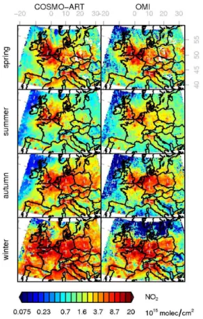
3.2.4 Satellite observations

10

For comparison with OMI satellite information, vertical tropospheric columns (VTCs) of NO₂were calculated from model output for the hour of the satellite overpass (13:30 LT, approx. 12:30 UTC over Europe). The height of the troposphere was assumed to be fixed over all simulations at 10 km geometric height, the exact choice has little influence on the NO₂columns. The comparison was made only where OMI data were available 15

at each overpass and the conditions were nearly cloud-free (cloud radiance fraction re-ported by OMI retrieval<50 %, corresponding to approx. <20 % cloud coverage). The arithmetic mean over each simulation period was calculated and the results are shown in Fig. 6. The aggregated mean biases for all grid points, land points and sea points can be found in Table 2. We compared the model simulated NO2columns directly with the

20

respective EOMINO columns without taking into account the averaging kernels which would remove the dependency of the result on the a priori NO2 profiles used in the

EOMINO retrieval. Not accounting for the averaging kernels might introduce biases of the order of 30 % with EOMINO columns tending to be too high over remote locations and too low over polluted areas (Russell et al., 2011), while differences averaged over 25

Europe are likely to be small (Huijnen et al., 2010).

Spatial distribution and magnitude of NO2compares well with our modeling results.

(19)

GMDD

4, 1809–1874, 2011

C. Knote et al.

Title Page

Tables Figures

◭ ◮

Back Close

Full Screen / Esc

Discussion

P

a

per

|

Dis

cussion

P

a

per

|

Discussion

P

a

per

|

Discussio

n

P

a

per

|

as the Po Valley (Italy) are accurately captured. Large urban agglomerations (Paris, Madrid, Berlin, Warszaw) are comparable in extent and magnitude. Also, cleaner re-gions like for example southern France are well represented. Notable differences are mostly found in polluted coastal areas, especially in the Mediterranean Sea, where the model tends to overestimate NO₂concentrations over water, particularly in the autumn 5

2008 and spring 2009 period. This overestimation is also visible in the mean over all grid points over sea in Table 2. Emission estimates for ship traffic are known to have large error margins both in magnitude (Corbett and Koehler, 2003) and spatial alloca-tion (Wang et al., 2008). From the magnitude of the error and the spatial correlaalloca-tion with main shipping routes an overestimation of ship emissions by the inventory used 10

is likely. This would also explain the consistent overestimation of SO₂ concentrations at coastal stations in NE Spain. Seasonal differences are nicely captured for spring, summer and autumn, only the model results for the winter 2006 period overestimate NO₂columns noteably in Northern and Eastern Europe.

3.3 Aerosol characteristics

15

All comparisons of measured and modelled particulate matter were made in an as rigorous as possible manner. For PM10 and PM2.5 bulk mass and NR−PM1 AMS

measurements, the modelled log-normal distribution functions were integrated over the respective size ranges, and size cut functions were employed to simulate the size-dependent transmission efficiency that is typically found in the measurement instru-20

ments used. See Appendix B for a description of the transmission functions used. For the AMS the modelled quantities were additionally converted to vacuum aerodynamic diameter (DeCarlo et al., 2004). No transmission functions were applied to number size distribution measurements, the modelled values are derived from integration over the exact intervals given: 30 to 50 nm, 50 to 500 nm, 100 to 500 nm and 250 to 500 nm, 25

(20)

GMDD

4, 1809–1874, 2011

C. Knote et al.

Title Page

Tables Figures

◭ ◮

Back Close

Full Screen / Esc

Discussion

P

a

per

|

Dis

cussion

P

a

per

|

Discussion

P

a

per

|

Discussio

n

P

a

per

|

3.3.1 Bulk mass

Continous bulk aerosol mass measurements are the least available within the measure-ment dataset, making the ensemble of stations for comparison very small (max. 8 sta-tions). When looking at PM₁₀ concentrations (Fig. 3, Table 2), our simulations match observations for rural stations in autumn 2008, and underestimate them in the other pe-5

riods. Simulated concentrations for rural/remote stations are almost identical to those at rural stations in the model, while in reality large differences are found. In conse-quence, modelled values are above measurements in spring 2009 and autumn 2008, but below in summer and winter 2006. Rural/coastal station concentrations are under-estimated in spring 2009 and summer 2006, match observations in autumn 2008 and 10

are above measurements in winter 2006. All this makes autumn 2008 the period in which PM10 is simulated best, and worst in summer 2006 (Table 2).

“Rural”-type stations are deemed the most representative for such a model evalu-ation, and they show (except in autumn 2008) an underestimation typical for many regional models (see e.g. Stern et al., 2008), probably due to missing sources (e.g. 15

resuspension, secondary organics, local mineral dust sources, missing aq.-phase con-version of SO₂ to SO2−

4 ). Stations of type “rural/coastal”, in contrast, have a

ten-dency towards more positive biases, which is reasoned by the high amounts of seasalt aerosols found at these stations in the modeling results. The overestimation could also be an artefact of the limited model resolution: coastal stations may be located in grid 20

cells partly covered by sea where sea salt aerosols are therefore emitted directly. Fur-ther investigations, e.g. comparisons with filter samples, are needed to assess if the amount of seasalt from the parameterization in COSMO-ART is realistic. The very high PM10concentrations in winter 2006 are not accurately represented in the model. There

is in fact no visible increase in PM10 concentrations in the model results compared to

25

the other seasons at all.

The diurnal cycles for PM10show that simulated concentrations are often in the same

(21)

GMDD

4, 1809–1874, 2011

C. Knote et al.

Title Page

Tables Figures

◭ ◮

Back Close

Full Screen / Esc

Discussion

P

a

per

|

Dis

cussion

P

a

per

|

Discussion

P

a

per

|

Discussio

n

P

a

per

|

the simulated values are mostly too low. Winter 2006, the period with very high PM levels, has no observable diurnal cycle. In spring 2009 and summer 2006, the diurnal cyles at rural stations show a PM10 maximum during night and a minimum at noon,

which is – although shifted to lower values – reproduced by the model. The diurnal cycle for rural stations in autumn 2008 is characterized by high but constant PM₁₀levels 5

during nighttime and a drop in concentrations during the day. The model reproduces this finding to a certain degree, although the amplitude of the drop is underestimated.

Only 7 stations, from 3 different categories, had measurements for PM₂_.₅ for our simulation periods. From this uncertain data basis we see equally large disagreements as have been found for PM10.

10

The errors are in a similar range as found in other model simulations. Vautard et al. (2007) showed similar performance problems in simulating PM10in Europe. Stern et al.

(2008) saw better performance for PM2.5simulations than for PM10, which we could not

confirm with the dataset mentioned above.

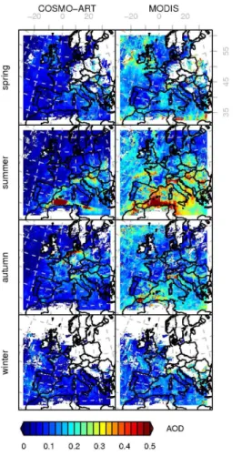
3.3.2 Aerosol optical depth

15

For comparison with MODIS AOD data, a similar procedure was employed as for OMI NO2vertical tropospheric columns, only using grid points for which satellite data were

available and which were cloud-free also in the model. The whole vertical column in the model was used in the calculation of aerosol optical depth with the method described in Vogel et al. (2009). All aerosol categories (internally and externally mixed Aitken and 20

accumulation modes, soot, mineral dust and sea salt modes) contribute to calculated AOD. Then, the median was calculated over the whole simulation period. We chose the median instead of the mean to be more robust against outliers. Figure 7 presents the results. Furthermore, as for the comparison with OMI NO₂ VTCs, aggregated biases have been calculated and can be found in Table 2.

25

(22)

GMDD

4, 1809–1874, 2011

C. Knote et al.

Title Page

Tables Figures

◭ ◮

Back Close

Full Screen / Esc

Discussion

P

a

per

|

Dis

cussion

P

a

per

|

Discussion

P

a

per

|

Discussio

n

P

a

per

|

log-log space. In case MODIS data was available also this information was added to the plots. The results for the summer 2006 period are shown in Fig. 8, plots for the remaining seasons can be found in the Supplement, and Table 2 shows the mean biases for these comparisons.

The comparison against these two independent sets of AOD measurements leaves 5

a mixed picture: compared with MODIS, the model shows consistently lower values than derived from the satellite. We can capture regions with continuously high AOD values like the Po valley (northern Italy) or Saharan dust events like e.g. in the summer 2006 period over the western Mediterranean Sea. The magnitude of the dust event is underestimated, which might be explained by the fact that modelled “dust” is only 10

created within the region of the model domain which covers only a small part of the Sa-hara. Contribution of sea salt to AOD is visible over the Atlantic ocean, but the absolute values are much lower than MODIS derived values, except for winter 2006. Some very polluted regions in south-eastern Europe are captured in location and magnitude (e.g. in Northern Croatia/Southern Hungary), while several other “hot-spots” visible from the 15

satellite (e.g. Eastern UK coast) are missed.

Comparison with AERONET station data reveals additional details. Although the ab-solute levels are often too low, which is consistent with our comparison with MODIS data, the temporal evolution is often well represented and most high AOD events visi-ble in station data are also observed in our simulations. Di_fferences between MODIS 20

and AERONET derived AOD on the other hand are at several occasions as big as the differences between model and AERONET, and non-negligible on average (up to 10 % compared to up to 60 % di_fference between model and measurements, see Table 2). We suggest that the role of water in the aerosol will play a major role in the differences found. Both, MODIS and AERONET data, are “cloud-screened”, i.e. data points con-25

(23)

GMDD

4, 1809–1874, 2011

C. Knote et al.

Title Page

Tables Figures

◭ ◮

Back Close

Full Screen / Esc

Discussion

P

a

per

|

Dis

cussion

P

a

per

|

Discussion

P

a

per

|

Discussio

n

P

a

per

|

2009) near regions with missing (cloud-screened) pixels. Also in several AERONET stations the sudden steep increase of AOD just before measurements are filtered (for clouds) can be found. While we tried to remove this error by using median values in-stead of the arithmetic mean to calculate the MODIS-model comparison, we probably could not exclude all of those situations. As the effect is non-linear and acts towards 5

very high AOD values, this will probably bias AOD results.

A clear negative bias in absolute AOD is seen in our model when compared with two independent measurement datasets which appears to be consistent with the too low simulated PM10 and PM2.5 levels. Fair correlation of the evolution in time is visible

from the AERONET comparison. Performance of our AOD simulations is well in range 10

of results for comparable modeling systems (e.g. Zhang et al., 2010; Aan de Brugh et al., 2011). We argue that both missing aerosol mass at the lateral boundaries and inaccuracies of simulated aerosols within the domain contribute to the underestimated AOD. Especially for aerosol components from natural sources (Saharan dust) the miss-ing lateral contribution could be substantial. Although we tried to remedy this by usmiss-ing 15

averaged profiles from a previous run, we could not – especially for those categories – represent the absolute mass contributions correctly. The impact of the missing pathway to form sulfate in clouds and the known too small yield of SOA in the SORGAM model are additional sources of error that impact the overall accuracy of the comparison.

3.3.3 Chemical composition

20

Aerosol chemical composition was evaluated by comparison with AMS data. In sum-mer 2006, AMS measurements were available at Payerne (CH), Harwell (UK) and Bush (UK) (Lanz et al., 2010). Several AMS instruments were deployed during the 2008 (autumn) and 2009 (spring) periods at stations throughout Europe. Timelines of the composition of NR−PM1are presented for both measurement and simulation at these

25

(24)

GMDD

4, 1809–1874, 2011

C. Knote et al.

Title Page

Tables Figures

◭ ◮

Back Close

Full Screen / Esc

Discussion

P

a

per

|

Dis

cussion

P

a

per

|

Discussion

P

a

per

|

Discussio

n

P

a

per

|

represent each species: ammonium (NH₄) in orange, sulfate (SO₄) in red, and nitrate (NO3) in blue. Organic aerosols (OA) are represented as shades of green. Charges

are omitted intentionally for the AMS in the figure legends, as also contributions from organosulfates, organonitrates are included which are not ions (Farmer et al., 2010). In case of modelled values, a distinction can be made between anthropogenic primary or-5

ganics (aPOA), secondary organics from anthropogenic (aSOA) and biogenic (bSOA) sources. Table2 presents the mean biases for each species over all stations in each season.

At all stations the time evolution of NR−PM1is represented well by our simulations.

Single events with higher aerosol concentrations (e.g. in Vavihill, 2008, Fig. 9) cor-10

respond in time and magnitude with the observations in most cases. Several model deficiencies can also be seen throughout the comparison, namely an overestimation of nitrate components and an underestimation of sulfate and, sometimes, organic mass. In the following we will briefly discuss the result for each station.

In Switzerland, measurements at Payerne were available for three periods. The 15

time evolution of total aerosol mass corresponds best in spring 2009, and worst in the summer 2006 period. The weak correlation in summer 2006 is mostly due to a se-vere underestimation of OA, especially during daytime hours, and an ose-verestimation of nitrate during nighttime. In spring 2009, several abrupt changes in aerosol mass concentrations were observed. Although the timing is not the same each time, the 20

model reproduces those changes. A tendency to retain too much nitrate in the aerosol phase during daytime is apparent. Sulfate is underestimated. During autumn 2008, an episode of high aerosol concentrations is observed in the middle of the observation period. This is also reported by the model. OA are, however, underestimated, and ni-trate aerosols overestimated. Here also, modelled aerosol nini-trate shows a persistence 25

(25)

GMDD

4, 1809–1874, 2011

C. Knote et al.

Title Page

Tables Figures

◭ ◮

Back Close

Full Screen / Esc

Discussion

P

a

per

|

Dis

cussion

P

a

per

|

Discussion

P

a

per

|

Discussio

n

P

a

per

|

sulfate is in the same range as in Payerne, and therefore even more strongly underes-timated. The concentrations of organics are lower in Melpitz, and simulated values are comparable here. The third station with more than one period of measurements is Vav-ihill (SE). Generally low aerosol concentrations alternate with bursts in aerosol mass with high contents of inorganic secondary components. This burst pattern is captured 5

in our simulations, and also the timing fits mostly well. Especially in spring 2009 the model lacks, though, the OA mass necessary to fit the measurements. While ammonia levels are comparable in autumn 2008, they are above measured levels in spring 2009. The AMS deployed at Hyyti ¨al ¨a reports very low NR−PM1 concentrations, with large

contributions by sulfate and OA, and, in spring 2009, almost no nitrate. The model can 10

represent the overall level of aerosol concentration. However, the simulations signifi-cantly underestimate sulfate and overestimate nitrate.

All other stations only report data for one period. In autumn 2008, measurements of aerosol chemical composition were also available for K-Puszta, Hungary. The station reported high aerosol concentrations with levels up to 30 µg m−3_{total mass. While the}

15

model represents the build-up of aerosols towards the middle of the observation pe-riod, the overall mass is underestimated. Too high nitrate levels are simulated. Organ-ics and ammonium match observations better, but sulfate tends to be understimated also at this location. Four more stations reported data during spring 2009: Cabauw (NL), Helsinki (FI), Barcelona (ES) and Montseny (ES). Cabauw (NL) has lower con-20

centrations than e.g. Payerne or Melpitz, and a big gap in measurements during the first half of our simulations. There is some resemblence in the peaks of aerosol mass during the second half of the simulation between model and station values. Nitrates are overestimated while ammonium and sulfate are too low. Organics are well cap-tured. Helsinki (FI), an urban background station is, like Hyyti ¨al ¨a (FI) characterized by 25

(26)

GMDD

4, 1809–1874, 2011

C. Knote et al.

Title Page

Tables Figures

◭ ◮

Back Close

Full Screen / Esc

Discussion

P

a

per

|

Dis

cussion

P

a

per

|

Discussion

P

a

per

|

Discussio

n

P

a

per

|

et al., 1993) which are still found to be underestimated in current emission inventories (Prank et al., 2010). Additionally, due to the setup of aerosol boundary conditions in our modeling system, we very likely underestimate direct sulfate inflow in this region. In Barcelona (ES), also an urban background location, a very variable time series is reported, with the highest absolute concentrations of all stations used in this analysis. 5

Several peaks of aerosol concentration each day are common, containing relatively high sulfate levels compared to other stations. The model produces a similar variability, although it overestimates nitrate. Sulfate levels are comparable at this site with a large influence from shipping. OA concentrations are, in contrast to most other stations, over-estimated at Barcelona and Helsinki. The largest contributor to simulated total organic 10

mass at these stations is primary emitted organics. Statistical analysis of the organic fraction (positive matrix factorization (PMF), Paatero and Tapper, 1994) indicates that organics in urban stations are comprised of similar amounts of SOA and POA, while in the model it is almost exclusively POA. This points towards a strong underestimation of secondary organics in polluted regions as it has been found already by Fast et al. 15

(2009). Finally, the AMS in Montseny (ES) measured a time-series with several peri-ods with increased aerosol loadings, and during the first third a period where almost no aerosols were found due to an episode of strong Atlantic advection. The model cap-tures this period well. Total organics are comparable throughout the simulation period, although a PMF analysis gives about 5 % mass contribution from urban primary organ-20

ics (M.C. Minguillon, 2011), instead of about 30 % as given in the model. Nitrates are too high, and lacking the diurnal cycle visible in the measurement. Simulated sulfate is below measurements.

3.3.4 Number concentrations and size distributions

The dataset compiled by Asmi et al. (2011) provides a homogenized overview of the 25

(27)

GMDD

4, 1809–1874, 2011

C. Knote et al.

Title Page

Tables Figures

◭ ◮

Back Close

Full Screen / Esc

Discussion

P

a

per

|

Dis

cussion

P

a

per

|

Discussion

P

a

per

|

Discussio

n

P

a

per

|

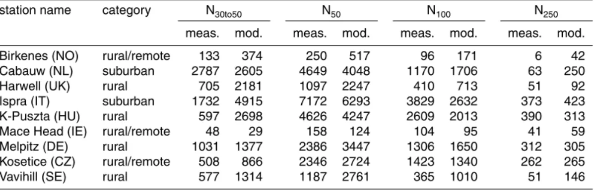
and 100 (N₁₀₀) nm up to 500 nm have been chosen as proxies to study climate effects. Health concerns are related to very small particles, which are assessed by comparing number concentrations of particles between 30 and 50 nm (N_30to50). This concentration can also serve as an indicator of new particle formation and emissions from combustion processes. Finally, the number of particles with diameters between 250 and 500 nm 5

(N₂₅₀) are given to show the contribution of larger particles to total aerosol number concentrations. We have calculated the corresponding model values by integrating the aerosol modes over the respective intervals. Data were available in up to hourly resolution, so a direct comparison could be made between modelled and simulated values. Table 3 shows the resulting comparison for the autumn 2008 period, the table 10

for 2009 can be found in the Supplement. Table 2 gives a summary overview of the mean biases over all stations.

We also studied the histograms (occurence distribution) of logarithms of the num-ber concentrations in the particle size ranges (not shown). The analysis was done in logarithmic concentration space as most of the aerosol number concentrations are 15

log-normally distributed (Asmi et al., 2011). It shows the model’s ability to produce sim-ilar distributions of number concentrations as measured and provides a more detailed way to analyze the differences. We also performed a Mann-Whitney U-test (Higgins, 2004) on the modelled and measured concentration distributions to see with what p-value they could be considered to be from the same distribution with similar mean and 20

distribution shape.

The histograms of number concentrations show relatively good agreement between modelled and measured concentrations. Overall the agreement is better in greater diameter size ranges (N₁₀₀ and N₂₅₀) in comparison to concentrations in N_30to50size range. The model seems to overestimate the number concentrations in the smaller 25

(28)

GMDD

4, 1809–1874, 2011

C. Knote et al.

Title Page

Tables Figures

◭ ◮

Back Close

Full Screen / Esc

Discussion

P

a

per

|

Dis

cussion

P

a

per

|

Discussion

P

a

per

|

Discussio

n

P

a

per

|

does not generally produce the observed amounts of nucleated particles in the Eu-ropean boundary layer. Thus the overestimation could be due to a disproportioned amount of emitted sulphur to be considered as primary Aitken particles, which have a much higher lifetime in the atmosphere compared to newly nucleated particles in these regions. For the larger particle sizes (N₁₀₀ and N₂₅₀), the model-measurement 5

comparison is more successful. At Central European stations the modelled and mea-sured concentration distributions are generally of similar shape and median, which is well demonstrated by p-values ranging from 0.31 to 0.66 in the U-test test parameter for Kosetice and Melpitz. The overall shapes of the concentration histograms are gen-erally similar in all the stations, although some discrepancies in lower-concentration 10

regions are visible. The agreement is generally poorer in lower-concentration regions of Northern Europe, but also in Cabauw (NL) and Harwell (UK)N₂₅₀ concentrations, where the model overestimated the concentrations by a factor of 2 in 2008.

A second dataset available from Asmi et al. (2011) is seasonal statistics of aerosol number size distributions. We have calculated a distribution function as mean over 15

all modelled values in each simulation period, and compared it against the measured distribution statistics of the corresponding season (Fig. 11 for autumn 2008, plots for spring 2009 can be found in the Supplement. Note that there is no exact match be-tween the time periods covered by the measurements and the simulations (3 weeks out of the 3 months). Overall, the modelled size distributions are close to the observed 20

ones. At most stations, simulated size distributions were within the central 67 % per-centiles of the values reported by Asmi et al. (2011) when comparing the 20 to 200 nm size range, for which the instruments were reported to compare the best (Wieden-sohler et al., 2010). Concerning the shape of the size distributions, stations with the best match between model and measurements were Melpitz (DE), Waldhof (DE) and 25