REAL-TIME VISUAL SLAM USING PRE-EXISTING FLOOR LINES AS LANDMARKS AND A SINGLE CAMERA
Andre S. MACEDO∗, Gutemberg S. SANTIAGO∗, Adelardo A.D. MEDEIROS∗
∗Departement of Computer Engineering and Automation (DCA) Federal University of Rio Grande do Norte (UFRN), Natal RN Brazil
Emails: [andremacedo, gutemberg, adelardo]@dca.ufrn.br
Abstract— This work proposes a SLAM (Simultaneous Localization and Mapping) technique based on Ex-tended Kalman Filter (EKF) to navigate a robot in an indoor environment using odometry and pre-existing lines on the floor as landmarks. The lines are identified by using the Hough transform. The prediction phase of the EKF is implemented using the odometry model of the robot. The update phase directly uses the parameters of the lines detected by the Hough transform without additional intermediate calculations. Experiments with real data are presented.
Keywords— SLAM; Kalman filter; Hough transform
Resumo— Este trabalho prop˜oe uma t´ecnica para SLAM (Simultaneous Localization and Mapping) baseada no filtro de Kalman estendido (EKF) para navegar um robˆo em um ambienteindoorusando odometria e linhas pr´e-existentes no ch˜ao como marcos. As linhas s˜ao identificadas usando a transformada de Hough. A fase de predi¸c˜ao do EKF ´e feita usando o modelo de odometria do robˆo. A fase de atualiza¸c˜ao usa diretamente os parˆametros das linhas detectados pela transformada de Hough sem c´alculos adicionais intermedi´arios. S˜ao apresentados experimentos com dados reais.
Palavras-chave— SLAM; Filtro de Kalman; Transformada de Hough
1 Introduction
In the problem of simultaneous localization and mapping (SLAM), a mobile robot explores the en-vironment with its sensors, gains knowledge about it, interprets the scene, builds an appropriate map and localizes itself relative to this map. The rep-resentation of the maps can take various forms, such as occupancy grids and features maps. We are interested in the second representation.
Thanks to advances in computer vision and cheaper cameras, vision-based SLAM have be-come popular (Goncalves et al., 2005; Mouragnon et al., 2006; Jensfelt et al., 2006). In the work of Folkesson et al. (2005), lines and points were extracted by image processing and used to solve the SLAM problem. Chen and Jagath (2006) pro-posed a SLAM method with two phases. Firstly, high level geometric information, such as lines and triangles constructed by observed feature points, is incorporated to EKF to enhance the robustness; secondly, a visual measurement approach, based on multiple view geometry, is employed to initial-ize new feature points.
A classical approach to SLAM is to use Ex-tended Kalman Filter (EKF) (Dissanayake et al., 2001; Castellanos et al., 2001). These SLAM al-gorithms usually require a sensor model that de-scribes the robot’s expected observation given its position. Davison (2003) uses a single camera, assuming a Gaussian noise sensor model whose covariance is determined by the image resolu-tion. Zucchelli and Koˇseck´a (2001) discusse how to propagate the uncertainty of the camera’s in-trinsic parameters into a covariance matrix that
characterizes the noisy feature positions in the 3D space. Wu and Zhang (2007) present a work whose principal focus is on how to model the sensor un-certainty and build a probabilistic camera model. The main challenges in visual SLAM are: a) how to detect features in images; b) how to recog-nize that a detected feature is or is not the same as a previously detected one; c) how to decide if a new detected feature will or will not be adopted as a new mark; d) how to calculate the 3D po-sition of the marks from 2D images; and e) how to estimate the uncertainty associated with the calculated values. In the general case, all these aspects have to be addressed. However, in partic-ular situations, it is sometimes possible to develop a specific strategie to overcome these difficulties. That is the proposal of this work.
2 Theoretical background 2.1 Extended Kalman filter
In this work, the Extended Kalman Filter (EKF) deals with a system modeled by System 1, whose variables are described in Table 1. εt and δt are
supposed to be zero-mean Gaussian white noises.
(
st=p(st−1,ut−1, εt−1)
zt=h(st) +δt
(1)
At each sampling time, the EKF calculates the best estimate of the state vector in two phases:
• theprediction phaseuses System 2 to pre-dict the current state based on the previous state and on the applied input signals; • theupdate phaseuses System 3 to correct
the predicted state by verifying its compati-bility with the actual sensor measurements.
( ¯
µt=p(µt−1,ut−1,0) ¯
Σt=GtΣt−1GTt +VtMtVTt
(2)
Kt= ¯ΣtHTt(HtΣ¯tHTt +Qt)−1 µt= ¯µt+Kt(zt−h(¯µt))
Σt= (I−KtHt) ¯Σt
(3)
where:
Gt=
∂p(s,u, ε) ∂s
s=µt−1,u=ut−1,ε=0
(4)
Vt= ∂p(s,u, ε) ∂ε
s=µt
−1,u=ut−1,ε=0
(5)
Ht= ∂h(s) ∂s
s=µt
−1
(6)
Table 1: Symbols in Equations (1), (2) and (3)
st state vector (order n) at instantt p(·) non-linear model of the system
ut−1 input signals (orderl), instantt−1 εt−1 process noise (order q), instantt−1
zt vector of measurements (order m) re-tourned by the sensors
h(·) non-linear model of the sensors δt measurement noise
¯
µt,µt mean (order n) of the state vector st,
before and after the update phase ¯
Σt,Σt covariance (n×n) of the state vectorst Gt Jacobian matrix (n×n) that linearizes
the system modelp(·)
Vt Jacobian matrix (n×q) that linearizes
the process noise εt
Mt covariance (q×q) of the process noiseεt Kt gain of the Kalman filter (n×m)
Ht Jacobian matrix (m×n) that linearizes the model of the sensorsh(·)
Qt covariance matrix (m×m) of the mea-surement noiseδt
∆L
y ∆θ
x b
r ∆θL
∆θR
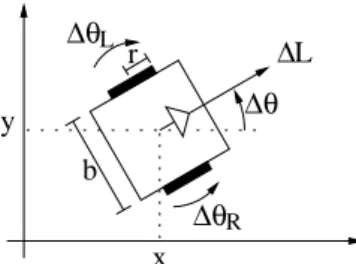
Figure 1: Variables of the kinematic model
2.2 EKF-SLAM
In SLAM, besides estimating the robot pose, we also estimate the coordinates of all landmarks en-countered along the way. This makes necessary to include the landmark coordinates into the state vector. Ific is the vector of coordinates of the
i-th landmark and i-there arek landmarks, then the state vector is:
st= xtytθt
1 cT
t · · · kcT
t
T
(7)
When the number of marks (k) is a priori
known, the dimension of the state vector is static; otherwise, it grows up when a new mark is found.
3 Modeling 3.1 Prediction phase: process model
Consider a robot with diferential drive in which ∆θR and ∆θL are the right and left angular
dis-placement of the respective wheels, according to Figure 1. Assuming that the speeds can be con-sidered constant during one sampling period, we can determine the kinematic geometric model of the robot’s movement (System 8):
xt=xt−1+ ∆L
∆θ[sin(θt−1+∆θ)−sin(θt−1)]
yt=yt−1− ∆L
∆θ[cos(θt−1+∆θ)−cos(θt−1)] θt=θt−1+ ∆θ
(8)
in which:
(
∆L= (∆θRrR+ ∆θLrL)/2
∆θ= (∆θRrR−∆θLrL)/b
(9)
where ∆Land ∆θare the linear and angular dis-placement of the robot;b represents the distance between wheels and rR and rL are the radii of
the right and the left wheels, respectively. When ∆θ → 0, the model becomes the one in Equa-tion 10, obtained from the limit of System 8.
xt=xt−1+ ∆Lcos(θt−1) yt=yt−1+ ∆Lsin(θt−1) θt=θt−1
(10)
as input signals to be incorporated to the robot’s model, rather than as sensorial measurements. The differences between the actual angular dis-placements of the wheels (∆θR and ∆θL) and
those ones measured by the encoders (∆˜θR and
∆˜θL) are modeled by a zero mean Gaussian white
noise, accordingly to System 11.
(
∆θR= ∆˜θR+εR
∆θL= ∆˜θL+εL
(11)
The measured ∆ ˜Land ∆˜θare defined by replacing (∆θRand ∆θL) by (∆˜θRand ∆˜θL) in Equations 9.
If the state vector s is given by Equation 7, the system model p(·) can be obtained from Sys-tems 8 or 10 and from the fact that the landmarks coordinatesic are static:
p(·) =
xt=· · ·
yt=· · ·
θt=· · ·
1 ct=
1 ct−1 .. .
kc
t=kct−1
n= 3 +k·order(ic) (12)
ut=
h
∆˜θR∆˜θL
iT
l= 2 (13)
εt= [εRεL]T q= 2 (14)
TheGandVmatrices are obtained by deriv-ing thep(·) model1
using Equations 4 and 5:
G=
1 0 g13 0 · · · 0 0 1 g23 0 · · · 0 0 0 1 0 · · · 0 0 0 0 1 · · · 0
..
. ... ... ... ... 0 0 0 0 · · · 1
(15)
where:
g13= ∆ ˜L
∆˜θ[cos(θt−1+ ∆˜θ)−cos(θt−1)]
g23= ∆ ˜L
∆˜θ[sin(θt−1+ ∆˜θ)−sin(θt−1)]
V=
v11 v12 v21 v22 rR/b −rL/b
0 0
.. . ...
0 0
(16)
1
We only present theGandVmatrices using thep(·)
model based on Equations 8. Other matrices can be ob-tained by deriving Equations 10 to be used when ∆θ→0.
Figure 2: Robotic system.
where, consideringrR=rL=r:
v11=V1cos(β) +V2[sin(β)−sin(θt−1)] v12=−V1cos(β) +V3[sin(β)−sin(θt−1)] v21=V1sin(β)−V2[cos(β)−cos(θt−1)] v22=−V1sin(β)−V3[cos(β)−cos(θt−1)]
β =θt−1+
r(∆˜θR−∆˜θL)
b V1=
r(∆˜θR+ ∆˜θL)
2(∆˜θR−∆˜θL)
V2=
−b∆˜θL
(∆˜θR−∆˜θL)2
V3=
b∆˜θR
(∆˜θR−∆˜θL)2
It is well known that odometry introduces ac-cumulative error. Therefore, the standard devi-ation of the noises εR and εL is assumed to be
proportional to the module of the measured an-gular displacement. These considerations lead to a definition of the matrixMgiven by Equation 17.
M=
(MR|∆˜θR|)
2
0 0 (ML|∆˜θL|)2
(17)
3.2 Update phase: sensor model
The landmarks adopted in this work are lines formed by the grooves of the floor in the envi-ronment where the robot navigates. The system is based on a robot with differential drive and a fixed camera, as in Figure 2.
The landmarks are detected by processing im-ages using the Hough transform (see Section 4). The detected lines are described by the parame-tersρand αin Equation 18:
ρ=xcos(α) +ysin(α) (18)
Figure 3 shows the geometric representation of these parameters: ρ is the module and α is the angle of the shortest vector connecting the origin of the system of coordinates to the line.
Y
α ρ
X
XF YF
F
xM
F M θ
YM X
M
F
yM
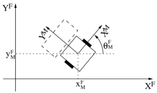
Figure 4: Mobile and fixed coordinate systems
We define a fixed coordinate system (F) and a mobile one (M), attached to the robot, both illustrated in Figure 4. The origin of the mo-bile system has coordinates (xF
M, y F
M) in the fixed
system. θF
M represents the rotation of the
mo-bile system with respect to the fixed one. One should note that there is a straight relation among these variables (xM
F, y M F , θ
M
F ) and the robot’s pose
(xt, yt, θt), which is given by Equations 19.
xt=xMF yt=yFM θt=θMF +π/2 (19)
Each line on the floor is described by two static parameters (ρF, αF). The map to be
pro-duced by the SLAM process is composed of a set of these pairs of parameters. So, the ic vector of
coordinates of the i-th landmark that appears in Equations 7 and 12 is given by Equation 20:
ic=
iρF
iαF
(20)
At each step the robot captures an image and identifies the parameters (˜ρ,α)˜ 2
of the detected lines. These image parameters are then con-verted to the corresponding parameters (˜ρM, α˜M)
in the mobile coordinate system M attached to the robot, using the camera parameters (see Sec-tion 4). The vector of measurementsztto be used
in the update phase of the EKF algorithm (Equa-tion 3) is defined by Equa(Equa-tion 213
:
zt=
˜ ρM
˜ αM
(21)
To use information directly obtained by image processing (˜ρM,α˜M) in the update phase of the
EKF-SLAM, one must deduct the sensor model h(·), that is, the expected value of these parame-ters in function of the state variables
We use the relation between coordinates in theM andFsystems (Sistem 22) and Equation 18 in both coordinate systems (Equations 23 and 24):
2
We use a˜over a variable to indicate measured values, rather than calculated ones.
3
To simplify the notation, we are assuming that there is exactly one line per image. In fact, we can have none, one or more than one line per image. At each step, we execute the update phase of the EKF as many times as the number of detected lines in the image, even none.
(
xF = cos(θM F )x
M−sin(θM F)y
M +xF M
yF = sin(θM
F )xM + cos(θMF)yM +yFM
(22)
iρF =xFcos(iαF) +yFsin(iαF) (23)
ρM =xMcos(αM) +yMsin(αM) (24)
By replacing Equations 22 in Equation 23, doing the necessary equivalences with System 24 and re-placing some variables using Equations 19, we ob-tain the Systems 25 and 26, which represent two possible sensor modelsh(·) to be used in the filter. To decide about which model to use, we calculate both values ofαM and use the model which
gen-erate the value closer to the measured value ˜αM.
(
ρM =iρF−x
tcos(iαF)−ytsin(iαF)
αM =iαF−θ t+π/2
(25)
(
ρM =−iρF+x
tcos(iαF) +ytsin(iαF)
αM =iαF−θ t−π/2
(26)
The sensor model is incorporated into the EKF through theH matrix (Equation 6), given by Equation 274
:
H=
−cosiαF −siniαF 0 · · · 1 0 · · ·
0 0 −1 · · · 0 1 · · ·
(27)
The final columns of theH matrix are almost all null, except for the columns corresponding to the landmark in the vector state that matchs the de-tected line on the image.
3.3 Matching
A crucial aspect of the SLAM algorithm is to es-tablish a match between the detected line on the image and one of the landmarks represented in the state vector. To choose the correct landmark, we first calculate the predicted values of (ρF, αF)
using the measured values of (˜ρM,α˜M) and the
model in Equations 25, if ˜αM ≥ 0, or in
Equa-tions 26, if ˜αM <0. Then, these predicted values
are compared to each one of the values (iρF,iαF)
in the state vector. If the difference between the predicted values and the best (iρF, iαF) is small
enough, a match was found. If not, we consider that a new mark was detected and the size of the state vector is increased.
4 Image processing 4.1 Detection of lines
Due to the choice of floor lines as landmarks, the technique adopted to identify them was the Hough transform (Gonzalez and Woodes, 2000). The
4
Figure 5: Detection of lines
purpose of this technique is to find imperfect in-stances of objects within a certain class of shapes by a voting procedure. This voting procedure is carried out in a parameter space, from which ob-ject candidates are obtained as local maxima in a accumulator grid that is constructed by the algo-rithm for computing the Hough transform.
In our case, the shapes are lines described by Equation 18 and the parameter space has coordi-nates (ρ, α). The images are captured in grayscale and converted to black and white using a thresh-old level, determined off-line. Figure 5 shows a typical image of the floor and the lines detected by the Hough transform.
4.2 From images to the world
We assume that the floor is flat and that the cam-era is fixed. So, there is a constant relation (a homographyA) between points in the floor plane (x, y) and points in the image plane (u, v):
s·
u v 1
=A·
x y 1
(28)
The scale factorsis determined for each point in such a way that the value of the third element of the vector is always 1.
The homography can be calculated off-line by using a pattern containing 4 or more remarkable points with known coordinates (see Figure 6). Af-ter detecting the remarkable point in the image,
Figure 6: Calibration pattern
XF YF
1.08 2.16 3.24
0.98 1.96 2.94
Figure 7: Executed trajectory
we have several correspondences between point co-ordinates in the mobile coordinate systemM and in the image. Replacing these points in Equa-tion 28, we obtain a linear system with which we can determine the 8 elements5
of the homograpy matrixA.
Once calculated the homography, for each de-tected line we do the following:
1. using the values of (˜ρ,α) in the image ob-˜ tained by the Hough transform, calculate two point belonging to the image line;
2. convert the coordinates of these two points to the mobile coordinate systemaM;
3. determine (˜ρM,α˜M) of the line that passes
through these two points.
5 Results
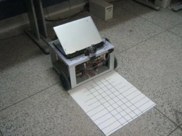
The experiments were conducted using the robot Karel6
, a mobile reconfigurable platform con-structed in our laboratoy (see Figure 6). It has two wheels driven by DC motors with diferential drive. Each motor has an optical encoder and a dedi-cated board based on a PIC microcontroller that carries out a local velocity control. The boards communicate with a computer through a CAN bus, receiving the desired velocities of the wheels and sending data from the encoders.
The computer that controls the robot is an ordinary notebook with an USB-CAN bridge and a color webcam connected to its USB bus. The camera captures 160×120 images (as the one in Figure 5) and each image is processed in 300ms.
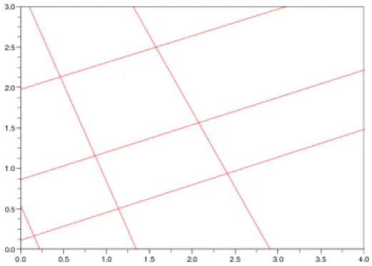
We present here an experiment in which the robot executes a forward mouvement, turnes over itself and retournes close to the original posi-tion. In Figure 7 we indicate the position of the lines, the approximated trajectory of the robot and the comparative size of the camera’s field of view. The initial position of the robot is roughly (3.3,3.1,110o), but it is not used in the SLAM
algorithm: the robot assumes that its initial posi-tion is (0,0,0o)
5
Acan only be determined up to a scale factor. To obtain a unique answer, we imposea33= 1.
6
Table 2: Experimental results Actual Calculated Corrected
ρ α ρ α ρ α
1.08 0 1.88 108 1.13 1.7 2.16 0 0.82 108 2.19 1.3 3.24 0 0.11 110 3.26 0 0.98 90 2.57 23 0.97 87 1.96 90 1.24 22 1.95 87 2.94 90 0.20 22 2.93 88
Table 2 presents the detected landmarks af-ter approximately 250 iaf-teractions. The first two columns contain the actual values. The result of the SLAM algorithm is in the second two columns: the values are expressed in the coordinate sys-tem assuming that the initial robot position is (0,0,0o). These lines are drawn in Figure 8.
Fi-nally, the last two columns show the SLAM result but corrected by assuming the initial robot posi-tion as (3.3,3.1,110o), for better comparison.
6 Conclusions and Perspectives
The main contribution in this paper is the model-ing of the optical sensor made in such a way that it permits using the parameters obtained by the image processing algorithm directly into the equa-tions of the EKF, without intermediate phases of pose or distance calculation. The values pre-sented in Table 2 demonstrate that the proposed approach can obtain good results even with a rel-atively small quantity of samples.
As future works, we intend to improve the retime properties of the image processing al-gorithm, by adopting some of the less time-consuming variants of the Hough transform. An-other required improvement is to deal with line segments with finite length, incorparating this characteristics to the step of matching lines.
Thanks
Andr´e Macedo was financially supported by CNPq during this work.
Figure 8: Lines calculated by EKF-SLAM
References
Castellanos, J., Neira, J. and Tardos, J. (2001). Multisensor fusion for simultaneous localiza-tion and map building, IEEE Transactions on Robotics and Automation 17(6).
Chen, Z. and Jagath, S. (2006). A visual SLAM solution based on high level geometry knowl-edge and Kalman filtering, IEEE Canadian Conference on Electrical and Computer En-gineering.
Davison, A. J. (2003). Real-time simultaneous lo-calisation and mapping with a single camera,
IEEE International Conference on Computer Vision, Vol. 2, Nice, France, pp. 1403–1410.
Dissanayake, M. G., Newman, P., Clark, S. and Durrant-Whyte, H. F. (2001). A solution to the simultaneous localization and map build-ing (SLAM) problem,IEEE Transactions on Robotics and Automation17(3).
Folkesson, J., Jensfelt, P. and Christensen, H. I. (2005). Vision SLAM in the measurement subspace,IEEE International Conference on Robotics and Automation, pp. 30–35.
Goncalves, L., di Bernardo, E., Benson, D., Sved-man, M., Ostrovski, J., Karlsson, N. and Pirjanian, P. (2005). A visual front-end for simultaneous localization and mapping,
IEEE International Conference on Robotics and Automation, pp. 44–49.
Gonzalez, R. C. and Woodes, R. E. (2000).
Processamento de Imagens Digitais, Edgard Blucher. ISBN: 8521202644.
Jensfelt, P., Kragic, D., Folkesson, J. and Bj¨ork-man, M. (2006). A framework for vision based bearing only 3D SLAM,IEEE Interna-tional Conference on Robotics and Automa-tion, pp. 1944– 1950.
Mouragnon, E., Lhuillier, M., Dhome, M., Dekeyser, F. and Sayd, P. (2006). 3D re-construction of complex structures with bun-dle adjustment: an incremental approach,
IEEE International Conference on Robotics and Automation, pp. 3055–3061.
Thrun, S., Burgard, W. and Fox, D. (2005). Prob-abilistic Robotics, 1 edn, MIT Press, USA. ISBN 978-0262201629.
Wu, J. and Zhang, H. (2007). Camera sen-sor model for visual SLAM,IEEE Canadian Conference on Computer and Robot Vision.