Pushpa N. Rathie
Department of Statistics and Applied Mathematics Federal University of Ceara
Fortaleza, CE, Brazil. [email protected]
Paulo H. D. Silva Department of Statistics
University of Brasilia Brasilia, Brazil.
Abstract
This paper deals with three new generalized ceiling density functions, their distribution functions and moments. Graphical representations of the density and distribution functions are also given for various values of the parameters. The distributions functions, for the two corresponding generalized floor density functions given earlier, are also derived and represented graphically for various values of the parameters. Expression for moments are also given.
Mathematics Subject Classification: 60E05, 62B15, 33C60, 60E10.
Keywords: Generalized ceiling distribution, generalized floor distribution, mo-ments.
1
Introduction
In this paper, three new generalized ceiling distributions are introduced and their distribution functions and moments are derived. The density and distribution func-tions are graphically shown for various values of the parameters.
The distribution functions and moments for the corresponding two generalized floor distributions given earlier in [1] are also derived. The distribution functions are graphically represented for various values of the parameters.
2
Generalized Ceiling Distributions
2.1
Generalized Ceiling Distribution - I
The generalized ceiling distribution g1(x) of a random variable X, for x ≥ 1, is
defined by
g1(x) =d1(a, b)x−aeb⌈lnx⌉, (1)
withx≥1, a >1 +b, where
d1(a, b) =
(a−1) 1−e−(a−1−b)
eb 1−e−(a−1) . (2)
The constantd1(a, b) is determined from
1 = d1(a, b)
Z ∞
1
x−aeb⌈lnx⌉dx
= d1(a, b)
Z ∞
0
e−(a−1)y+b⌈y⌉dy,
by substitutinglnx=y. Thus,
1 = d1(a, b)
∞
X
n=0 eb(n+1)
Z n+1
n
e−(a−1)ydy
= d1(a, b) 1−a
∞
X
n=0
eb(n+1)he−(a−1)(n+1)−e−(a−1)ni
= d1(a, b)e
b e−(a−1)−1
(1−a) 1−e−(a−1−b). (3)
Hence (3) implies (2). The r-th moments about the origin is given by
E(Xr) = d1(a, b)
d1(a−r, b)
, r < a−1−b. (4)
The expression for mean, variance, kurtosis and skewness may be obtained from (4). The distribution functionG1(x) is given by
G1(x) = d1(a, b)
Z x
1
x−aeb⌈lnx⌉dx
= d1(a, b)
Z lnx
0
e−(a−1)y+b⌈y⌉dy
= d1(a, b)
⌈lnx⌉−2
X
n=0
eb(n+1)
Z n+1
n
e−(a−1)ydy+eb⌈lnx⌉
Z lnx
⌈lnx⌉−1
e−(a−1)ydy
,
G1(x) =
d1(a, b)
1−a
eb e−(a−1)−1
1−e−(a−1−b)(⌈lnx⌉−1)
1−e−(a−1−b)
!
+ d1(a, b)e b⌈lnx⌉
1−a
e−(a−1)lnx−e−(a−1)(⌈lnx⌉−1)
(5)
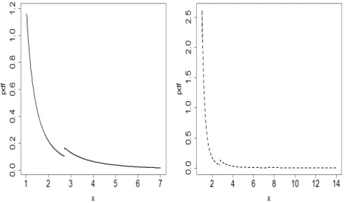
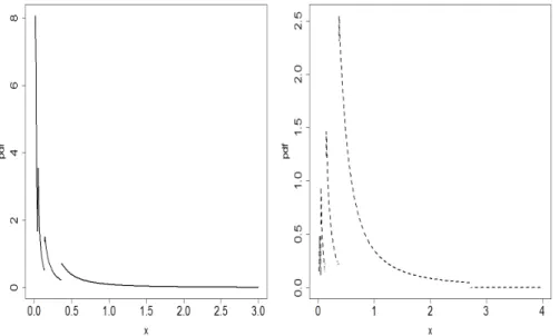
for x ≥ 1, a > 1 +b, where d1(a, b) is given by (2). The density g1(x) and the
distribution functionG1(x), for some values of the parameters aand b, are plotted
in Figure 1.
2.2
Generalized Ceiling Distribution - II
We define the generalized ceiling distribution g2(x) of a random variable X, for x >0, as
g2(x) =d2(a, b)x−ae−b⌈|lnx|⌉, x >0. (6)
The constantd2(a, b) is obtained from
1
d2(a, b)
=
Z ∞
0
x−aeb⌈|lnx|⌉dx
=
Z ∞
−∞
e−(a−1)y+b⌈|y|⌉dy
=
Z ∞
0
e−(a−1)y−b⌈y⌉dy+
Z ∞
0
e(a−1)y−b⌈y⌉dy
= 1
d1(a,−b)
+ 1
d1(2−a,−b) ,
whered1(a, b) is given in (2). Thus,
d2(a, b) =
d1(a,−b)d1(2−a,−b) d1(a,−b) +d1(2−a,−b)
, (7)
for 1−b < a <1 +b. The r-th moments about the origin is given by
E(Xr) = d2(a, b)
d2(a−r, b)
, (8)
fora−1−b < r < a−1 +b.
The corresponding distribution function G2(x) is obtained from
G2(x) = d2(a, b)
Z x
0
x−ae−b⌈|lnx|⌉dx
= d2(a, b)
Z lnx
−∞
e−(a−1)ye−b⌈|y|⌉dy.
(a) Left: a= 2.5 andb= 0.5. Right: a= 4 andb= 1
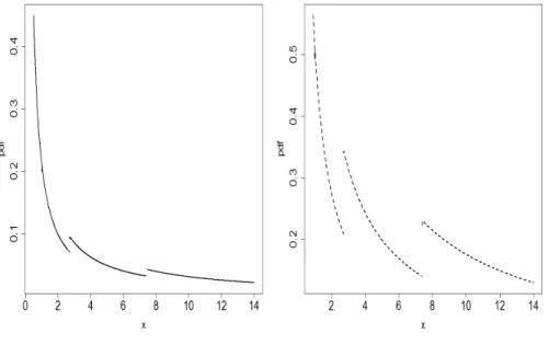
(b) Left: a= 2.5 andb= 0.5. Right: a= 4 and b= 1
• Subcase 1: x >1;
• Subcase 2: 0 < x <1.
Subcase 1: x >1
Forx >1,G2(x) is given by
G2(x) = d2(a, b)
Z 0
−∞
e−(a−1)ye−b⌈|y|⌉dy+
Z lnx
0
e−(a−1)ye−b⌈y⌉dy
= d2(a, b)
Z ∞
0
e(a−1)ye−b⌈y⌉dy+
Z lnx
0
e−(a−1)ye−b⌈y⌉dy
= d2(a, b)[I1+I2], (9)
suppose. Now,
I1 =
∞
X
n=0
e−b(n+1)
Z n+1
n
e(a−1)ydy
= e
−b ea−1−1
(a−1) 1−e−(b−a+1), b > a−1, (10)
as done in earlier subsection, and
I2 =
⌈lnx⌉−2
X
n=0
e−b(n+1)
Z n+1
n
e(a−1)ydy+e−b⌈lnx⌉
Z lnx
⌈lnx⌉−1
e−(a−1)ydy
= e
−b e−(a−1)−1
1−e−(a−1+b)(⌈lnx⌉−1)
(1−a) 1−e−(a−1+b)
+ e
−b⌈lnx⌉
1−a
h
x1−a−e−(a−1)(⌈lnx⌉−1)
i
, (11)
as done in earlier subsection. Subcase 2: 0< x <1
In this subcase,
G2(x) =d2(a, b)
Z ∞
−lnx
suppose. Here,
I3 =
Z ∞
⌈−lnx⌉
e(a−1)ye−b⌈y⌉dy+
Z ⌈−lnx⌉
−lnx
e(a−1)ye−b⌈y⌉dy
=
∞
X
n=⌈−lnx⌉
e−b(n+1)
Z n+1
n
e(a−1)ydy+e−b⌈−lnx⌉
Z ⌈−lnx⌉
−lnx
e(a−1)ydy
=
∞
X
n=⌈−lnx⌉
e−b(n+1)
"
e(a−1)(n+1)−e(a−1)n a−1
#
+e−b⌈−lnx⌉
"
e(a−1)⌈−lnx⌉−e(a−1)(−lnx) a−1
#
= 1
a−1
e−b ea−1−1
∞
X
n=⌈−lnx⌉
e−(b−a+1)n+e−b⌈−lnx⌉e(a−1)⌈−lnx⌉−e(a−1)(−lnx)
= e
−b ea−1−1
a−1
1
1−e−(b−a+1) −
1−e−(b−a+1)⌈−lnx⌉
1−e−(b−a+1)
!
+ e
−b⌈−lnx⌉
a−1
e(a−1)⌈−lnx⌉−e(a−1)(−lnx), (12)
forb > a−1. For some values of the parametersaandb,g2(x) andG2(x) are shown
in Figure 2.
2.3
Generalized Ceiling Distribution - III
The generalized ceiling density function g3(x) of a random variable X, for −∞ < x <∞, is given by
g3(x) =d3(a, b)|x|−ae−b⌈|ln|x||⌉, (13)
for−∞< x <∞, 1−b < a <1 +b. This is a symmetric density about the origin. The constantd3(a, b) is obtained below. We have
1
d3(a, b)
=
Z ∞
−∞
|x|−ae−b⌈|ln|x||⌉dx
= 2
Z ∞
0
x−ae−b⌈|lnx|⌉dx
= 2
d2(a, b) ,
using (6). Thus,
d3(a, b) =
d2(a, b)
2 . (14)
It is easy to see that
E(Xr) =
( d
2(a,b)
d2(a−r,b), forr even integer, and a−1−b < r < a−1 +b
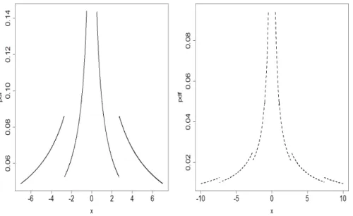
(a) Left: a= 1.1 andb= 0.3. Right: a= 0.9 andb= 0.5
(b) Left: a= 1.1 andb= 0.3. Right: a= 0.9 andb= 0.5
The distribution function G3(x) is given by
G3(x) = d3(a, b)
Z x
−∞
|x|−ae−b⌈|ln|x||⌉dx
=
(
1
2 +d3(a, b)Ix, x >0, 1
2 −d3(a, b)Ix, x <0.
(16)
where
Ix =
Z x
0
y−ae−b⌈|lny|⌉dy
=
(
I1+I2, x >1, I3, 0< x <1.
(17)
withI1, I2 and I3 given respectively in (10), (11) and (12). The density and
distri-bution functions are shown in Figure 3 for some values of the parameters.
3
Generalized Floor Distributions
In this section, the three generalized floor distributions given earlier in [1] are men-tioned. The moments about origin and the distribution functions are obtained for the second and third generalized floor distributions. These results for the first gen-eralized floor distribution are already available in [1].
3.1
Generalized Floor Distribution - I
The density function of the first generalized floor distributionf1(x), as given in [1],
is
f1(x) =C1(a, b)x−ae−b⌊lnx⌋, (18)
forx≥1, a > b+ 1, where
C1(a, b) =
(a−1) eb+1−ea
e−ea . (19)
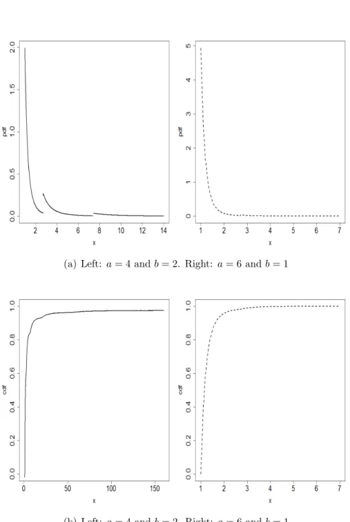
For some values of the parametersaand b,f1(x) and F1(x) are shown in Figure 4.
3.2
Generalized Floor Distribution - II
The second generalized floor distribution, as defined in [1], has the density function given by
f2(x) =C2(a, b)x−ae−b⌊|lnx|⌋, (20)
fora≥0, b >0,1−b < a <1 +b,0< x <∞, where
C2(a, b) =
(a−1) 1−ea−b−1 ea+b−1−1
e2(a−1)−1
(a) Left: a= 0.6 andb= 0.5. Right: a= 0.9 andb= 0.2
(b) Left: a= 0.6 andb= 0.5. Right: a= 0.9 andb= 0.2
(a) Left: a= 4 andb= 2. Right: a= 6 andb= 1
(b) Left: a= 4 andb= 2. Right: a= 6 andb= 1
Ther-th moments about the origin can be easily obtained as
E(Xr) = C2(a, b)
C2(a−r, b)
, (22)
fora−1−b < r < a−1 +b.
The distribution function is given by
F2(x) = C2(a, b)
Z x
0
x−ae−b⌊|lnx|⌋dx
= C2(a, b)
Z lnx
−∞
e−(a−1)ye−b⌊|y|⌋dy.
Following the procedure adopted for the generalized ceiling distribution G2(x),
we obtainF2(x), forx >1, as
F2(x) =
C2(a, b) a−1
e−(1−a)−1
(1−e−(b+1−a)) −
C2(a, b) a−1
e−(a−1)−1
1−e−(b+a−1)⌊lnx⌋
(1−e−(b+a−1))
− C2(a, b)e
−b⌊lnx⌋
a−1
x1−a−e−(a−1)⌊lnx⌋, (23)
forx >1 and 1−b < a <1 +b. Also
F2(x) =
C2(a, b) a−1
(ea−1−1) 1−e−(b−a+1)⌊−lnx⌋
1−e−(b−a+1)
− C2(a, b)e
−b⌊−lnx⌋
a−1
x1−a−e(a−1)⌊−lnx⌋ (24)
for 0< x <1, and b−a+ 1>0. f2(x) and F2(x) are plotted in Figure 5 for some
values of the parametersaand bfor 0< x <∞.
3.3
Generalized Floor Distribution - III
The third generalized floor symmetric distribution defined in [1] has the following form
f3(x) =C3(a, b)|x|−ae−b⌊|lnx|⌋, (25)
fora≥0, b >0,1−b < a <1 +b,−∞< x <∞, where
C3(a, b) =
(a−1) 1−ea−b−1 ea+b−1−1
2 e2(a−1)−1
(eb−1) =
C2(a, b)
2 . (26)
It is easy to obtain ther-th absolute moments as
E(|X|r) = C3(a, b)
C3(a−r, b) =
C2(a, b) C2(a−r, b)
(a) Left: a= 2 andb= 1.2. Right: a= 2 andb= 2.5
(b) Left: a= 2 andb= 1.2. Right: a= 2 andb= 2.5
fora−1−b < r < a−1 +b.
The corresponding distribution function, F3(x), is given by
F3(x) = C3(a, b)
Z x
−∞
|x|−ae−b⌊|lnx|⌋dx
=
(
1
2 +C3(a, b)Ix, x >0, 1
2 −C3(a, b)Ix, x <0.
(28)
where
Ix =
Z x
0
y−ae−b⌊|lny|⌋dy
=
Z lnx
−∞
e−(a−1)ze−b⌊|z|⌋dz. (29)
The values ofIx forx >1 is obtained from the right hand side expression of (23) by omittingC2(a, b) and for 0< x <1 from (24) by omitting C2(a, b). The graphs
(a) Left: a= 1.5 andb= 2. Right: a= 2 andb= 1.4
(b) Left: a= 1.5 andb= 2. Right: a= 2 andb= 1.4
4
Concluding Remarks
The ceiling and the floor distributions may be heavy-tailed distributions. The study of these distributions from ”Regular Variation”, Bingham et al. [2], point of view along with their possible statistical inference analysis and applications will be dis-cussed in a future paper.
Further possible generalizations, their properties and applications will also be subject matter for future research.
ACKNOWLEDGEMENT.P. N. Rathie thanks CAPES, Brazil, for support-ing his Senior National Visitsupport-ing Professorship.
References
[1] J.A.A. Andrade, R.O. Silva and P.N. Rathie. On generalized floor distributions.
13-th Proceedings of the International Conference of the Society of Special Func-tions and ApplicaFunc-tions, 97-106, 2014.
[2] N.H. Bingham, C.M. Goldie and J.L. Tangels. Regular Variation, Vol. 27 of Encyclopedia of Mathematics and Its Applications, Cambridge University Press, Cambridge, 1987.