Localization of a mobile robot based on odometry and natural landmarks using extended kalman filter

(1)

LOCALIZATION OF A MOBILE ROBOT BASED IN ODOMETRY

AND NATURAL LANDMARKS USING EXTENDED KALMAN

FILTER

Andre M. Santana, Anderson A. S. Sousa, Ricardo S. Britto,Pablo J. Alsina, Adelardo A. D. Medeiros

Federal University of Rio Grande do Norte, Natal-RN, Brazil

{andremacedo,abner,rbritto,pablo,adelardo}@dca.ufrn.br

Keywords: Robot Localization, Kalman Filter, Sensor Fusion.

Abstract: This work proposes a localization system for mobile robots using the Extended Kalman Filter. The robot navigates in an known environment where the lines of the floor are used as natural landmarks and identifiqued by using the Hough transform.The prediction phase of the Kalman Filter is implemented using the odometry model of the robot. The update phase directly uses the parameters of the lines detected by the Hough algorithm to correct the robot’s pose.

1 INTRODUCTION

Borenstein et al. have classified the localization methods in two great categories: relative localization methods, which give the robot’s pose relative to the initial one, and absolute localization methods, which indicate the global pose of the robot and do not need previously calculated poses (Borenstein et al., 1997).

As what concerns wheel robots, it is common the use of encoders linked to wheel rotation axes, a tech-nique which is known as odometry (Borenstein et al., 1997). However, the basic idea of odometry is the in-tegration of the mobile information in a determined period of time, what leads to the accumulation of er-rors (Park et al., 1998).

The techniques of absolute localization use land-marks to locate the robot. These landland-marks can be artificial ones, when introduced in the environment aiming at assisting at the localization of the robot, or natural ones, when they can be found in the proper en-vironment. It is important to underline that even the techniques of absolute localization are inaccurate due to noises produced by the manipulated sensors.

Literature shows works using distance measures to natural landmarks (walls, for example) to locate the robot. The obtaining of these measures is generally made with the help of sonar, laser and computational vision (Lizzaralde et al., 2003; Kim and Kim, 2004; Pres et al., 1999).

Bezerra used in his work the lines of the floor composing the environment as natural land-marks (Bezerra, 2004). Kiriy and Buehler, have used extended Kalman Filter to follow a number of artifi-cial landmarks placed in a non-structured way (Kiriy and Buehler, 2002). Launay et al. employed ceiling lamps of a corridor to locate the robot (Launay et al., 2002).

This paper proposes a system enabling to locate a mobile robot in an environment in which the lines of the floor form a bi-dimensional grid. To turn it possible, the lines are identified as natural landmarks and its characteristics, as well as the odometry model of the robot, are incorporated in a Kalman Filter in order to get its pose.

2 THE KALMAN FILTER

The modeling of the Discrete Kalman Filter - DKF presupposes that the system is linear and described by the model of the equations of the system (1):

½_s

t=Atst−1+Btut−1+γt

zt=Ctst+δt

(1)

(2)

matrix of the states;B,n×l, is the coefficient matrix on entry; matrixC,m×n, is the observation matrix;

γ∈Rn_{represents the vector of the noises to the} pro-cess and δ∈Rm the vector of measurement errors. Indexes t andt−1 represent the present and the pre-vious instants of time.

The Filter operates in prediction-actualization mode, taking into account the statistical proprieties of noise. An internal model of the system is used to updating, while a retro-alimentation scheme accom-plishes the measurements. The phases of prediction and actualization to DKF can be described by the sys-tems (2) and (3) respectively.

( ¯

µt=Atµt−1+Btut−1

¯

Σt=AtΣt−1ATt +Rt

(2)

  

 

Kt=Σ¯tCtT(CtΣ¯tCTt +Qt)−1 µt=µ¯t+Kt(zt−Ctµ¯t)

Σt= (I−KtCt)Σ¯t

(3)

The Kalman Filter represents the vector of the statesst by its meanµt and co-varianceΣt. Matrixes

R, n×n, and Q, l×l, are the matrixes of the co-variance of the noises of the process (γ) and measure-ment (δ) respectively, and matrixK,n×m, represents the prot of the system.

A derivation of the Kalman Filter applied to non-linear systems is the Extended Kalman Filter - EKF. The idea of the EKF is to linearize the functions around the current estimation using the partial deriva-tives of the process and of the measuring functions to calculate the estimations, even in the face of non-linear relations. The model of the system to EKF is given by the system (4):

½_s

t=g(ut−1,st−1) +γt

zt=h(st) +δt

(4)

in whichg(ut−1,st−1)is a non-linear function

repre-senting the model of the system, andh(st)is a non-linear function representing the model of the measure-ments.

Their prediction and actualization phases can be obtained by the systems of equations (5) and (6) re-spectively.

( ¯

µt=g(ut−1,µt−1)

¯

Σt=GtΣt−1GtT+Rt

(5)

  

 

Kt=Σ¯tHTt (HtΣ¯tHTt +Qt)−1 µt=µ¯t+Kt(zt−h(µ¯t))

Σt= (I−KtHt)Σ¯t

(6)

The matrixG,n×n, is the jacobian term linearizes the model andH,l×nis the jacobian term linearizes

the measuring vector. Such matrixes are defined by the equations (7) e (8).

Gt=

∂g(ut−1,st−1)

∂st−1

(7)

Ht=

∂h(s_t)

∂st

(8)

Next we will describe the modeling of the prob-lem, as well as the definition of the matrixes which will be employed in the Kalman Filter.

3 MODELING

3.1 Prediction phase: Odometer model

of the robots movement

A classic method used to calculate the pose of a robot is the odometry. This method uses sensors, optical encoders, for example, which measure the rotation of the robot’s wheels. Using the cinematic model of the robot, its pose is calculated by means of the integra-tion of its movements from a referential axis.

As encoders are sensors, normally their reading would be implemented in the actualization phase of the Kalman Filter, not in the prediction phase. Thrun et al. propose that odometer information does not function as sensorial measurements; rather they sug-gest incorporating them to the robot’s model (Thrun et al., 2005).

In order that this proposal is implemented, one must use a robot’s cinematic model considering the angular displacements of the wheels as signal that the system is entering in the prediction phase of the Kalman Filter.

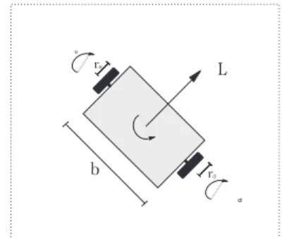
Consider a robot with diferential drive in which the control signals applied and its actuators are not tension, instead angular displacement, according to Figure 1.

D qd

D L

D q

b D qe

re

rd

(3)

With this idea, and supposing that speeds are con-stant in the sampling period, one can determine the geometric model of the robot’s movement(system 9).

          

         

xt=xt−1+

∆L

∆θ[sin(θt−1+∆θ)−sin(θt−1)]

yt=yt−1−

∆L

∆θ[cos(θt−1+∆θ)−cos(θt−1)] θt=θt−1+∆θ

(9)

The turn easier the readability of the system (9) representing the odometry model of the robot, two auxiliary variables have been employed∆Land∆θ

½_∆_L_{= (}_∆θ

drd+∆θere)/2

∆θ= (∆θdrd−∆θere)/b

(10)

in which∆θdis the reading of the right encoder and functions relatively the robot by means of the angular displacement of the right wheel;∆θeis the reading of the left encoder and functions as a displacement ap-plied to the left wheel;brepresents the distance from wheel to wheel of the robot;rdandreare the spokes of the right and the left wheels respectively.

It is important to emphasize that in real applica-tions the angular displacement effectively realized by the right wheel differs of that measured by the en-coder. Besides that, the supposition that the speeds are constant in the sampling period, which has been used to obtain the model 9, is not always true. Hence, there are differences between the ” angular displace-ments of the wheels (∆θˆde∆θˆe) and those ones mea-sured by the encoders (∆θd e∆θe). This difference will be modeled by a Gaussian noise, according to system (11).

(

∆θˆd=∆θd+εd

∆θˆe=∆θe+εe

(11)

It is known that odometry possesses accumulative error. Therefore, the noisesεdandεedo not possess constant variance. It is presumed that these noises present a proportional standard deviation to the mod-ule of the measured displacement.

With these new considerations, system (9) is now represented by system (12):

           

          

xt=xt−1+

∆Lˆ

∆θˆ[sin(θt−1+∆

ˆ

θ)−sin(θt−1)]

yt=yt−1−

∆Lˆ

∆_θˆ[cos(θt−1+∆θˆ)−cos(θt−1)]

θt=θt−1+∆θˆ

(12)

in which (

∆Lˆ= (∆θˆdrd+∆θˆere)/2

∆θˆ= (∆θˆdrd−∆θˆere)/b

(13)

One should observe that this model can not be used when ∆θˆ =0. When it occurs, one uses an odometry module simpler than a robot (system 14), obtained from the limit of system 12 when∆_θˆ_→_0.

  

 

xt=xt−1+∆Lˆcos(θt−1)

yt=yt−1+∆Lˆsin(θt−1)

θt=θt−1

(14)

Thrun’s idea implies a difference as what concerns system (4), because the noise is not audible; rather, it is incorporated to the function which describes the model, as system (15) shows:

½_s

t=p(ut−1,st−1,εt)

zt=h(st) +δt

(15)

in whichεt= [εdεe]Tis the noise vector connected to odometry.

It is necessary, however, to bring about a change in the prediction phase of the system (6) resulting in the system (16) equations:

( ¯

µt=µt−1+p(ut−1,µt−1,0)

¯

Σt=GtΣt−1GtT+VtMtVTt

(16)

in which M, l×l, is the co-variance matrix of the noise sensors(ε)andV,n×m, is the jacobian map-ping the sensor noise to the space of state. Matrix V is defined by the equation (17).

Vt=

∂p(ut−1,st−1,0)

∂ut−1

(17)

(4)

ma-trixes used by the Kalman Filter, we have:

G=





1 0 g13

0 1 g23

0 0 1



, onde (18)

(19)

g13=

∆Lˆ

∆_θˆ[cos(θt−1+∆θˆ)−cos(θt−1)]

g23=

∆_Lˆ

∆θˆ[sin(θt−1+∆

ˆ

θ)−sin(θt−1)]

V=





v11 v12

v21 v22

rd/b −re/b 

, onde (20)

(21) v11=k1 cos(k2)−k3[sin(k2)−sin(θt−1)]

v12=−k1 cos(k2) +k3[sin(k2)−sin(θt−1)]

v21=k1 sin(k2)−k3[−cos(k2) +cos(θt−1)]

v22=−k1 sin(k2) +k3[−cos(k2) +cos(θt−1)]

M=

µ

(α1|∆θˆd|)2 0

0 (α2|∆θˆe|)2

¶

(22)

Elementsm11 andm22 in the equation (22)

rep-resent the fact that the standard deviations ofεd and

εeare proportional to the module of the angular dis-placement. The variablesk1,k2 andk3 are given by system (23), consideringrd=re=r.

         

        

k1= r(∆θˆd+∆θˆe)

b(∆θˆd−∆θˆe)

k2=θt−1+

r(∆θˆd−∆θˆe) b

k3= b∆θˆe

2(r(∆_θˆ_d₋_∆_θˆ_e₎_/b)2

(23)

3.2 Update Phase: Sensor Model for

Detecting Natural Landmarks

In this work we will use as natural landmarks a set of straight lines formed by the grooves of the floor in the environment where the robot will navigate be-cause, besides being already available in the referred environment, they are also very common in the real world.

Due to the choice of the straight lines as land-marks, the technique adopted to identify them was the Hough transform. This kind of transform is a method employed to identify inside a digital image a class of

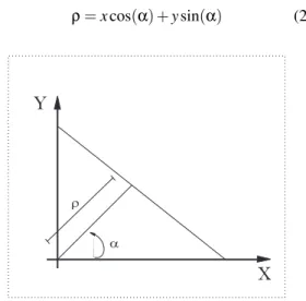
geometric forms which can be represented by a para-metric curve (Gonzales, 2000). As what concerns the straight lines, a mapping is provided between the Cartesian space(X,Y)and the space of the parame-ters(ρ,α)where the straight line is defined.

Hough defines a straight line using its common representation, as equation (24) shows, in which pa-rameterρrepresents the length of the vector andαthe angle this vector forms with axis X. Figure 2 shows the geometric representation of these parameters.

ρ=xcos(α) +ysin(α) (24)

a r

X

Y

Figure 2: Parameters of the Hough.

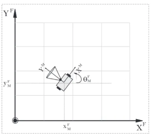
The system discussed in this paper is based in a robot with differential drive, possessing a rm and sta-ble camera embedded in its structure, as in Figure 3. The idea is to use information obtained directly on the image processing(ρ,α)in the actualization phase of an Extended Kalman Filter to calculate the robot’s pose. Thereof, one must deduct the sensor model (that is, the image processor) in function of the variables of state.

(5)

Y

x_MF

y_MF

F

XF X

M

Y

M

q_MF

Figure 4: System of Coordinates.

Robot navigates an environment in which the po-sition of the straight lines of the world (αF_, _ρF_{) is} known and, at each step, it identifies the descriptors of the straight lines contained in the image (αM_,_ρM₎ us-ing image processus-ing and the parameters of the cam-era gauging.

Figure 4 illustrates the systems of steady{F}and mobile{M}coordination used to mathematic deduc-tion of the sensor model. The point(xF_M,yF_M)is the coordinate of origin of the mobile system mapped in the system of steady and mobile coordinates, while variableθF

M represents the rotation angle of the sys-tem of mobile coordinates.

Our point of departure is a simple change map-ping a point in the system de mobile{M}coordinates for the system of steady{F} coordinates, as in sys-tem (25).

(

xF=cos(θMF)xM−sin(θMF)yM+xFM yF=sin(θM

F)xM+cos(θMF)yM+yFM

(25)

Using an equation (24) and considering the system of steady{F}coordinates, we have:

ρF₌_xF_cos₍_αF_{) +}_yF_sin₍_αF₎ ₍₂₆₎ Also using the definition of system (24), but now considering the system of mobile{M} coordinates, we have:

ρM₌_xM_cos₍_αM_{) +}_yM_sin₍_αM₎ ₍₂₇₎ Replacing (25) in (26) and doing the necessary equivalences with system (27), we can obtain sys-tem (28), which represents the sensor module to be used in the filter.

(

αM=αF−θFM

ρM₌_ρF₋_xF

Mcos(αF)−yFMsin(αF)

(28)

In this system,αF_and_ρF_{are given, because they} represent the description of the map landmark, which is supposedly known. The equations express the re-lations among the returned information (αF_,_ρF_{) and} the height that one wants to estimate (xM_F,yM_F,θM

F). One should note that there is a straight relation among these variables (xM

F,yMF,θMF) and the robot’s pose (xR,yR,θR), which is given by system 29.

   

  

xR=xMF yR=yM_F

θR=θMF +

π

2

(29)

The model of system 28 is incorporated to the Kalman Filter through matrix H (equation 8), given by equation 30.

H=

µ

−cos(θF

M) −sin(θFM) 0

0 0 −1

¶

(30)

4 RESULTS

The situations presented here have been obtained by simulation. We tried to use the noise measure of the sensors consistent to reality. For that, it has been embedded to encoders a noise which standard devi-ation is proportional to the amount of read pulses. In the identification of the parameters of the straight lines ρ and α, the standard deviation of noise also obeys a proportion which is ruled by the size that the straight line occupies in the image.

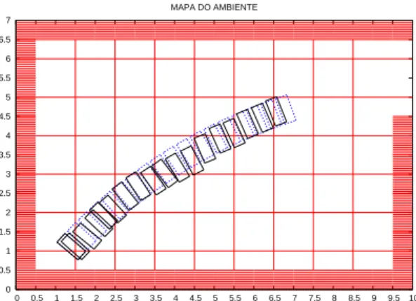
In the Figures, the hatched rectangle represents the robot’s real pose, while the continuous rectangle, the calculated pose.

Figure 5 presents the result of the localization sys-tem using only odometry.

Another localization system largely used has also been implemented: the localization system using ge-ometric correction. In this system, at each step the straight lines are identified and used to calculate the robot’s pose using trigonometry. When there are no straight lines, the correction is made by odome-try(Figure 6).

Finally, in Figure 7 is shown the result of the pose calculation using the fusion of the data of odometry and of the landmark detection by EKF.

(6)

0 0.5 1 1.5 2 2.5 3 3.5 4 4.5 5 5.5 6 6.5 7

REFERENCES

Bezerra, C. G. (2004). Localizao de um rob mvel usando odometria e marcos naturais. Master’s thesis, Univer-sidade Federal do Rio Grande do Norte, UFRN, Natal, RN.
Borenstein, J., Everett, H., Feng, L., and Wehe, D. (1997). Mobile robot positioning: Sensors and techniques. Journal of Robotic Systems, 14(4):231–249.
Gonzales, R. C. (2000). Processamento de Imagens Digi-tais. Edgard Blucher.
Kim, S. and Kim, Y. (2004). Robot localization using ultra-sonic sensors. Proccedings of the 2004 IEEE/RSJ In-ternational Conference on Inteligent Robots and Sys-tems, Sendal, Japan.
Kiriy, E. and Buehler, M. (2002). Three-state extended kalman filter for mobile robot localization. Report Centre for Intelligent Machines - CIM,McGill Univer-sity.
Launay, F., Ohya, A., and Yuta, S. (2002). A corridors lights based navigation system including path definition us-ing a topologically corrected map for indor mobile robots. Proceedings IEEE International Conference on Robotics and Automation, pp.3918-3923.
Lizzaralde, F., Nunes, E., Hsu, L., and J.T., W. (2003). Mo-bile robot navigation using sensor fusion. Procced-ings of the 2003 IEEE International Conference on Robotics and Automation, Taipei, Taiwan.
Park, K. C., Chung, D., Chung, H., and Lee, J. G. (1998). Dead reckoning navigation mobile robot using an in-direct kalman filter. Conference on Multi-sensor fu-sion and Integration for Intelliget Systems, 9(3):107-118.
Pres, J., Catellanos, J., Montiel, J., Neira, J., and Tards, J. (1999). Continuous mobile robot localization: Vision
vs. laser. Proccedings of the 1999 IEEE International Conference on Robotic and Automation.
Thrun, S., Burgard, W., and Fox, D. (2005). Probabilistic