Ensaios Econômicos
Escola de
Pós-Graduação
em Economia
da Fundação
Getulio Vargas
N◦ 781 ISSN 0104-8910
Taxation of Couples: a Mirrleesian Approach
for Non-Unitary Households*
Carlos E. da Costa, Lucas A. de Lima
Os artigos publicados são de inteira responsabilidade de seus autores. As
opiniões neles emitidas não exprimem, necessariamente, o ponto de vista da
Fundação Getulio Vargas.
ESCOLA DE PÓS-GRADUAÇÃO EM ECONOMIA Diretor Geral: Rubens Penha Cysne
Vice-Diretor: Aloisio Araujo
Diretor de Ensino: Carlos Eugênio da Costa Diretor de Pesquisa: Humberto Moreira
Vice-Diretores de Graduação: André Arruda Villela & Luis Henrique Bertolino Braido
E. da Costa, Carlos
Taxation of Couples: a Mirrleesian Approach for
Non-Unitary Households*/ Carlos E. da Costa, Lucas A. de Lima – Rio de Janeiro : FGV,EPGE, 2016
64p. - (Ensaios Econômicos; 781)
Inclui bibliografia.
Taxation of Couples: a Mirrleesian Approach
for Non-Unitary Households
∗
Carlos E. da Costa
EPGE-FGVLucas A. de Lima
HarvardAugust 2, 2016
Abstract
Optimal tax theory in theMirrlees’ (1971) tradition implicitly relies on the assumption that all agents are single or that couples may be treated as individuals, despite accumulating evidence against this view of house-hold behavior. We consider an economy where agents may either be sin-gle or married, in which case choices result from Nash bargaining between spouses. In such an environment, tax schedules must play the double role of: i) defining households’ objective functions through their impact on threat points, and; ii)inducing the desired allocations as optimal choices for households given these objectives. We find that thetaxation principle, which asserts that there is no loss in relying on tax schedules is not valid here: there are constrained efficient allocations which cannot be mented via taxes. More sophisticated mechanisms expand the set of imple-mentable allocations by: i)aligning the households’ and planner’s objec-tives; ii)manipulating taxable income elasticities, and; iii)freeing the de-sign of singles’ tax schedules from its consequences on households’ objec-tives. Keywords:Mechanism Design; Collective Households; Nash-bargain. JEL Codes:D13; H21; H31.
∗
I Introduction
The use of labor income tax schedules to advance societies’ distributive goals is grounded on sound theoretical basis guaranteeing that relying on such in-struments is without loss. Whereas the revelation principle — Dasgupta et al.
(1979); Myerson(1979); Harris and Townsend (1981) — proves that the set of allocations that can be implemented is not constrained by the use of a direct mechanism, the taxation principle —Hammond(1979,1987) — guarantees that there is always a tax schedule that induces the allocations implemented by a di-rect mechanism. Put together these results imply that one can do no better than using a tax schedule.
In the context of optimal tax theory both the revelation and the taxation principles have been proved under the assumption that either everyone is sin-gle or couples that can be treated as if they were individuals.1 Of course we all
recognize that most adults are not single. Moreover, recent advances in family economics suggest that the conditions under which couples may be treated as individuals are very stringent and not likely to be verified in practice. The pur-pose of this paper is to assess whether the extension of results from optimal tax theory from singles to couples is granted when these conditions are not met.
We modify Mirrlees’ (1971) economy by taking the non-unitary nature of couples seriously. The informational structure inMirrlees(1971) is modified by the assumption that spouses know each other’s productivities, which are oth-erwise private information. Finally, married agents decide through a bargain procedure that satisfyNash’s (1950) axioms. In agreement, spouses maximize a Nash product which threat points are determined by the equilibrium of a non-cooperative disagreement game that depends on the very institutional setting under which household choices are made.
The first question we ask is whether one may still rely on the revelation prin-ciple to characterize the set of implementable allocations. Our answer is yes: any implementable allocation may be truthfully implemented by a Direct Mech-anism – DM. For singles, nothing new: agents reports their productivity and an outcome function maps announcements into transactions. As for couples, at the moment a married agent ’communicates with the mechanism’ he (she)
1The expression ’be treated as if’ is used to represent both the positive assessment regarding
knows his (her) own productivity, his (her) spouses’ productivity and whether the household has reached an agreement or not. This informational structure imposes the definition of a married agent’s type, a vector comprised of: i) his (her) productivity;ii)his (her) spouses’ productivity, and;iii)whether the cou-ple is in agreement or disagreement.2 An outcome maps both spouses reports
about their types into transactions.
If households’ objectives were invariant to policy, all the results in Ham-mond(1979,1987);Guesnerie(1998) regarding the taxation principle would still be valid here. In fact, very simple mechanisms for which each agent is only asked his (her) productivity would suffice. What makes the non-unitary setting special is the fact that threat points are as much determined by the tax sched-ules as the choices made under the ordering represented by the Nash prod-uct. Hence, the equivalence between two institutions depends not only on their ability to replicate choicesconditional on threat points, but also on their capac-ity to generate the same threat points as equilibrium utilities for households in disagreement.
The taxation principle fails, i.e., tax schedules cannot in general implement an arbitrary incentive-feasible allocation, because a single schedule must play the double role of implementing the desired allocation for given household ob-jectives and inducing those obob-jectives. By contrast, by allowing different choice
sets for couples whether in agreement or disagreement alternative institutions/mechanism generate some separation between the two instruments.
The logic of our results can be grasped from an optimal taxation perspective as follows. When one perturbs a tax schedule, the welfare impact is very closely related to the mechanical impact on tax revenues due to a direct application of the envelope theorem. With dissonance, this needs not to be true: behavioral responses in the form of redistribution across spouses have first order effect on welfare when the marginal value of income differ between spouses from the planner’s perspective. This is dissonance, as defined byApps and Rees(1988), in a nutshell. If threat points can be manipulated, this may be useful to align the planner’s objective with that of households.3
2Throughout the paper we use the terms agreement and disagreement to define,
respec-tively, the state under which an agreement to cooperate and split the surplus of marriage has been reached, and the one for which no such agreement has yet been reached and decisions are made in non-cooperatively.
3This is most apparent when utility is transferable, the case studied byda Costa and Diniz
With regards to behavioral responses, it is important to recall that policy elasticities, e.g.,Hendren(2016), are not structural parameters. In the context of household taxation, elasticities are bound to depend on threat points therefore being choice parameters. As inKopczuk and Slemrod(2002), elasticities should be optimally chosen.
The rest of the paper is organized as follows. After a brief related literature overview, SectionIIpresents the environment. In SectionVIwe define a Direct Mechanism and prove that the revelation principle is valid in this non-unitary setting. SectionVIIstudies tax systems here taken as collections of tax sched-ules. Finally, in SectionVIII.1we explains how the manipulation of threat points made possible by a DM expands the set of allocations which may be imple-mented by a tax system. SectionIXconcludes.
I.1 Literature Review
In its essence the paper addresses the use of mechanism design to a group deci-sions problem motivated by a modern view of household decideci-sions. It belongs in both the optimal taxation and the family economics literature. To under-stand the current state of optimal taxation of households, one must start with the pioneering work ofBoskin and Sheshinski(1983) who invited the profession to take seriously the fact that most individuals in society interact directly with their spouses in ways that have potentially important consequences for tax de-sign. They proceeded by adopting what is nowadays referred to as the unitary approach to household behavior. Under this approach couples are modeled es-sentially as a single agent with multiple, perfectly assignable, choices of effort.
If couples may be treated as single agents, then the optimal taxation problem can be solved by noting that: i)a direct incentive feasible mechanism is without loss (i.e., the revelation principle applies), and;ii)the allocations implemented by the mechanism are the same as the allocations induced by a suitably defined tax schedule (i.e., the taxation principle applies).
The problem is that, however tractable one may find the unitary approach, its poor adherence to the data — e.g.,Browning and Chiappori(1998) — has led to a recurring questioning of its usefulness to policy design. Indeed, this failure to describe actual choices made by couples has already crossed the boundaries of academic to influence actual policy design.4
pro-The decline of this unitary view of the household is followed by the emer-gence of an alternative, collective view of household behavior. It agrees with the unitary approach with respect to the incentives spouses have to choose effi-ciently but recognizes the conflicting opinions regarding which efficient choices to make.
The goal of our paper is to bring optimal tax theory to terms with the novel findings in Family Economics by providing analogues of (i) and (ii) for house-holds which behavior is better approximated by the collective model.
In a broader sense, we refer to collective models as those, axiomatic in na-ture, which only assume that households can achieve efficient outcomes with-out specifying the process leading to such with-outcomes — see the discussion in
Chiappori and Mazzocco (2015). At this level of generality, however, not very much can be said from a normative perspective. We adopt the early formula-tion of Manser and Brown (1980);McElroy and Horney(1981) which assumes that couples decisions are made through Nash bargaining. Central to our anal-ysis is, therefore, the impact of policies on threat points.5
The literature has considered two types of threat points: i) external, usu-ally modeled as the utility of being single, and; ii) internal, given by the utility attained within marriage if cooperation ceases. ’External’ threat points were used in the pioneering works ofManser and Brown(1980);McElroy and Horney
(1981). Internal threat points are important if one is to account for changes in household behavior that result from factors that only affect spouses while mar-ried, as in the ’separate spheres’ model ofLundberg and Pollak(1993).
From a purely theoretical perspective,Binmore(1985);Binmore et al.(1989) make the point that outside options do not define threat points. They, instead, provide bounds for utilities that can arise in any bargain. Application of this idea to household economics –Bergstrom(1996) – leads to the idea that it is the util-ity attained when cooperation ceases and choice are made non-cooperatively that ultimately defines threat points.
Our work also has implications for the perturbation methods (or elasticities approach) developed by Piketty (1997); Dahlby (1998); Saez(2001) which has
grams which design explicitly acknowledges the failure of one of the well known properties of unitary models: income pooling.
5Since the axiomatic solution to a Nash bargain imposes efficiency, these models are
become the standard for optimal labor income taxation. This approach for the taxation of couples is very useful if the unitary approach may be used given the multi-dimensional nature of the screening problem — e.g.,Kleven et al.(2009).6
When (i) and (ii) apply one may either solve the mechanism design problem and use the resulting allocations to build the optimal tax schedule, or start from a candidate optimum schedule and show use local changes to derive necessary conditions for an optimum.7 Under the latter approach one needs not to rely on
the simplifying assumptions adopted byMirrlees(1971), which are very hard to hold in practice when we consider the underlying structure of the household problem. More specifically, the uni-dimensional nature of the problem that al-lowed single-crossing to arise under very weak assumptions on preferences in the case of singles is lost in the case of couples.
Although our results show that an optimal tax schedule need not implement the optimal allocation, we may still ask whether the elasticities approach can be used to study the somewhat less ambitious goal of deriving optimal tax sys-tems. By using carefully chosen filing options the perturbations and elasticities remain meaningful, which will not be the case if one relies on simple tax sys-tems. Moreover, policy elasticities are not structural parameters.8 Instead they
are determined by the hole structure of the economy and should be optimally chosen as inSlemrod and Kopczuk(2002).
II Environment
The economy we describe is an extension ofMirrlees’ (1971) to a setting where we allow a subset of the agents to be married.
A continuum of individuals, of two different genders,i = f, m, have prefer-ences defined over consumption,c, and leisure, l, which may depend on their gender, but are otherwise identical across individuals. Preferences for a gen-deriagent may be represented by the utility functionui(c,l), increasing in both variables and strictly quasi-concave.9
6Such an application of variational methods is found inGolosov et al.(2014).
7The main drawback is, of course, that it does not offer a method for actually finding the
optimum.
8An account of the nature of policy elasticities is explained inHendren(2016). Our results
show that they vary for the same principal tax schedule, if we vary the filing option.
9u
i(·)is also the cardinal representation that will be relevant for the Nash bargaining
As inMirrlees(1971), agents differ with respect to their labor market produc-tivity,θi ∈Θ,i=f, m.
Agents may be single or married. For notation simplicity only we shall re-strict the analysis to couples comprised of agents of different genders. A couple is, therefore, identified by a pair of productivities: θf for the wife andθm for the
husband. We useη= (θf, θf)for brevity.
The distribution of singles of gender i is given by a measure µi
s in Θ. The
distribution of couples is given by a measureµcinΘ2. We assume that these are
known (by the planner at least) distributions which are held fixed as we change policies.
Finally, technology is represented by a transformation function,G :Z2 7→R
that assigns a non-positive value for feasible allocations and a positive value for unfeasible ones.
Informational Structure The information structure is as follows. An agent’s type is his or her private information. For singles, this means that a gender i
agent is the only one to know its type,θi.
For married agents we assume that each spouse i — for i = f, m — in a coupleη = (θf, θm)knows not only his or her productivityθi, but also his or her
spouses’ productivity, θj — fori, j = f, m. I.e., both the husband and the wife
and noone else knowsη. This assumption about the informational structure of an economy with households is consistent with the type of efficient decisions implied by the collective model in general and the Nash bargaining model in particular.10
Transactions The consumption bundle(c,l)of an agent is observed by noone but the agent him or herself, if the agent is single. It is observed by both spouses when the agent is married. What is observed by everyone are the transactions made by single agents and household. A tax schedule may only, as a conse-quence, depend on transactions.11
10The idea that households can efficiently bargain for instance may not be reasonable if
spouses have private information with respect to each other.
11For a direct mechanism, the inclusion of obedience constraints allows one to write in terms
Singles A transaction is a vectorz ∈ Z ⊂ R2, whereZ is a compact
sub-set of R2, which describes everything an agents buys as positive entries and
everything he or she sells as negative entries. All agents are assumed to have the same endowment,(0,1), of consumption good and time. A transaction vec-tor z = (c,−n), describes the amount of hours, n, the agent supplies and the amount of consumption goods he or she acquires in the market,c. Given the en-dowment(0,1)the bundles attainable by a typeθiagent are(c,l)≤(c,1−n/θi).
Because utility is strictly increasing in bothcandl, a single agent will always choose(c,l) = (c,1−n/θi). Hence, there is one to one mapping between transac-tions,z, and consumption bundles,(c,l), which allows us to define the induced preferences over the setZ,θi. We writez ∈ Z to define transactions such that
z θi zfor allz ∈ Z, allθi,i=f, m, which we assume to exist.
Couples For couples, define z = (zf, zm) ∈ Z2, wherezf are the
transac-tions made by the wife andzmthose made by the husband.
The mapping from transactions to consumption bundles for couples is more involved than those for singles. We define a functionFa : Z2×Θ2 → 2X which
maps the transaction realized by a couple into sets of feasible pairs of bundles that can be consumed by this couple. Embedded in this function are not only the material gains from marriage but also all relevant transferability restrictions. For example, if a η = (θf, θm)chooses transactionz = (cf,−nf, cm,−nm), then
the wife must be enjoying leisurelf ≥1−nf/θfand the husband,lm ≥1−nm/θm.
As for consumption goods, we may allow for gains of scale by assuming that all consumption pairs(cf,cm)such thatcf+cm ≤α(cf+cm)forα >1are attainable.
We write
Fa(z, η) :=
((cf,lf),(cm,lm)) ;cf +cm ≤α[cf +cm] ;lf ≤1− nf θf
;lm ≤1− nm θm
.
Note that consumption is transferable across agents, hence non-assignable, while leisure is not. Transactions are not, therefore, directly mapped into utilities. In-stead, for any givenz = (zf, zm)and anyη, a (conditional) utility possibility set
II.1 Households’ Decision Process
Couples’ decisions are the outcome of a bargain which solution satisfies a vari-ation ofNash’s (1950) axioms advanced byZambrano(2016) to account for pos-sible non-convexities of utility possibility sets.12 The Nash bargaining solution
is formulated in terms of a set o feasible utility pairs that households can attain by cooperating and a disagreement pair(¯uf,u¯m)that represents the utility that
spouses obtain if an agreement is not reached.
Of course, a crucial question that needs to be addressed in any applica-tion is what these disagreement utilities are. There are potentially many can-didates depending on the application we are considering, and in family eco-nomics different possibilities have been considered. The early works ofManser and Brown (1980); McElroy and Horney (1981) took divorce to be the relevant threat points whereasLundberg and Pollak(1993) pioneered the used of ’inter-nal’ threat points as the utility attained as spouses cannot reach a disagreement and choose non-cooperatively. This is also the view sponsored byBergstrom
(1996) who uses the results inBinmore(1985) to argue in favor of ’burning toasts’ threat points, i.e., utilities attained by spouses as agreement is not reached and cooperation ceases. Outside options, here interpreted as the utilities attained at divorce, define lower bounds on utilities that agents can be assigned, but oth-erwise play no role in the definition of the outcome. InBinmore et al.(1989), where laboratory experiments are used to assess which of these threat points are more relevant, outside options are referred to as ’breakdown points’ whereas the utilities attained if bargaining continues without an agreement are called ’impasse point’. It is important however to mention that in Binmore (1985),
Binmore et al.(1989) andBergstrom(1996) both the breakdown points and the impasse points are givens, whereas a central concern in household economics is how changes in the environment affect these threat points.
Understanding how the institutional design affect threat points is the essence of our analysis. Toward this end, we shall define two different states in which a marriage can be: agreement and disagreement. Note that this, too is private information. Moreover, this disagreement state does not happen in equilib-rium. Spouses do however understand and anticipate clearly what would
hap-12Zambrano’s (2016) ’preference for symmetry’ substitutes forNash’s (1950) symmetry axiom.
pen were they not able to reach an agreement.
A couple is in agreement if spouses have been able to settle their differences, having thus agreed on how to rank transactions and on how to allocate the prod-uct of such transactions between themselves. In this case, spouses maximize the Nash product,
(uf(cf,lf)−u¯f) (um(cm,lm)−u¯m), (1)
whereu¯f andu¯mare the threat points with respect to which choices are made.
In disagreement spouses play a non-cooperative game that defines these threat points. Contrary toBergstrom(1996) andBinmore(1985), for that matter, outside options play in our setting a role in disagreement. We assume that rever-sion to singlehood is possible at any moment. Hence, these breakdown points define lower bounds on threat points. As in Bergstrom(1996); Binmore et al.
(1989);Binmore (1985) outside options do not per se define the threat points. Yet, because we provide each spouse with the ability to unilaterally force the dissolution of marriage at any stage, they define lower bounds for the disagree-ment game. A straightforward consequence is that outside options never bind in agreement.
III Heuristics for Main Results
Final consumption of goods and leisure are not observed. Hence, it cannot be the base for taxation. Instead, tax schedules are imposed on transactions. In the case of singles, this is of little consequence, since strong monotonicity in prefer-ences guarantee a one to one mapping from transactions to final consumption. For couples matters are not so simple.
Our departure point is an optimal tax system which defines for a single agent of gender i, i = f, mthe set of feasible transactions {zi ∈Z|ψi(zi)≤0}, in the
form of a budget set induced by the optimal tax schedule. Similarly for cou-ples,{z ∈Z2|ψ(z)≤0}, whereψ(·)plays for couples the role thatψi(·)play for
genderisingles.
In the case of multi-persons households, not all goods are assignable. In par-ticular, the planner does not observe how the consumption goods, acquired by a couple, cf +cm, are split between spouses. As a consequence, transactions
Which point in the set is chosen, then depends on a bargain which solution we assume to satisfy the axioms proposed byNash(1950).
Threat points must be defined for the household objective, the Nash prod-uct, to be determined. This happens as follows. Couples maybe in one of two al-ternative states: agreement or disagreement. In agreement, spouses act cooper-atively and maximize the Nash product. In disagreement, i.e., if they have failed to reach common grounds to make a choice, spouses play a non-cooperative game which defines the threat points. We model this latter stage as follows.
For each coupleηletΦbe a mapping from transactionszto a pair of utilities
(¯uf,u¯m), in the interior of set Uz(η), Φ(z, η) = (¯uf,u¯m) ∈ U˚z(η). We shall have
more to say about this mapping later. For now, one need only recognize that it is through this function that threat points are determined.
It is important to note that threat points depend only on transactions that are chosen at the Nash equilibrium for the disagreement game. They do not depend on the specific way under which these transactions are reached. It is this feature that allows us to compare threat points across different institutional settings.
Let us, then compare outcomes for two different institutions. First, is the optimal tax system previously described.
Second, is a general mechanism
M ≡ {Σsi,Σ c
i}i=f,m,{g s
i(·)}i=f,m,g c
(·,·),
where (Σs
i)i=f,m are message spaces for single agents, Σci message spaces for
married agents, (gs
i(·))i=f,m outcome functions for singles and gc(·,·)outcome
function for couples.
Under a tax system agents choose transactions directly, and we letZc
Ψdenote
the set of all transactions that are feasible for couples under the tax system, i.e.,
Zc
Ψ :={z ∈Z2|ψ(z)≤0}. Similar sets are defined for singles of either gender.
Under a mechanism, transactions are chosen indirectly through the mes-sages sent to the center. We define the set of transactions available to any house-hold underMasZc
M :={z ∈Z2|∃(σf, σm)∈Σf ×Σmsuch thatgc(σf, σm) = z}.
For households are in agreement, ifZc
M=ZΨc, the same choices will be made
The question is whether threat points coincided for the two institutions. The answer is, not necessarily. In the non-cooperative game, different mechanisms will be associated with different strategy spaces. Under a tax schedule, a hus-band chooses his transactions taking his wife’s transactions as given, whereas under a mechanism he chooses his announcement taking his wife’s announce-ments as given. Hence, even if Zc
M = ZΨc, different equilibrium transactions
will, in general result. Different threat points may, therefore, arise in the dis-agreement game.
Hence, given an optimal tax system, it may still be possible to improve upon the resulting allocation if one is able to change threat points in useful direc-tions.13 Of course we have no reason to restrict reforms to those that preserve
the set of attainable transactions. In fact we next present two examples of how threat points may improve upon a given allocation. In our second example, threat points are used to break a couple’ indifference between two transactions. A typical reform would use the fact that the household is no longer indifferent between the two transactions to redesign the set of available transactions. For our first example, however, we consider a reform that preserves the set of avail-able transactions.
Consider an economy in which, for all households, utility is transferable across spouses. The convenient aspect of such example is that households choose transactions that maximize their surplus regardless of how it will later be split — see Lemma 2. Letli = 1−ni/θi fori = f, m., denote the amount of leisure
that spouseiwhose productivity isθi consumes. Then, given transactionsz = (cf,−nf, cm,−nm), the household solves
max
cf
cf +h
1− nf
θf
−u¯f cf +cm−cf +h
1− nm
θm
−u¯m
,
where(¯uf,u¯m), are the relevant threat points andh(·)is an increasing concave
function that captures the utility of leisure.
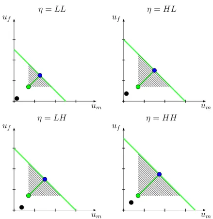
Consider a planner whose objective is to maximize the average logarithm of agents utilities. The concave social welfare function is needed for this quasi-linear example. In this case, the household and the planner objectives are aligned if and only if u¯f − u¯m = 0. If under the optimal tax schedule z maximizes
13A simple example of such reforms is found inda Costa and Diniz(2015), in the context of
Singles’ utilities threat points Alternative threat points
um uf
um uf
Figure 1:Aligning ObjectivesThe panel in the left displays the set of individually rational utility pairs, when the threat point — green dot — is induced by the tax schedule in place. The blue dot denotes optimal choice for the couple. If the planner is able to induce a different threat point — green dot in the right panel — a new choice distribution of utilities is induced for the same transactions.
the household’s surplus, therefore, inducing this transaction as the household’s choice, then we can represent the utility possibility set for as in Figure1. The op-timal choice is given by a straight 45 degrees line from(¯uf,u¯m)to the frontier of
the utility possibility set; the downward sloping green line. Given its objective, the planner desires more symmetric utility allocations, but threat point differ-ences induce utility differdiffer-ences. If the planner could use some instrument to reduce threat point utility differences without changing couples’ optimal trans-actions, then the planner’s objective would have its value increased for the same revenue raised. The right panel in Figure1illustrates such point.
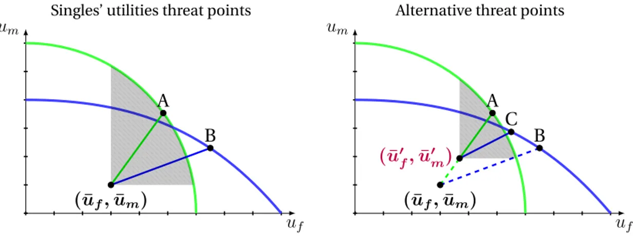
Transferable utilities are nice for they provide a simple example where trans-actions are independent of threat points. For the exact same reason they are not a good choice if our goal is to show how to induce more desirable transactions. So, as a second example consider the general case for which utility is only par-tially transferable. For a givenz = (cf,−nf, cm,−nm), the frontier of the utility
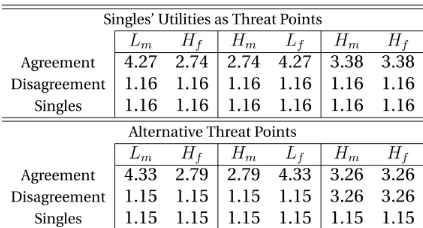
possibility set is no longer a straight line of slope−1. Instead, we represent the utility possibility set for the couple who has chosenzas the convex set bounded by the green curve in Figure 2. Note that this is a conditional utility possibil-ity set, since it is built holding z fixed. The set bounded by the blue curve is the utility possibility set for the same couple it it chose, instead,z′. Point A, in
Singles’ utilities threat points Alternative threat points
uf um
(¯uf,u¯m)
A
B
uf um
(¯uf,u¯m)
A
B C
(¯u′
f,u¯′m)
Figure 2: The blue curve denotes the utility frontier for the same couple for the case in which a false reportη′
6
=ηis made. Point B denotes the utility pair the couple would attain in case of a lie. If the threat points changes from(¯uf,u¯m)to(¯u′f,u¯
′
m)equilibrium choices are not changed,
yet the deviation utility pair changes from B to C.
choice of z, whereas point B denotes the preferred utility pair were the couple to choose transactionsz′. Finally, the green line connecting(¯uf,u¯m)to point A
defines the set of all potential threat points (greater than(¯uf,u¯m)) that induce A
as the optimal choice for this couple, givenz. If the couple were instead choos-ingz′, then the blue line connecting(¯uf,u¯m)to B would represent the analogous
set of threat points that make B the preferred utility pair.
Assume that the couple is just indifferent between A and B. It is therefore just indifferent between transactionszandz′, both assumed to be feasible given the tax schedule in place.14 For concreteness, letzbe the couple’s choice, which we assume to be the one which raises more tax revenues and generate at least as much welfare as judged by the planners’ metric. The planner cannot, in this case, increase this couple’s tax liabilities since this would lead the couple to strictly preferz′.
Now, if the planner were somehow able to induce another threat point along the green curve, e.g., the one denoted(¯u′
f,u¯′m)in Figure2, then Point A remains
the optimal choice for the couple if it choosesz, while point B is no longer the optimal choice for the couple if it choosesz′. It is, in fact, possible to show that A is now strictly better than B; hence,z strictly preferred toz′. Some space for raising more taxes is thus created.
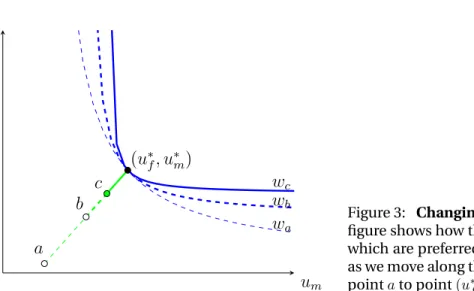
The rationale is, of course, that by moving along the curve we are in fact
14Axiom ’Preference for symmetry’, as defined byZambrano(2016), substitutes for ’symmetry’
a b
c
wa wb wc (u∗
f, u∗m)
um uf
Figure 3: Changing Elasticities. The figure shows how the set of utility pairs which are preferred to(u∗
f, u
∗
m)shrinks
as we move along the curve connecting pointato point(u∗
f, u
∗
m).
reducing the flexibility that the couple has to substitute the utility of one spouse for the other, as shown in Figure 3. We are in practice changing the relevant elasticities.
A welfare improving reform will typically combine elements of the two ex-amples we have offered.
IV Household Choices
Different institutions – tax systems, game forms, etc. – will define the set of transactions that are available to all agents, directly, in the case of tax sched-ules or indirectly for more general mechanisms. To further describe the feasible transactions sets we appeal to the notion of aninstitutional setting, for which we use a generic domination,E.
IV.1 Institutional Settings
An institutional settingE is comprised of setsSi
E, with typical elementsiE,
repre-senting the choice set for a genderisingle agent, andSEc,i, with typical element
sc,iE , the choice set for a genderimarried agent. Completing the description of
E, are functionsζi
E : SEi 7→ Z, mapping choices,siE, into transactions for gender
isingle agents, andζE :SEc,f ×SEc,m 7→ Z × Z for married agents. NowZi
E := ζEi(SEi) ⊂ R2,i =f, m, andZEc := ζE(S
c,f
E ×S
c,m
E ) ⊂ R4 define the
i single agent to realize a transaction z under E it must choose s ∈ Si
E such
that z = ζi
E(s), provided that such s exists. If no such s exists then, z /∈ ZEi.
Similarlyzmay be chosen by a couple ifsf ∈ S c,f
E andsm ∈S c,m
E exist such that z = ζE(sf, sm). Recalling that ZEc is the set of transactions, z ∈ Z2, which are
feasible under the institutional setting E we define for any coupleη, UE(η) :=
S
z′∈Zc
EUz
′(η)⊂R2be the set of all attainable utilities underE.
The next two examples of institutional environments illustrate the defini-tions we are using.
A Simple Tax System — STS A simple tax system is comprised of (possibly) gender based tax schedules for singles and a tax schedule for couples.
We represent a tax schedule by the budget constraint it induces. For a single agent of genderiletTi :R+ 7→Rbe the associated tax schedule. Then, we define
the budget set,Bias
Bi :={z;ψi(c, n) = ψi(z) =c−n−Ti(n)≤0}. (2)
In this case, Si
Ψ = Bi, and ζΨi is the identity mapping. We also define ∂Bi :=
{z ∈Bi;z′ > z ⇒z′ ∈/ B
i}, the frontier ofBi.
A single agent of typeθisolves
max
(c,l)≤(c,1−n),z∈Bi
u(c,l;θi).
We letzi
Ψ(θi)denote the equilibrium transactions and viΨ(θi), the utility
at-tained by a gender isingle agent, i = f, m, under the tax schedule defined in (2).
For couples, letz = (zf, zm). In this case,
Bc
:=z ∈ Z2;ψ(z) = cf +cm−nf −nm−Tc(nf, nm) = 0 . (3)
Analogously to∂Bi, define∂Bc :={z ∈Bc;z′ >z ⇒z′ ∈/Bc}.
The choice setSΨc,iis simplySΨc,f :=Z, whereasζΨis the identity mapping for
ψ(z)≤0, andz= 0, otherwise.
A General Mechanism Agame formormechanism,M, is a collection of mes-sage setsΣs
married agents; outcome functionsgs
i : Σsi → Z for genderisingles, and;
out-come functionsg: Σc
f ×Σ
c
m → Z2, for couples.
That is,
M ≡ {Σs
i,Σci}i=f,m,{g s
i(·)}i=f,m,g
c(·,·). (4)
This definition of a mechanism is mapped into our general notion of an in-stitutional setting by noting that the choice sets are the message spaces,Si
M =
Σs i,S
c,i
M = Σci, i = f, m, whereas the outcome functions areζMi (·) := gis(·), for
singles, andζM(·,·) := gc(·,·), for couples.15
IV.2 Choices in Agreement
Then, for any(¯uf,u¯m)in the interior ofUz(η), let
W(z;η,u¯f,u¯m) :=
max (uf(cf,lf)−u¯f) (um(cm,lm)−u¯m)
s.t. ((cf,lf),(cm,lm))∈Fa(z, η)
. (5)
For each couple η, equation (5) defines a utility function, W : Z2 → R
parametrized by(¯uf,u¯m). W(·;η,u¯f,u¯m), therefore, represents a complete
pre-order in the space of transactions,Z2, for a coupleηwhich threat points areu¯
f
and u¯m. We shall henceforth refer to this ordering as ’household preferences’,
η|u¯f,u¯m, recognizing its dependence on the threat points.
We assume that there is z ∈ Z2 such that for anyη, any((c
f,lf),(cm,lm)) ∈ Fa(z, η), eitheru
f(cf,lf) ≤ uf(ˆcf,ˆlf)for allˆcf,ˆlf ∈ R2+orum(cm,lm) ≤ um(ˆcm,ˆlm)
for allˆcm,ˆlm ∈R2+.
IV.3 The Disagreement Game
A typeη couple maximizes the objective (1), which is only fully specified once threat points are determined. How this determination occurs for each environ-ment is what we discuss now.
15In principle, the outcome function could depend on messages from all agents. Because
Define for anyz∈ Z2,
Φ (zf, zm;η)≡
φf(zf, zm;η) φm(zf, zm;η)
!
= vf
vm
!
(6)
a function which maps transactions z ∈ Z2 into a pair of utilities, (v
f, vm) ∈
R2. This function will play the role of defining the disagreement utilities that
result from any transactions realized by the spouses. We endow Φ(·,·;η) with the following properties: i)for allz, and allη,Φ(z, η)∈U˚z(η), whereU˚z(η)is the
interior ofUz(η);ii)φf(·, zm;η)is increasing inzf for allzm, and;iii)φm(zf,·;η)
is increasing inzmfor allzf.
To make sense of these properties, starting with (ii) and (iii), note that zi
is increased either by making more consumption goods available without an increase in spouse i’s effort, ni or by reducingi’s effort without a reduction in
resources available for consumption of both spouses. We assume that in ei-ther case this increases spouse i’s utility. It may or may not increase his or her spouse’s utility. Because, leisure is not transferable across spouses, a lower ni
can only reduce i’s utility if his or her consumption is substantially reduced. Similarly, provided that a higherci does not lead to a lowerci the assumption is
valid for this case as well.
As for(i), agents act non-cooperatively when they are in disagreement. They will not, in general, be able to reach all points inUz(η). For example, they need
not be able to attain all material gains from cohabitation. We take this into ac-count by assuming that the set of available allocations for spouses in disagree-ment is given by a functionFd(z, η)⊂Fa(z, η).16
For a concrete example of such a function, assume that in disagreement,ci = ci/(cf +cm), i.e., consumption of each spouse is proportional to what each one
contributes to the set of available consumption goods. In this case, provided thatFd(z, η)⊂Fa(z, η),Φhas properties(i)to(iii).
Equilibrium of the Disagreement Game Now to understand how threat points are defined, one must describe howzis determined. Spouseichooses an
ele-16For example, we may consider
Fd(
z, η) :={((cf,lf),(cm,lm)) ; cf+cm≤β[cf+cm] ;lf ≤1−nf/θf;lm≤1−nm/θm},
ment of SEc,i which, along with i’s spouses’ choice, sc,jE is mapped into transac-tions byζEand finally intoi’s utility byφi. Note how the strategy space available
to each spouse depends on the specific institutional arrangements, E, that we are considering. The crucial assumption regarding choices in disagreement is that, in contrast with choices made in agreement, the pair (zf, zm) is selected
non-cooperatively by the couple. That is,zis the (outcome of ) a Nash equilib-rium of a non-cooperative game played by spouses underE.
A key underlying assumption of our approach is that spouses arenot able to commit to a strategy to be used in disagreement.17 We further require spouses
to behave rationally if in disagreement in the sense that each spouse still maxi-mizes his or her own utility.
A final important assumption we make is that no agent can be made worse off than what he or she can attain as a single agent. At any moment and under all institutions that we consider, a spouse may unilaterally call off marriage and attain a utility which is increasing in the utility that someone with her or his productivity attains as a single. One cannot, however, fake one’s marital status. Moreover, a spouses’ decision to become single imposes the same choice on the other spouse.
In most of what follows, to economize on notation, we consider the case in which a single agent and a divorced agent of identical productivities attain the same utility. This is but one possibility for the sensible view that the utility that one may reach upon divorce is an increasing function of the utility that a single agent of the same type can attain.18
Let
χfE(sc,mE , η) := argmax s∈SEc,f
φf (ζE(s, s
c,m
E );η)
define the wife’s reaction function for the game played underE with analogous definition, χm
E(s
c,f
E , η), for the husband. An equilibrium, s∗f = χ f
E(s∗m, η), s∗m = χm
E(s∗f, η), for the disagreement game defines(¯z c,f
E (η),z¯
c,m
E (η)) =ζE(s∗f, s∗m).
Whether a pure strategy equilibrium exists and, when it exists, whether it is unique depends not only on the properties ofΦbut also on those ofE. Thus, for each institution, we make assumptions directly on the game effectively played. Provided an equilibrium does exist,¯zE(η) = (¯zEc,f(η),z¯Ec,m(η))are the transactions
17This rules out many different approaches for determining the threat points — seeMyerson
(1997) for a discussion.
that would be conducted by a coupleηif they were not able to reach an agree-ment under the institutional setting E. We finally use(¯ufE(η),u¯m
E(η))to denote
the threat points that arise underE.
IV.4 Equilibrium Allocations Under
E
Define for each environmentE
ˆ
sE(η,u¯f,u¯m) := argmax sf,sm∈(SEc,f×S
c,m
E )
W(ζE(sf, sm);η,u¯f,u¯m), (7)
theconditional choices by a coupleηwhen threat points are(¯uf,u¯m). We write, ˆ
zE(η,u¯f,u¯m) :=ζE(ˆsE(η,u¯f,u¯m))to denote conditional transactions.
As we have just seen, the institutional setting,E, also determines threat points through the disagreement game it induces. For (¯uf,u¯m) = (¯uf
E(η),u¯mE(η)), i.e.,
when threat points are those that arise in the equilibrium of the disagreement game, we arrive at
sE(η) := argmax
sf,sm∈(Sc,fE ×S
c,m
E )
W(ζE(sf, sm);η,u¯Ef(η),u¯mE(η),
the equilibrium choices for spouses in a coupleηunder institutionsE.19
Equi-librium transactionszE(η), are, thenzE(η) :=ζE(s c,f
E (η), s
c,m
E (η)). We may
there-fore theallocation implemented byE,
n
ziE(θi)θ
i,i=f,m,(zE(η))η
o
, (8)
We let{(vi
E(θi))θi, v
c,i
E (η)
η}i=f,m, represent the associated utility profile.
Aggregate transactions underE are
ZE =
X
i=f,m
ˆ
zi
E(θi)dµis(θi) +
ˆ
zEc,i(η)dµc(η)
An allocation isfeasibleifG(ZE)≤ 0, whereG(·)is the transformation
func-tion that represents the economy’s technology.
19Noting thats
E(η) = (sc,fE (η), s
c,m
E (η)) ′
andzE(η) = (zc,fE (η), z
c,m
E (η)) ′
, we have, for allE and allη,(sc,fE (η), s
c,m
E (η)) = ˆsE(η,u¯fE(η),u¯mE (η)),(z
c,f
E (η), z
c,m
Threat points and commitment Unless otherwise stated we will retain the as-sumption that couples cannot commit to a given behavior in disagreement.
If such commitments were however possible, the set of implementable allo-cations would be significantly restricted.
Proposition 1. For an environmentE, let(vfE(η),vm
E(η))be the pair of equilibrium
utilities that arises for a couple η = (θf, θm)at the maximization (in(sf, sm)) of W(ζE(sf, sm);η, v
f
E(θf), vEm(θm)). Let
VEα:=
n
(uf, um)|∃α∈[0,1]; (uf, um) =α(vfE(η),vmE(η)) + (1−α)(v
f
E(θf), vEm(θm))
o
.
If spouses can commit on disagreement choices, then(¯ufE(η),u¯fE(η))∈Vα
E .
Proof. See AppendixA.1.
Assume that(¯uf,u¯m) in figure2is the utilities that spouses would attain if
they divorced, which we are assuming to be the utilities that single agents with identical productivities attain underE,(vEf(θf), vEm(θm)). In this case,(v
f
E(η),vmE(η))
is point A in the same figure, and the setVα
E is the green line connecting(¯uf,u¯m)
to point A.
V Agreement Randomizations
Thus far we have allowed for non-convex utility possibility sets by replacing
Nash’s (1950) symmetry byZambrano’s (2016) preference for symmetry. An al-ternative approach would be to rule out non-convexity altogether by assuming that households may randomize across different transactions.
To allow for randomization we extend the utility representation to a expected utility representation, and apply the Nash-Bargaining approach over this utility. Let’s consider an example. Suppose that a couple has access to both the fron-tierUz(η)andUz′(η)in Figure4, generated by transactionszandz′, respectively.
Suppose that the planner wants the couple to choose the bundlez.
If the couple cannot randomize, then the relevant Pareto frontier is the en-velope of Uz(η)and Uz′(η). To implementz, the planner only needs to make
sure that there is a point inUz(η)that is better, in the sense of yielding a higher
That is illustrated as point u1 := (uf1, um1 )in Figure4. Pointu2 is the point that
maximizes the Nash product ifz′is chosen, instead.
If spouses are, however, able to randomize, then, in our example, they can attain a better utility pair. This is shown in figure5. The relevant Pareto Frontier is the convex hull ofUz(η)andUz′(η). Notice that the particular randomization
presented in the picture implies that one of the spouses maybe worse in the marriage than his/her disagreement utility.
In this case, to implement z, the planner needs to guarantee no point in
Uz′(η)is above the tangent ofUz(η)and the relevant indifference curve. An
ex-ample where it happens is given on 6, whereas Figure 5provides an example where it does not.
Whether this randomization is a reasonable description about household choices or not crucially depends on how we interpret randomization in this set-ting.
As in Mirrlees (1971) the natural interpretation of our model is that it is a static representation of life-long choices made by individuals. In this sense ran-domization could be seen as an ex-ante commitment to a one of the two allo-cationsuaorub. For this reason, this case is calledRandomization with strong
commitment.
Although possible this seems to contradict the very idea of a collective model. Indeed, one of the underlying justifications for ruling out the unitary model as a valid description of household behavior relies on the inability to commit as explained in?. Hence, if we only assume some form of ’spot’ commitment, then the idea that households decide once and for all to choose an allocation such as
uaorubdoes not seem plausible.20
Alternatively we may be assuming non-stationarity of allocations. Spouses alternate betweenuaandubwith the right frequency. Again, some form of
com-mitment beyond spot comcom-mitment is needed. So, the only interpretation of randomized choices compatible with ’spot commitment’ is literal lottery used in the beginning of each period to decide whether ua or ub will be chosen. If
this is the case, then all utility possibility sets must be convex and threat points will have no baring on incentive compatibility in the convexified range.
A weaker assumption regarding commitment is that couples choose between
20Spouses must commit at least on how to share the consumption goods that are brought
z and z′, and given this choice decide how to share consumption in order to maximize the Nash product. This leads to the following restriction on the plan-ner’s ability to implement the allocations it may desire. Assume that the planner aims at implementingz, in which caseu1 would be chosen. If the couple were
instead to choose z′ then u2 would be chosen instead. Moreover, any lottery
involvingzandz′would lead to a lower value for the household thenu1. In this
case, we would say thatu1was implementable. Otherwise, it would not be.
In other words the couple can only commit to utility pairs that maximize the Nash product for each transaction. Randomization still restricts the set of implementable allocations, but less so than in the case of full commitment. The relevant Pareto Frontier is the convex combination of those. By construction, these points are preferred to the disagreement utility, and are consistent with a new bargaining process after uncertainty is resolved.
To implement z, the planner needs to keep f2 below the tangent to Uz(η)
at f1. We show this on figure 7, notice that there areUz′(η)points above the
tangent.
Up to now we have assumed that disagreement utilities are given. We iden-tified two disagreement effects on the non-random case. Apparently, the dis-agreement can be used on all cases to affect which point onUz(η)is chosen, this
was one of the channels.
The other one was based on changes that kept u1 fixed, but made other
points less desirable, from the couple’s perspective. This channel is ineffec-tive on the Randomization with commitment case, because the disagreement has no effect on the points chosen to randomize. We get the same results with transferable utilities, for a different reason.
This elasticity channel still effective on the Randomization without commit-ment case, as changes on the disagreecommit-ment that don’t changeu1 will affect the
point chosen onUz′(η).
VI Implementable Allocations
um uf
Uz(η)
Uz′(η)
um uf
u1
u2
Figure 4
um uf
u1
E[u]
ua
ub
Figure 5: Randomization between transac-tions z and z′
and commitment to an allo-cation of resources leading to utility pairsua
andubleads to an expected utility pairE[u] :=
um uf
u1
Figure 6: No choices or lotteries involvingz′
lead to a higher Nash product than u1. z is
therefore implementable even if we allow for the strongest possible form of commitment between spouses.
um uf
u1
u2
Figure 7: Pointsu1andu2are the Nash prod-uct maximizing choices for transactions z
and z′
, respectively. Lotteries involving u1
married when in fact single.
VI.1 A Direct Mechanism - DM
In a direct mechanism, Γ, the government asks each agent his or type. Given the economy’s informational structure, we define a single agent’s type as his or her productivity, θi. For couples, a θf woman married to a θm man is said to
have type (θf, θm,a)if the couple is in agreement. If the couple is, instead, in
disagreement the same agent is said to have a type(θf, θm,d). That is, a married
agent’s type, (η, ι) ∈ Θ2 × I,I = {a, d}, is the same as his or her spouses’. Yet,
since gender is public information, a (η, ι)woman can be distinguished from her husband, a(η, ι)man, for all purposes.
For singles, upon a reportθˆi, an outcome functions assigns transactionsz = γs
i(ˆθi). Married agents must also report their type, which, as we have seen, is the
combination of their productivity,θi, their spouses’ productivity,θ−i, fori,−i= f, m, and whether they are in agreement or disagreementι ∈ I := {a,d}. The outcome function γ : (Θ2× I)×(Θ2× I)maps announcements of types into
transactions for both spouses. Hence,Si
Γ = Θ,S
c,i
Γ = Θ2× I,ζΓi(·) :=γis(·), and,
ζΓ(·,·) :=γc(·,·).
Before we formally define incentive-feasibility it is worth providing further details about the disagreement game under the DM. An announcement(ˆη, ι) ∈
Θ2× I by a husband and an announcement(ˆη′, ι′)∈ Θ2× I by his wife induce
transactionsγc(ˆη′, ι′,η, ιˆ ). For couples in disagreement, these transactions map
into a pair of utilities(vf, vm)throughΦ, therefore defining a game in the space
of announcements,Θ2 × I, through the impact of announcements on
transac-tions.
The reaction function forfin a coupleηis, in this case,
χfΓ(ˆηm,ˆιm, η) := argmax
(ˆη,ˆι)∈Θ2
×I
φf γfc(ˆη,ˆι,ηˆm,ˆιm), γmc (ˆη,ˆι,ηˆm,ˆιm);η
, (9)
with analogous definition forχm
Γ(ˆηf,ˆιf, η).
An equilibrium for this game,
(ηf∗, ι∗f, ηm∗, ι∗m) =
χfΓ(ˆη∗m, ι∗m, η), χmΓ(ˆηf∗, ι∗f, η)
defines a pair of threat points,u¯fΓ(η),u¯m
Γ(η)
Note that lies are detected whenever conflicting announcements(η′, ι′, η′′, ι′′)
such that η′ 6= η′′ orι′ 6= ι′′ are made. One of the spouses must be lying when
this happens for they are making two reports over the same information which is common knowledge that they know.
Note that if any spouse chooses to report as single, the couple must split. That is, the condition for using a single agent’s tax schedule is to be single.
We say that a Direct Mechanism - DM - is incentive-feasible if
1. For every single agentθi,
u(γis(θi), θi)≥u(γ s
i(ˆθi), θi)∀θˆi, i=f, m. (10)
2. For every coupleη, and all(ˆη,η, ι,ˆˆ ˆι)∈Θ2× I2,
W(γ(η, a, η, a), η; ¯uf,u¯m)≥W(γ(ˆη, ι,η,ˆˆ ˆι), η; ¯uf,u¯m),, (11)
where,
¯ uf ¯ um
!
= φf(γ(η, d, η, d);η) φm(γ(η, d, η, d);η)
!
(12)
3. For allη,
(η, d)∈arg max
ˆ
η∈Θ2,ι
∈Iφf(γ(ˆη, ι, η, d);η) (13)
and
(η, d)∈arg max
ˆ
η∈Θ2,ι
∈Iφm(γ(η, d,η, ιˆ );η) (14)
4. For anyη= (θf, θm),
vΓc,i(η)≥u(γis(ˆθi), θi)∀θˆi, i=f, m. (15)
5. If the distribution of singles of genderi is given by a measureµi
s and the
distribution of couples is given by a measureµcthen,
G X
i=f,m
ˆ
γs
i(θi)dµis(θi) +
ˆ
γc
i(η, a, η, a)dµc(η)
!
≤0. (16)
The second constraint guarantees that a type η couple in agreement does not misreport its type for threat points which are defined by the pair of utilities that arise when both decide to announce truthfully in case of disagreement. The third constraint is that truth-telling be an equilibrium announcement for spouses in disagreement. The forth constraint imposes the condition that no married agent would rather become single. Constraint five is the feasibility con-straint. Although we do not require feasibility under disagreement, we do im-pose incentive-compatibility.
VI.2 The Revelation Principle
The main result from this Section is that the Revelation Principle is valid in this setting.
Proposition 2. Let
n
zi
M(θi)
θi,i=f,m,(zM(η))η
o
(17)
be an implementable allocation, i.e., an allocation for which there is a mecha-nismMfor which (17) is the equilibrium allocation. There, there exists a Direct
Mechanism - DM - which implements the same allocation.
Proof. See AppendixA.1.
Implementation should be taken here in the weak sense. There is an equi-librium for the direct mechanism that generates the outcome corresponding to the target allocation. We cannot rule out the existence of other equilibria for the direct mechanism generating different outcomes. Nor can we rule out the introduction of equilibrium outcomes which were not equilibria in the original mechanism,M.
As we have noted, an important aspect of implementation in the environ-ment considered here is the ability of manipulating threat points under each institutional setting, an issue we return to next.
VI.3 ’Choosing’ threat points
Under our assumptions, eachE induces a unique(¯ufE(η),u¯m
E(η)) ∈ Φ(Z2, η), for
allocation,({zi
E(θi)}θi,i=f,m,{zE(η)}η), an improvement can only occur through
the replacement ofE by an alternativeE′.
By replacing one institutional setting by another one typically changes not onlyη|u¯f
E,u¯mE but alsoZ c
E. Therefore, even choices may change even if we were
able to holdη|¯uf
E,u¯mE fixed.
To isolate the role of different institutional settings in affecting allocations through their impact on threat points it will be useful to considerE andE′such
that the boundary of the set of available transactions is not altered.
An example of such reform occurs when choice sets and outcome functions change but feasible transactions remain the same, i.e.,SEc,i′ 6=S
c,i
E , butZEc′ =ZEc.
Let ∂Zc
E := {z ∈ ZEc|∄z′ ∈ ZEc such thatz′ >z}, we consider replacing E by E′
such that∂Zc
E′ =∂ZEc.
What is interesting about this latter possibility is that households in agree-ment face exactly the same relevant portions of their budget sets. If zE′(η) 6=
zE(η), for someη, it must be due to changes in the family’s objective. That is,
such reforms only change the ’distribution factors’, e.g., Chiappori and Bour-guignon(1992).
By consideringE′such thatz
E′(η)6=zE(η)we may be describing a complete
reform, or a first step in a full reform to a new institutional settingE′′for which
the set of induced preferences is such that Zc
E′′ 6= ZEc induces a more desirable
allocation.
The first step in the reform does not change the (conditional) utility pos-sibility sets, Uz(η)(η). Note also that, for all η, inequality (11) remains valid if
we hold (¯uf,u¯m) = (¯ufE(η),u¯mE(η))fixed. Of course, this need not imply
incen-tive compatibility: inequality (11) need not be satisfied at the new threat points
(¯u′
f,u¯′m) = (¯u f
E′(η),u¯mE′(η)). It is good that it does not, for it is this very possibility
that motivates an important part of our analysis.21
VII Tax Systems
Following Mirrlees’ (1971) seminal work, the characterization of optimal tax schedules relied on a two steps approach. First, constrained efficient
alloca-21Examples of reforms which respect these restrictions are, in the case of a DM, replacingγ
by someγˆ such thatγ(η, a, η, a) = ˆγ(η, a, η, a)for allη, and for all(η′, ι, η′′, ι′)
,γˆ(η′, ι, η′′, ι′) ≤
tions were first derived using a direct mechanism. Second, budget sets that supported these allocations were derived.
It is our goal in this Section to assess whether tax implementation is with-out loss when couples are non-unitary. In Section VIwe have seen that a DM implements any incentive feasible allocation. We need now ask whether any incentive-feasible allocation can be implemented via tax systems.
We make a distinction between a tax schedule and a tax system, which is how we call a collection of tax schedules. A Simple Tax System - STS, is comprised of a tax schedule for single females, another one for single males and, finally, one for couples. We shall also consider a Dual Tax System - DTS, which, adds to these schedules an alternative schedule for couples which can be chosen upon the manifestation of any one of the spouses. An example of such dual systems is provided by filing options found in countries like the United States.
VII.1 STS and DM: Conditional Equivalence
We have already described an STS in Section II. We shall first show where the difficulties for implementation donot lie by comparing implementable alloca-tions when households’ objective funcalloca-tions are given, i.e., holding threat points fixed.
VII.1.1 Conditional allocations under the STS
The tax schedule of which the STS is comprised defines budget sets for singles of each gender and for couples under which choices are made. In the case of married agents choices may be made in agreement, through the maximization of a functionW(z, η; ¯uf,u¯m), and in disagreement as an equilibrium for the
non-cooperative game played under the tax system.
For any given(¯uf,u¯m)the solution of the household maximization program
under the restriction thatψ(z)≤0, iszˆ(η,u¯f,u¯m)). We shall use the term
condi-tional allocations when we consider changes in the tax system holding(¯uf,u¯m)
fixed.
If a coupleηis in disagreement threat points,(¯ufΨ(η),u¯m
Ψ(η))are determined
the ordering of transactions effectively used by householdηunder the tax sys-tems. The solution to the household problem under this ordering captured by the objectiveW(z, η; ¯ufΨ(η),u¯m
Ψ(η)), finally determines the equilibrium
transac-tionszΨ(η)≡zˆ(η,u¯fΨ(η),u¯mΨ(η))for the tax system.
A STS is feasible ifG(ZΨ)≤0, with
ZΨ :=
X
i=f,m
ˆ
zΨi(θi)dµis(θi) +
ˆ
zΨc,i(η)dµc(η)
.
VII.1.2 Conditional allocations under the DM
A DM defines a set of feasible transactions,{z;∃θi;γi(θi) = z}for genderi,i = f, m, singles and{z;∃(η, i,η, jˆ )∈Θ2× I ×Θ2× I;γc(η, i,η, jˆ ) = z},for couples.
Using (7), we recall that the conditional (on(¯uf,u¯m)) choices by a coupleηunder
the DM are
ˆ
sΓ(η,u¯f,u¯m) := argmax
(η′,ι,η′′,ˆι)∈Θ2×I×Θ2×I
W(γc(η′, ι, η′′,ιˆ), η; ¯uf,u¯m), (18)
The associated transactions arezˆΓ(η,u¯f,u¯m)≡γc(ˆsΓ(η,u¯f,u¯m)).
For each couple η, (¯ufΓ(η),u¯m
Γ(η)) is the pair of threat points which results
from the game described in Section IV.3 under Γ. We say that the allocation is incentive compatible if for every η, ˆsΓ(η,u¯f,u¯m) = (η, a, η, a) for (¯uf,u¯f) = (¯ufΓ(η),u¯m
Γ(η)). Naturally,zΓ(η) = γc(ˆsΓ(η,u¯fΓ(η),u¯mΓ(η)))are the associated
trans-actions.
Our main interest in this Section is to compare the allocations that can be implemented by an STS with those that can be implemented by a DM, when threat points are held fixed. Hence, it will also be important to define conditional (on(¯uf,u¯m)) incentive compatibility assˆΓ(η,u¯f,u¯m) = (η, a, η, a)for a given
ar-bitrary(¯uf,u¯m).
We say that an allocation is implementable by a tax systemψif there is a tax system for which such an allocation is an equilibrium induced byψ. We say that an allocation is implementable by a direct mechanism Γ if there is a truthful equilibrium for the game played under the mechanism, which is mapped into this allocation by the associated outcome function.
Proposition 3. Let
zi
Ψ(θi) θi,i=f,m,{zΨ(η)}η
be the allocation induced by an STS. For every couple, η, let (¯ufΨ(η),u¯m
Ψ(η)) ∈ ◦
UΨ(η) be the equilibrium threat points under the STS. Then, there is a DM, Γ,
such thatzi
Γ(θi) = ziΨ(θi)for allθi,i = f, m.,γc(ˆsΓ(η,u¯fΨ(η),u¯mΨ(η))) = zΨ(η), for
allη.
Proof. Immediate consequence of Proposition2.
Proposition 3 is, of course, a direct consequence of Proposition 2, which states that a direct mechanism can implement any incentive feasible allocation. Still, in Appendix A.1 we offer an alternative direct proof that parallels those found inHammond(1979);Guesnerie(1998) to highlight the fact that it is only in its impact on threat points that the equivalence may fail.
Proposition 4. Let
zi
Γ(θi) θi,i=f,m,{zΓ(η)}η
be the allocation implemented by a DM. For every couple, η, let(¯ufΓ(η),u¯m
Γ(η)) ∈ ◦
UΓ(η)be the equilibrium threat points under the DM. Then, there is a STS,ψ, such
thatzi
Ψ(θi) = zΓi(θi)for allθi,i=f, m.,zˆΨ(η,u¯fΓ(η),u¯mΓ(η)) =zΓ(η), for allη.
Proof. See AppendixA.1.
The logic of both proofs is the same used byHammond(1979) and further explained byGuesnerie(1998). The reason why the result remains true here is because couples have well defined preferences and make choices that respect those preferences,when we hold the threat points fixed.
Hence, we may refine the implementation problem by focusing on the fol-lowing two more specific questions. For an arbitrary STS, is it possible to find a direct mechanism which, at the same time, generates the threat points that arise under the tax system and the household choices that lead to the trans-actions that arise under the STS? Conversely, for any DM, is it possible to find a STS which induces the same threat points that arise as the DM equilibrium threat points while inducing the household transactions that arise under the DM.