Approximate recursive equilibrium with minimal state space

Ensaios Econômicos

Escola de

Pós-Graduação

em Economia

da Fundação

Getulio Vargas

N◦ 737 ISSN 0104-8910

Approximate

Recursive

Equilibrium

with

Minimal State Space

Raad, Rodrigo Jardim

Os artigos publicados são de inteira responsabilidade de seus autores. As

opiniões neles emitidas não exprimem, necessariamente, o ponto de vista da

Fundação Getulio Vargas.

ESCOLA DE PÓS-GRADUAÇÃO EM ECONOMIA Diretor Geral: Rubens Penha Cysne

Vice-Diretor: Aloisio Araujo

Diretor de Ensino: Carlos Eugênio da Costa

Diretor de Pesquisa: Ricardo de Oliveira Cavalcanti Direção de Controle e Planejamento: Humberto Moreira

Vice-Diretor de Graduação: André Arruda Villela & Luis Henrique Bertolino Braido

Rodrigo Jardim, Raad,

Approximate Recursive Equilibrium with Minimal State Space/ Raad, Rodrigo Jardim – Rio de Janeiro : FGV,EPGE, 2013

34p. - (Ensaios Econômicos; 737)

Inclui bibliografia.

Approximate Recursive Equilibrium with

Minimal State Space

Raad, R.

February 17, 2013

Departament of Economics, Federal University of Minas Gerais, UFMG -Brazil.

Abstract

This paper shows existence of approximate recursive equilibrium with minimal state space in an environment of incomplete markets. We prove that the approximate recursive equilibrium implements an approximate sequential equilibrium which is always close to a Magill and Quinzii equilibrium without short sales for arbitrarily small errors. This implies that the competitive equilibrium can be implemented by using forecast statistics with minimal state space provided that agents will reduce errors in their estimates in the long run. We have also de-veloped an alternative algorithm to compute the approximate recur-sive equilibrium with incomplete markets and heterogeneous agents through a procedure of iterating functional equations and without us-ing the first order conditions of optimality.

Keywords: Recursive Equilibrium, Computational Economics, Incom-plete Markets, Approximate Equilibrium.

JEL Classification: D50, D52.

1

Introduction

equilibrium properties in sequential markets under the assumption of com-mon expectations on prices as in Radner (1972). In this model, markets are incomplete in the sense that at every date and for every commodity there will be some future dates and some events at those dates for which it will not be possible to make current contracts for future delivery contingent on those events. In this way, agents make consumption and investment plans contingent on the realizations of possible states of nature, under their own be-liefs, basing the current choices on the optimal planning. The latter depends on how the agents have expectations on prices contingent on the fulfillment of future events representing exogenous uncertainty, i.e., events whose real-izations are independent of agents’ choices. This fact is the essence of the common expectations hypothesis.

There are two natural ways to explain how this equilibrium withcommon expectations can be achieved. The first regards to the high level of coordi-nation among agents who propose to only negotiate at that contingent price level matched in the future. The second takes into account the computing capacity of the agents who use past variables and economic fundamentals to obtain a recursive relation between endogenous variables in two consecutive periods characterized, basically, by recursive transition functions. This set of functions, also called recursive equilibrium,1 _{includes price estimators that}

represent a common recursive price expectation and implements the equi-librium in the sequential markets. Duffie et al. (1994) has a fairly general result showing the existence of such estimators but with a domain containing a large number of variables, which calls into question the assumption that agents can compute the prices accurately. Kubler and Polemarchakis (2004), Spear (1985) and Hellwig (1982) point to a possible generic nonexistence of recursive equilibrium, with few variables in its domain, for the model of overlapping generations. But Kubler and Polemarchakis (2004) show that it is possible to obtain a stream of prices implemented recursively where agents trade goods and assets that makes its optimal utility quite close to that obtained if prices actually confirm their expectations.

The methodology used in the literature to construct a recursive equilib-rium is given in Duffie et al. (1994). Basically, they consider a state space

S containing all pay-off relevant variables and a correspondence G : S →

1

Prob(S), where Prob(S) is the set of Borel probability measures over S. This correspondence is interpreted as the intertemporal consistency, derived from some particular model, embodying exogenous shocks, feasibility con-ditions, and the first order optimality conditions of dynamic programming problems of the agents. A measurable subset S′ _{⊂ S is said to be}

self-justified if G(s)∩Prob(S′_{)6=∅ for all s∈S}′_{. Under regular assumptions on}

G, DGMM show that, if there exists a non-empty compact self-justified set

S′ _{⊂ S, then G admits a measurable selection and, using the Skorokhod’s}

Theorem, they find a stationary function g defined2 _{in S}′ _{relating two}

con-secutive realizations of the equilibrium stochastic process. The approximate recursive equilibrium defined in Kubler and Polemarchakis (2004) is a func-tion whose domain contains few variables and that approximates the selector

g, but might be very far from exact equilibrium as presented in Kubler and Schmedders (2005). The latter paper exhibits an example that illustrates this fact, with zero intertemporal discount rate and the estimation error con-sisting only in the first order conditions in the optimization problem of the agents. Moreover, they develop theoretical foundations for an error analy-sis of approximate equilibrium providing sufficient conditions to ensure that approximate equilibrium are close to exact equilibrium. Kubler (2011) also examines the relationship between exact and approximate recursive equilib-rium for economies whose fundamentals are semi-algebraic, that is, instan-taneous utility and production functions can be described by finitely many polynomials.

In this paper, we show the possibility of a sequential equilibrium be even-tually achieved (and computed) with common expectations as in Radner (1972) or Magill and Quinzii (1996), even without assuming a high level of coordination among agents. As in Duffie et al. (1994) and in Kubler and Polemarchakis (2004), we construct estimators that implement the prices and allocations of consumption and asset shares so that agents maximize their expected utility but with arbitrarily small errors in the market clearing conditions. However, these estimators are constructed through a selection of a correspondence defined without using the first order conditions of optimal-ity and so that one can always implement a sequential equilibrium arbitrary closed to an exact equilibrium. We do not need to assume further conditions

2

such as in Kubler (2011) and, contrary to the definition of approximate equi-librium given in Kubler and Polemarchakis (2004), the optimality choices are exact in our approach, avoiding the criticism of Kubler and Schmedders (2005). We assume that the demand for current assets can not expand arbi-trarily as a function of asset endowments in the previous period and current prices, constructing an example with one good and one asset clarifying this assumption. Furthermore, we show that these estimators are continuous and contains a domain with the smallest possible number of variables, also called minimal state space.3 _{Contrary to Duffie et al. (1994), we use a constructive}

argument explaining how, in sequential markets, the equilibrium can be im-plemented recursively by the transition functions by showing explicitly the consecutive relations among endogenous variables. Finally, we show an alter-native way to compute an equilibrium, with heterogeneous agents obtaining the estimators, without using the first order conditions, through a procedure of iterating functional equations. Computing the value function and the de-mand through its argmax, we obtain approximations whose errors do not propagate over time as pointed out by Kubler and Schmedders (2005) about the method of Scarfh (1967) which approximates the first order conditions. Indeed, the value function is the optimal value among the current choices and all feasible plans over all future periods and the errors are generated only through the value function.

2

The model

2.1

Definitions

Suppose that there exist a finite set of types denoted by I = {1, ..., I} and such that each typei∈ I has a continuum of agents trading in a competitive environment. Time is indexed by t in the set N _{= {1,2, ...} for current}

periods and r ∈ N_{∪ {0} for future periods. In this model, the uncertainty}

is exogenous, in the sense of being independent of agents’ actions. Each agent knows the whole set of possible exogenous variables, also called states of the nature, and trade contingent claims. Let Z be a finite set containing all states of the nature and Z _{its σ-algebra. Denote by (Zt,}Z_{t) a copy of}

3_{This set contains the portfolio asset endowment of previous period and the current}

(Z,Z_{) for all t ∈} N_{. Exogenous uncertainty is described by the streams}

zt _{= (z}

1, ..., zt)∈Z1× · · · ×Zt=Zt for all t∈N, that is, the set of nodes of

the event tree is given by S_t∈NZ

t_.

There are a finite set J = {1, ..., J} of goods and a finite set H =

{1, ..., H} of long lived real assets in net supply equal to one and with

divi-dends characterized by measurable bounded functions ˆd:Z →RJ H_{++ in units}

of goods. The matrix element ˆdjh(z) of ˆd(z) represents the amount of goodj

paid by one unit of asset h in the state of the nature z. Denote by Θi _⊂RH

+

for all i ∈ I the convex set where asset choices are defined and Ci _{⊂ R}J

+

the convex set where agent i’s consumption is chosen. Observe that we are not allowing for short-sales. Define the symbol without upper index as the Cartesian product. For instance, write C=Q_i∈ICi_.

Denote by Q = {(qc_{, q}a_{) ∈ R}J

+ × RH+ :

P

j∈J q c j +

P

h∈Hq a

h = 1} the

set where the prices are defined and write Q◦ _{= Q∩ R}J+H

++ . The symbol

q = (qc_{, q}a_{) ∈ Q stands for the consumption and asset prices in units of}

the num´eraire respectively. We write qc_dˆ

h(z) :=P_j∈J qcjdˆjh(z) ∈R+ as the

amount of the num´eraire paid by one unit of asset h and write qc_dˆ_(z)θi _:=

P

h∈Hq c_dˆ

h(z)θhi ∈R+ as the amount of the num´eraire paid by the portfolio

θi _∈RH

+. In addition, we define ˆd(z)θi =

P

h∈Hdˆh(z)θ i

h ∈ RJ for all θi ∈Θi

as the amount of goods 1, ..., J resulting from the ownership of the portfolio

θi_.

Write Θ = {θ¯ ∈ Θ : P_i∈Iθ¯i

h = 1 for allh ∈ H}. An element ¯θ ∈ Θ

stands for the mean aggregate asset choice of the agents.

LetS = Θ×Z be the space of state variables endowed with the product topology with a typical element denoted by s = (¯θ, z). Write S _{the Borel}

subsets of S and (St,St) a copy of (S,S) for all t∈N. The set St contains

the variables on which the beliefs will be defined. Write the set of all con-tinuous4 _{functions ˆq : S → Q by Qb and the set of all continuous functions}

ˆ

q :S→Q◦ _{by Q}b◦_.

Every Cartesian product of topological spaces is endowed with the prod-uct topology and any set of bounded continuous functions is endowed with the topology induced by the sup norm. The norm || · ||inRn _{considered here}

is the max norm, that is, ||x||= max{|x1|, ...,|xn|}.

The instantaneous utility is a bounded real valued functionui _:RJ

+ →R+

strictly concave and strictly increasing for alli∈ Iwhere the symbol∂jui(ci)

stands for the partial derivative of ui _{with respect to the j-th coordinate}

evaluated at the point ci_.

Each agenti has a measurable endowment ei _{:Z →R}J

+ of goods 1, ..., J.

2.2

Agents’ features

Agents’ beliefs at every fixed daterare characterized by the continuous5 _map

µi

r : Z → Prob(Zr) for r ∈ N, anticipating future exogenous states of the

nature given the realization of the current state of naturez. We suppose that these beliefs arepredictivein the context of Blackwell and Dubins (1962) with continuous probability transition rules λi _{: Z → Prob(Z) where Prob(Z) is}

endowed with the weak topology. More precisely, the measure µi

r satisfies6

for a rectangle A1×...×Ar:

µi

r(z)(A1, ..., Ar) =

Z

A1

· · · Z

Ar

λi_(z

r−1, dzr)· · ·λi(z, dz1).

Remark 2.3. Consider a stochastic process{z˜t}t∈N defined on some

underly-ing probability space and with range in the probability space Z. A proba-bility transition rule on the period t can be regarded as a generalization of the notion of conditional probability of ˜zt+1 given ˜zt with respect to agents’

subjective probability within the framework of Savage (1954).

We follow the approach of contingent choices as given in Radner (1972). As the model described here does not assume market completeness, then agents may not be unwilling to make contracts that implement some future path of consumption as in the Arrow-Debreu equilibrium. Since agents do not perfectly anticipate the future states of nature, which are given exogenously, rationality leads them to make plans for the future at each current period contingent to all possible future trajectories of the states of nature. Therefore we have the definition below.

Definition 2.4. The agent i’s plan at some period is defined as the current period choice (ci

0,θi0)∈Ci×Θi and the streams{cir}r∈N and{θ_ri}_r∈N of mea-surable functions ci_r :Zr _{→ C}i _{and θ}i

r : Zr →Θi for all r ∈N representing

future plans.

5_{The set Prob(Z}r_{) is endowed with the weak topology.}

6_{See Stokey et al. (1989) chapters 8 and 9 for details about the topology of Prob(Z), the}

Remark 2.5. In each current period, the quantity ci

r(zr) can be interpreted

as the value planned for consumption r periods ahead if zr _{is the partial}

history of prices actually observed at these periods. The asset plan {θj r}r∈N

has analogous interpretation.

We assume that the agents choose a feasible plan of consumption and in-vestment that maximizes the expected utility, under their own beliefs, among all other feasible plans. The next definitions characterize the feasibility of a plan and how agents calculate its expected value.

Definition 2.6. Let Bi _{: Θ}i_{×Z ×Q→C}i_×Θi _{be defined as}

Bi(θ_-i, z, q) = {(ci, θi)∈Ci×Θi :qcci+qaθi ≤(qa+qcdˆ(z))θ_-i +qcei(z)}.

Let q = {qr : Zr → Q}r≥0 be a stream of contingent prices for a given

q0 ∈ Q. A plan (ci,θi), for an agent i ∈ I, is feasible from (θ-i, z,q) if

(ci

0,θ0i)∈Bi(θi-, z,q0) and

(ci_r(zr_),θi

r(zr))∈Bi(θir−1(zr−1), zr,qr(zr)) for all zr ∈Zr

and for all r ∈N_.

Denote by Fi_(θi

-, z,q) the set of all feasible plans from (θi-, z,q).

Now we can define the expected utility.

Definition 2.7. Let Ci _{be the set of all sequence of measurable functions}

{ci

r :Zr → Ci}r≥0 with ci0 ∈ Ci for r ∈N. We define the agent i’s expected

utility Ui :Ci×Z →R _{for consuming c}i _{given the state z ∈Z:}

Ui(ci, z) =ui_(ci

0) +

X

r∈N

Z

Zr

βr_ui_(ci

r(z r_))µi

r(z, dz

r_).

Definition 2.8. Define the value function vˆi _{: Θ}i_{×Z →R by:}

ˆ

vi_(θi

-, z,q) = sup{Ui(ci, z) : (ci,θi)∈Fi(θi-, z,q)}. (1)

The following definition characterizes the agents’ demand. Although this demand is independent of time, it yields the current choice at period t given some past and current observed variables for each t ∈ N_{. This approach}

Definition 2.9. We define the agent i’s demand for good and asset by:7

δi_(θi

-, z,q) = argmax{Ui(ci, z) : (ci,θi)∈Fi(θi-, z,q)}.

The result below can be found in Raad (2012) using that the intertemporal budget correspondence is continuous in the product topology and the Berge Maximum Theorem.

Proposition 2.10. The value function vˆi _{is continuous on the set}

{(θ_-i, z,q) : (q₀a+q₀cdˆ(z))θi_-+q₀cei(z)>0}.

The lemma below ensures that the demand becomes arbitrarily large for arbitrarily low prices.

Lemma 2.11. For each compact Ce ×Θe ⊂ Int(C ×Θ) there exists γ > 0

such that if (¯θ, z,c,θ,q) satisfies(ci,θi)∈δi_(¯θi_{, z,q), (c}i

0,θi0)∈Cei×Θei and

(ci

r(zr),θir(zr))∈Cei×Θei for all zr ∈Zr and all i∈ I then q0 ≥γ.

Proof: See Lemma 7.10 in the Appendix. ✷

3

Recursive and sequential equilibrium

Roughly speaking, we can say that a recursive equilibrium is a function relating the variables of equilibrium between two consecutive periods. Duffie et al. (1994) shows the existence of recursive equilibrium in models with heterogeneous agents and state space containing all pay-off relevant variables. Kubler and Polemarchakis (2004) argues that a recursive equilibrium having a reduced state8 _{space may not exist in a model of overlapping generations}

and heterogeneous agents. Furthermore, Kubler and Schmedders (2002) also shows an example of the non existence of recursive equilibrium for the case of a minimal space state pointing to the study of approximate recursive equilibrium as a solution to the problem of coordination and the calculation of the sequential equilibrium numerically. This is our goal hereafter.

The next definition specifies the sequential equilibrium of the economy, also called competitive equilibrium.

7_{This correspondence can be empty whenC}i_×Θi _{is not compact.}

Definition 3.1. Consider the following measurable

1. q :={qr :Zr →Q◦}r≥0 contingent prices;

2. c:={cr :Zr →C}r≥0 contingent consumption allocation;

3. θ :={θr :Zr →Θ}r≥0 contingent portfolio allocation.

Let θ¯be a previous portfolio distribution and z a current state of the nature in a period t. Then these allocations and prices constitute an equilibrium for

E in a period t if satisfy for all zr _∈Zr_:

1. optimality: (ci,θi)∈δi_(¯θi_{, z,q);}

2. asset markets clearing:9 P

i∈Iθ i

r(zr) =1∈RH;

3. good markets clearing: P_i∈Ici_r(zr_{) = ˆd(z}

r)·1+Pi∈Ie i_(z

r).

The concept approximate sequential equilibrium is similar to that given in Kubler and Polemarchakis (2004), consisting of a set of allocations of consumption and portfolio and a stream of prices balancing all markets ap-proximately. However, contrary to Kubler and Polemarchakis (2004), here agents maximize the expected utility achieving the exact optimal benefit at that level of prices.

Definition 3.2. Given ǫ >0, consider the following measurable

1. q :={qr :Zr →Q◦}r≥0 contingent prices;

2. c:={cr :Zr →C}r≥0 contingent consumption allocation;

3. θ :={θr :Zr →Θ}r≥0 contingent portfolio allocation.

Let θ¯be a previous portfolio distribution and z a current state of the nature. Then these allocations and prices constitute anǫ-approximate sequential equi-librium for E in some period if satisfy for all zr _∈Zr_:

1. (ci,θi)∈δi_(θi

-, z,q); 2. ||P_i∈Iθ_ri(zr_{)−1|| ≤ǫ;}

3. ||P_i∈Ici_r(zr_)−ei_(z

r)−dˆ(zr)·1|| ≤ǫ.

We introduce now the concept of approximaterecursive equilibrium and show in the appendix that it implements the sequential equilibrium of the economy. The recursive demand will be constructed using the value function. The latter is defined as the optimal value among all feasible plans, given the income and current portfolio endowments and, in addition, the transitions of the endogenous variables such as prices and asset distribution.

WriteΘ the space of all continuous functions ˆb θ :S →Θ representing the transition of asset distributions. A well known result states that for each

i ∈ I there exists a bounded value function vi _{: Θ}i _{×S ×Q}b◦ _{× Θ}b _{→ R}

satisfying the Bellman Equation:

vi_(θi

-, s,q,ˆ θˆ) = sup

u(ci_{) +β}

Z

Z

vi_(θi_{,(ˆθ(s), z}′_{),q,ˆ θ}ˆ_)λi_{(z, dz}′₎

(2)

over all10 _(ci_{, θ}i_{) ∈ B}i_(θi

-, z,qˆ(s)). Indeed, write V the space of all bounded value functions vi _{: Θ}i_×S×Qb◦_×Θb _{→R endowed with the sup norm and}

consider the operator Ti _{:V→V, defined by}

Ti(vi)(θ_-i, s,q,ˆ θˆ) = sup

u(ci) +β

Z

Z

vi(θi,(ˆθ(s), z′),q,ˆ θˆ)λi(z, dz′)

(3)

over all (ci_{, θ}i_{) ∈ B}i_(θi

-, z,qˆ(s)). Clearly, T satisfies Blackwell’s sufficient conditions for a contraction and hence has a fixed point. See Stokey et al. (1989) for further details.

Definition 3.3. Define the agent i’s consumption and portfolio policy cor-respondence x˜i _{: Θ}i_×S×Qb◦_×Θb _→Ci_×Θi _as

˜

xi_(θi

-, s,q,ˆ θˆ) = argmax

u(ci_{) +β}

Z

Z

vi_(θi_{,(ˆθ(s), z}′_{),q,ˆ θ}ˆ_)λi_{(z, dz}′₎

over all (ci_{, θ}i_)∈Bi_(θi

-, z,qˆ(s));

Remark 3.4. Notice that the policy correspondence satisfy

˜

xi_(θi

-, s,q,ˆ θˆ)⊂Bi(θ-i, z,qˆ(s)) for all (θi-, s,q,ˆ θˆ)∈Θi×S×Qb◦×Θb. (4) Observe also that when ˜xi _{is a function, then it can be written as ˜x}i _{= (˜c}i_,θ˜i₎

for continuous functions ˜ci _{: Θ}i_×S×Qb◦_{×Θb →C}i_{and ˜θ}i _{: Θ}i_×S×Qb◦_{×Θb →}

Θi_{. The lemma below and the strict concavity of u}i _{assure that we can}

assume, without loss of generality, that ˜xi _{is actually a function. To show}

this, it suffices to note that the optimal portfolio choices are unique within the portfolio reallocations that result in the same pay off.

Lemma 3.5. Suppose that Ci _×Θi _{= R}J+H_{. Then the correspondence x˜}i

has a continuous selector.

Proof: See Lemma 7.9 in the Appendix. ✷

Definition 3.6. We say that the economy has an ǫ-approximate recursive equilibrium if there exist continuous functions ˆci _{: S → C}i_{, θ}ˆi _{: S → Θ}i _for

i∈ I and qˆ:S →Q◦ _{satisfying for each s = (¯θ, z)∈S}

1. (ˆci_(s),θˆi_(s))∈x˜i_(¯θi_{, s,q,ˆ θ}ˆ_{) for all i∈ I and s∈S;}

2. ||P_i∈Icˆi_(s)−ei_(z)−dˆ_{(z)·1|| ≤ǫ;}

3. ||P_i∈Iθˆi_{(s)−1|| ≤ǫ.}

The next definition provides more details of how the recursive functions can implement an ǫ-approximate sequential equilibrium.

Definition 3.7. We say that the functions ˆc : S → C, θˆ : S → Θ and

ˆ

q :S→Q generate the process (cr,θr,qr)r≥0 starting from θ¯∈Θ and z ∈Z

if for all zr _∈Zr

q₀ = ˆq(¯θ, z), θi₀ = ˆθi(¯θ, z), ci₀ = ˆθi(¯θ, z)

and recursively for r∈N

ci_r(zr_{) = ˆc}i_(θ

r−1(zr−1), zr) θir(zr) = ˆθi(θr−1(zr−1), zr) (5)

for i∈ I and

qr(zr) = ˆq(θr−1(zr−1), zr). (6)

The next result assures that the recursive equilibrium can actually be used to construct the sequential equilibrium.

Theorem 3.8. If (ˆc,θ,ˆ qˆ) is an ǫ-approximate recursive equilibrium then its implemented process (c,θ,q) starting from (¯θ, z) ∈ S is an ǫ-approximate sequential equilibrium of the economy with initial asset holdings θ¯∈ Θ and initial state of the nature z.

4

Existence and Convergence Results

4.1

Existence of an approximate recursive equilibrium

In this section we will demonstrate the existence of approximate recursive equilibrium with state space S= Θ×Z. For simplicity, we will make a slight change in notation.

Notation 4.2. Write L ={1,2, ..., L} for L =H+J ≥2 and for each γ >0 the set Qγ = Q ∩[γ,1]L ⊂ RL++. Consider Xi = Ci ×Θi ⊂ RL+ convex

with 0 ∈ X and Q′ _{= (0,1]}L _{the set of generalized prices.}11 _{Define X}bi _as

the set of all bounded continuous functions ˆxi _{: S → X}i _{and Q}b′ _{the set}

of all bounded continuous functions ˆq : S → Q′ _{both endowed with the}

topology induced by the sup metric. Recall that Qb is the set of all bounded continuous normalized prices ˆq:S →Q. ConsiderVi _:Xi_×S×Xb_×Qb′ _→Ra

bounded continuous function such thatVi_{(·, s,x,ˆ qˆ) is concave and increasing}

for all (s,x,ˆ qˆ) ∈ S × Xb × Qb′ _{and all i ∈ I. Moreover we suppose that}

Vi_(xi_{, s,x,ˆ ·) is homogenenous of degree zero for all (x}i_{, s,xˆ)∈X}i_×S×Xb.

Write ˆwi _{: S → W}i _{⊂ R}J+H _{as the agent i’s contingent endowments with}

Wi _{compact convex. Recall that we consider || · || as the max norm in R}L_,

that is, ||x||= max{|x1|, ...,|xn|}.

The next definitions will be useful in the main result of this section.

Definition 4.3. Define ˇvi _:S×Xb_×Qb′ _{→R by}

ˇ

vi_{(s,x,ˆ qˆ) = supV}i_(xi_{, s,x,ˆ qˆ) :x}i _∈Xi _{and qˆ(s)x}i _{≤qˆ(s) ˆw}i_{(s) (7)}

and xˇi _:S×Xb _×Qb′ _{→R by}

ˇ

xi_{(s,x,ˆ qˆ) = argmaxV}i_(xi_{, s,x,ˆ qˆ) :x}i _∈Xi _{and qˆ(s)x}i _{≤qˆ(s) ˆw}i_{(s) . (8)}

Remark 4.4. Note that ˇvi_{(s,x,ˆ ·) and ˇx}i_{(s,x,ˆ ·) are homogeneous of degree}

zero for all (s,xˆ)∈S×Xb.

We will define below the Lipschitz property. This property is related to the level of oscillation of a function. For differentiable functions this means that the function must have bounded derivative.

11

Definition 4.5. A functionf :Y ⊂Rn_→Rm _{isM-Lipschitz for M ∈R}

++

if ||f(y)−f(y′_{)|| ≤M||y−y}′_{|| for all y, y}′ _{∈Y.When M ∈R}m

++ then we say

that f = (f1, ..., fm) is M-Lipschitz if fk :Y ⊂ Rn →R is Mk-Lipschitz for

k = 1, ..., m. We write Lp(M) the space of all M-Lipschitz functions.

Remark 4.6. Notice that a function f : Y ⊂ Rn _→ Rm _{∈ Lp(M) for M ∈} Rm_{++ then f ∈Lp(||M||).}

The hypothesis below precludes the possibility of a situation similar to that described by Hellwig (1982) for the case of approximate recursive equi-librium. It states that small variations in asset endowments can not produce arbitrary large fluctuations in asset demand considering that prices fluctuate in a controlled magnitude. Hellwig (1982) points to the impossibility of ex-istence of a stationary function that relates the equilibrium variables, with rational expectations, between two arbitrary consecutive periods providing and example with demand having arbitrary large fluctuation. We give an example below which clarifies this assumption.

Assumption 4.7. Suppose thatXi _=RL_{. Assume that the correspondence}

ˇ

xi _{has a continuous selector ˇδ}i _:S×Xb _×Qb′ _→Xi_{. In addition the function}

ˆ

δi _:Xb _×Qb′ _→Xbi _{defined by}

ˆ

δi(ˆx,qˆ)(s) = ˇδi(s,x,ˆ qˆ) for alls = (¯θ, z)∈S and all i∈ I (9)

satisfies the following property: there exists Mq, Mx > 0 such that if ˆq ∈

Lp(Mq) and ˆx∈Lp(Mx) then ˆδi(ˆx,qˆ)∈Lp(Mx).

Example 4.8. Consider a model with one good and one asset and agents with instantaneous utility function defined by ui_{(·) ≡ ln(·) for i = 1,2.}

Suppose that there is not exogenous uncertainty, that is, Z ={1}andS= Θ. Dividends are given by dˆand there is not good endowments. We must impose that Ci _⊂R

++ and Θi ⊂R++ because ui is defined only for R++. The value

function satisfies

vi_(θi

-,θ,¯ q,ˆ θˆ) = sup

n

ui_(ci_{) +βv}i_(θi_{,θˆ(¯θ),q,ˆ θˆ) : (c}i_{, θ}i_)∈Bi_(θi

-,qˆ(s))

o

(10)

and is strictly concave12 _{on θ}i

-. Since ui is strictly concave on ci then, in this example, the policy correspondence x˜i _{given in definition 3.3 is actually}

function. Let θ˜i _{: Θ}i_×Θ×Qb′ _×Θb _→Θi _{and c˜}i _{: Θ}i_×Θ×Qb′_×Θb _→Ci _be

the policy functions as in Remark 3.4. Lemma 7.7 in appendix assures that

(˜ci_,θ˜i_{) is nonempty and satisfies (˜c}i_,θ˜i_{)>0. Observe that:}

˜

ci_(θi

-,θ,¯ q,ˆ θˆ) =−pˆ(¯θ)˜θi(θ-i,θ,¯ q,ˆ θˆ) + (ˆp(¯θ) + ˆd)θi- (11)

where we write pˆ≡qˆa_/qˆc_{. Fix (θ}i

-,θ,¯ q,ˆ θˆ)∈Θi×Θ×Qb′ ×Θb with θi- >0. We claim that

˜

θi(θi_-,θ,¯ q,ˆ θˆ) = β(ˆp(¯θ) + ˆd)θ

i

-ˆ

p(¯θ) and ˜c

i

(θi_-,θ,¯ q,ˆ θˆ) = (1−β)(ˆp(¯θ) + ˆd)θ_-i.

Indeed, using that u′_{(c) = 1/c and applying the Benveniste and Scheinkman}

Theorem13 _{in Benveniste and Scheinkman (1979) we conclude that}

∂1vi(θ-i,θ,¯ q,ˆ θˆ) = ∂ui(˜ci(θi-,θ,¯ q,ˆ θˆ))(ˆp(¯θ) + ˆd)

= (ˆp(¯θ) + ˆd)/((1−β)(ˆp(¯θ) + ˆd)θi

-)

= 1/((1−β)θi_-)

and hence

∂1vi(˜θi(θi_-,θ,¯ q,ˆ θˆ),θˆ(¯θ),q,ˆ θˆ) = 1/((1−β)˜θi(θi_-,θ,¯ q,ˆ θˆ))

= ˆp(¯θ)/((1−β)β(ˆp(¯θ) + ˆd)θi_-)

for all (θi

-,θ,¯ q,ˆ θˆ)∈Θi×Θ×Qb′×Θb. Therefore

ˆ

p(θ)∂ui(˜ci(θi_-,θ,¯ q,ˆ θˆ)) = ˆp(θ)/((1−β)(ˆp(¯θ) + ˆd)θ_-i) =βpˆ(θ)/((1−β)β(ˆp(¯θ) + ˆd)θi

-)

=β∂1vi(˜θi(θ_-i,θ,¯ q,ˆ θˆ),θˆ(¯θ),q,ˆ θˆ)

which implies that θ˜i _{satisfies the first order condition on θ}i _{of the Bellman}

Equation (10) replacing ci _{by −pˆ(¯θ)θ}i_{+ (ˆp(¯θ) + ˆd)θ}i

-. The strict concavity of

ui _{and of v}i _{on the first coordinate is sufficient to conclude our assertion.}

Consider P ⊂ R_{++ closed.}14 _{Clearly, the function g}i _{: Θ ×P →} R₊

defined by gi_(θi

-, p) = (1 +d/p)θi- satisfies gi ∈ Lp(M′) for some constant

13

See also Stokey et al. (1989) for more details about this theorem.

14

M′_{, since it has bounded derivative. Therefore, it is possible to find M} x =

(Mc_{, M}a_{) and M}

q such that the function

¯

θ7→θ˜i_(¯θi_{,θ,¯ q,ˆ θˆ) = βg}i_(¯θi_,qˆa_(¯θ)/qˆc_{(¯θ))∈Lp(M}a₎

and that c˜i _∈Lp(Mc_{) by using (11) if qˆ∈Lp(M}

q) and θˆ∈Lp(Ma)15

Finally, the following lemmas are useful in the proof of the main result of this section. Its result will be used to construct an operator whose fixed point is the recursive equilibrium.

Lemma 4.9. Consider Y ⊂Rn _{and M, N ∈}R_{++. Suppose that f : Y →Y}

is such that f ∈ Lp(M) and g : Y → Y ∈ Lp(N). Then f ◦g ∈ Lp(M N),

f +g ∈Lp(M +N).

Proof: See Lemma 7.4 in the Appendix. ✷

Lemma 4.10. Consider E ⊂RL_{, γ <1/L and let π}

γ :E →R be defined by

πγ(ξ) = max{qξ :q ∈Qγ}. Then given ǫ >0 the correspondence

ξ→ {q ∈Qγ :πγ(ξ)−qξ ≤ǫ}

has a selector ∆ : E →Qγ with ∆∈Lp(4L/ǫ).

Proof: See Lemma 7.6 in the appendix. ✷

The next assumption holds for the model on which Vi _{is defined using}

the value function vi _{as clarified by Theorem 4.13.}

Assumption 4.11. For each compact Xe ⊂ IntX there exists γ > 0 such that if ˆq ∈ Qb satisfies ˆδi_{(ˆx,qˆ)(S) ⊂ X}ei _{for all i ∈ I and some ˆx ∈ X}b_{, then}

ˆ

ql(s)≥γ for all l∈L and all s∈S.

Theorem 4.12. Suppose Assumptions 4.7 and 4.11 and consider that ˆδi

defined in Assumption 4.7 for i ∈ I. Then for each fixed ǫ > 0 there exist continuous functions xˆi _{: S → R}L

+ for all i ∈ I and qˆ: S → Q◦ such that

ˆ

xi _∈δˆi_{(ˆx,qˆ) for all i ∈ I and ||}P

i∈I(ˆxi(s)−wˆi(s))|| ≤ǫ where || · || is the

max norm and xˆ= (ˆxi₎ i∈I.

Proof: We can suppose without loss of generality that16 _{ǫ≤1. DefineX}i

a compact convex cube containing the compact set17

e

Xi _{= Pr}

i

n

x∈RLI_{+ :}X

i∈I

xi _≤X

i∈I

max{wˆi_{(s) :s∈S}+1}o ₍₁₂₎

in its interior relative to RL_{+. Write X =} Q

i∈IX

i _{and let ˆδ}i _the

corre-spondence given in (9). We can assume that the range of ˆδi _{is contained}

in Xi_{. Indeed, if not, choose m}i _{= supX}i _{∈ R}L

++ and define ¯δi(ˆx,qˆ)(s) =

min{mi_{, δ}i_{(ˆx,qˆ)(s)} ∈ X}i _{for all s ∈ S. Clearly, x}i_{(s) = ¯δ}i_{(ˆx,qˆ) implies}

ˆ

q(s)ˆx(s)≤qˆ(s) ˆwi_{(s) and ¯δ}i_{(ˆx,qˆ)∈Lp(M}

x) if ˆq ∈Lp(Mq) and ˆx ∈Lp(Mx).

Thus ¯δi _{keep all necessary properties to the remainder of the proof since, in}

the approximate equilibrium (ˆx,qˆ), we must have ¯δi_{(ˆx,qˆ) = δ}i_{(ˆx,qˆ) ∈ X}bi

for all i ∈ I by (12). Let ˆξ : X ×W → RL _{be the excess of demand}

function defined by ˆξ(x, w) = P_i∈I(xi _{− w}i_{). Since ˆξ is continuous and}

X ×W is compact, there exists M′ _{> 0 such that ||ξ}ˆ_{(x, w)|| ≤ M}′ _{for all}

(x, w)∈X×W. Consider γ′ _{as in Lemma 4.11 with respect to the compact}

set given in (12) and write N = max{16IL(Mx +Mw)/(γ′ǫ),1}. Choose

γ <min{ǫγ′_/(2M′_{),1/4, γ}′_{}/L and Q}′

γ =Q′ ∩[γ,1]L. Define

b

Q′

γ ={qˆ∈Qb

′_{∩Lp(N) : ˆq(S)⊂Q}′

γ} and Xb

′ _{=Xb ∩Lp(M} x).

Ascoli’s Theorem in Royden (1963) and the compactness ofQ′

γ andX assure

thatQb′

γ and Xb′ are compact. Define the function ˆ∆ : Xb′ →Qb′γ as ˆ∆(ˆx)(s) =

∆( ˆξ(ˆx(s),wˆ(s))) for all s ∈ S where ∆ : Z → Qγ ⊂ Q′γ is given in Lemma

4.10 for the errorǫγ′_{/4 and the lower boundγon prices. Lemmas 4.9 and 4.10}

also guarantees that ˆ∆(ˆx) ∈ Qb′

γ since ˆw ∈ Lp(Mw) implies that Pi∈Ixˆi −

ˆ

wi _∈Lp(I(M

x+Mw)).

WriteN′ _{= min{M}

q/N,1}. LetT :Xb′×Qb′γ →Xb′×Qb′γbe the continuous

convex valued correspondence (function) defined by:

T(ˆx,qˆ) = Y

i∈I

ˆ

δi(ˆx, N′qˆ)×∆(ˆˆ x).

16_{In the case ofǫ >1 remake all arguments replacing ǫby 1.}

17_{A cube in R}L _{is a product of a compact interval contained inR. Moreover, for a set}

Xi_⊂RL

+, write supXi = (supXli)l≤L ∈RL+ where Xli ⊂R+ is the projection ofXi into

Clearly, Assumption 4.7 assures thatT is well defined because ˆq∈Qb′

γimplies

N′_{qˆ∈ Lp(M}

q) if Mq ≤ N or N′qˆ∈ Lp(N) ⊂Lp(Mq) if Mq ≥N and hence

ˆ

δi_{(ˆx, N}′_qˆ)∈Xb′ _{in both cases. SinceX}b′_×Qb′

γ is a nonempty compact convex

space endowed with a locally convex Hausdorff topology and T has closed graph, we can apply the Kakutani-Fan-Gliksberg Fixed Point Theorem in Aliprantis and Border (1999) Theorem 17.55 to conclude that T has a fixed point, say, (ˆx,qˆ).

To show the market clearing conditions notice that since N′_qˆ(s)ˆxi_{(s) ≤}

N′_{qˆ(s) ˆw}i_{(s) then N}′_qˆ(s)(ˆxi_(s)−wˆi_{(s))≤0 for all s ∈S and if we add over}

i∈ I these budget restrictions we get

ˆ

q(s) ˆξ(ˆx(s),wˆ(s))≤0 for all s∈S. (13)

Suppose that ˆξl(ˆx(s′),wˆ(s′)) > ǫγ′ for some s′ ∈ S. Then ˆq ∈ ∆(ˆˆ x) implies

that πγ( ˆξ(ˆx(s′),wˆ(s′)))−qˆ(s′) ˆξ(ˆx(s′),wˆ(s′)) ≤ ǫγ′/4. Choose q′ ∈ Q′ such

that q′

l = 1−(L−1)γ and18 qk′ =γ for all k 6=l. Then

q′_ξˆ(ˆx(s′_),wˆ(s′_{)) = q}′

lξˆl(ˆx(s′),wˆ(s′)) +

X

k6=l

q′

kξˆk(ˆx(s′),wˆ(s′))

>(1−(L−1)γ)ǫγ′ −X

k6=l

qk′M

′

= (1−(L−1)γ)ǫγ′ −(L−1)γM′

>(1/2−(L−1)γ)ǫγ′

> ǫγ′_/4.

Where in third and fourth inequalities we use that (L−1)γ <min{ǫγ′_/(2M′_),1/4}.

Therefore

0< q′ξˆ(ˆx(s′),wˆ(s′))−ǫγ′/4

≤πγ( ˆξ(ˆx(s′),wˆ(s′)))−ǫγ′/4

<qˆ(s′_{) ˆξ(ˆx(s}′_),wˆ(s′₎₎

≤0

which is a contradiction. We have thus proved that

ˆ

ξl(ˆx(s),wˆ(s))≤ǫγ′ < ǫ (14)

for each s ∈ S and l ≤ L. To show that ˆξ(ˆx(s),wˆ(s)) ≥ −ǫ·1, notice first that, using (14) we can conclude that ˆξ(ˆx(s),wˆ(s))≤ǫ·1≤1 fors ∈S and all i ∈ I. Therefore, ˆx(s) ∈ Xe ⊂ IntX and hence ˆql(s) ≥ γ′ for all s ∈ S

and alll ∈Lby Assumption 4.11 and by the fact that the correspondence ∆ have range in the set of normalized prices and hence ˆ∆(ˆx) ∈ Qb. Moreover,

ˆ

q(s) ˆξ(ˆx(s),wˆ(s)) = 0. Indeed, all budget inequalities must bind because ˆ

ξ(ˆx(s),wˆ(s))≤1 implies ˆxi_(s′_{)∈ IntX}i _{for all i∈ I. Thus, for eachs ∈S,}

using equation (14) we get

−qˆk(s) ˆξk(ˆx(s),wˆ(s)) =

X

l6=k

ˆ

ql(s) ˆξl(ˆx(s),wˆ(s))≤ǫγ′.

Therefore, using that ˆqk(s)≥γ′, we conclude that

ˆ

ξk(ˆx(s),wˆ(s))≥ −ǫγ′/qˆk(s)≥ −ǫ

for each l ∈L. To conclude the theorem, notice that ˆδi_{(ˆx, N}′_{qˆ) = ˆδ}i_{(ˆx,qˆ) by}

Remark 4.4. ✷

Theorem 4.13. Define S = {(¯θ, z) ∈ RLI

+ ×Z :

P

i∈Iθ¯

i _{= 1} and S its}

Borel σ-algebra. Write Xi _=Ci _×Θi _{with Θ}i _{= R}H

+ and Ci =RJ+. Suppose

that Vi _:Xi_×S×Qb′_×Xb _{→R is given by}

Vi(ci, θi, s,q,ˆ θˆ) =u(ci) +β

Z

Z

vi(θi,(ˆθ(s), z′),q,ˆ θˆ)λi(z, dz′)

and satisfies Assumption 4.7, where vi _{is the value function given by (2).}

Then Theorem 4.12 holds for{Vi_}

i∈I wherexˆ:= (ˆc,θˆ)andwˆi(s) := ( ˆd(z)¯θi,θ¯i).

Proof: In this case, all hypothesis satisfied by Vi _{in Theorem 4.12 are}

assured. Indeed, Assumption 4.11 is a direct application of Lemma 2.11 and Theorem 3.8 because (ˆx,qˆ) implement the optimal choices (c,θ,q) given

s = (¯θ, z) such that (ci,θi) ∈ δi_(¯θi_{, z,q) for all i ∈ I. The argument used}

to show optimality of the equilibrium even considering Ci _×Θi _{= R}J+H _is

standard.19 _{For this, it is enough to use that u}i _{is concave and that the}

optimum belongs to the interior of Ci_×Θi_.

✷

4.14

Convergence to an exact equilibrium

In this section, we describe how the intertemporal variables of the economy could be close to a sequential competitive equilibrium through a possible anticipation of a recursive relation among them. First, we will define the concept of Jordan temporary equilibrium20 _{similarly to that given in Jordan}

(1977) where agents can remake their plans in a given period if they fail to coordinate on the same price stream{qt}t∈Nand show that it can be

arbitrar-ily close to an exact sequential equilibrium with intertemporal consistency. The later would be the competitive equilibrium in which the economy would actually reach up if agents reduce their computational errors gradually. In this case, they have no incentive to deviate from their expectations on future prices and the plans do not change anymore.

Notation 4.15. The indextrindicates the variable planned at datetforr≥1 periods ahead. In case r = 0, the index t0 indicates the current variable in period t.

Definition 4.16. Letθ¯be an initial portfolio distribution and for each period

t, consider the following measurable21

1. qt(zt) := {qtr(zt) :Zr →Q◦}r≥0 contingent prices;

2. ct(zt) :={ctr(zt) :Zr →C}r≥0 contingent consumption allocation;

3. θt(zt) :={θtr(zt) :Zr→Θ}r≥0 contingent portfolio allocation.

Then these allocations and prices constitute a Jordan temporary equilibrium for E if satisfy for all zt _∈Zt _{and all t∈N:}

1. optimality: (ci

t(zt),θit(zt))∈δi(θt−i 1,0(zt−1), zt,qt(zt));

2. asset markets clearing: P_i∈Iθi

tr(zt)(zr) =1 for all r∈N;

3. good markets clearing: P_i∈Ici_tr(zt_)(zr_{) = ˆd(z}

r)·1+ei(zr) for all r∈N.

where we adopt by convention that θi

00(z0) = ¯θ.

20_{This concept incorporates the possibility of intertemporal inconsistency.}

21_{Whenr= 0 consider (c}

Remark 4.17. Note that if there existst ∈N_{such that the Jordan temporary}

equilibrium satisfies for each r ∈N

(ctr,θtr,qtr)(zt)(zr) = (ct+r,0,θt+r,0,qt+r,0)(zt+r)

then the economy eventually achieves a competitive equilibrium with in-tertemporal consistency, that is, a Magill-Quiinze equilibrium with infinite lived assets without short sales.

The result below is an application of Theorem 4.12 and clarify how a com-petitive equilibrium can be approximated by implemented ǫt-approximated

recursive equilibrium for t∈N_.

Theorem 4.18. Consider a sequence of errors {ǫ′

t}t∈N. Then there exists a sequence ofǫt-approximate recursive equilibrium{ˆct,θˆt,qˆt}t∈Nwithǫ_t≤ǫ′_tand a Jordan temporary equilibrium {ct,θt,qt}t∈N with initial distribution θ¯and such that the distance22 _{from the equilibrium implemented by {cˆ}

t,θˆt,qˆt}t∈N starting from (θt0(zt−1), zt) and {ctr,θtr,qtr}r≥0 is smaller than ǫt for all

t ∈N_.

Proof: Fix t and suppose that st = (θt−1,0(zt−1), zt) is given. Choose

ǫ′′

k = 1/k for k ∈ N. Consider {ˆck,θˆk,qˆk} the ǫk-approximate recursive

equi-librium and {ctk,θtk,qtk} its implemented ǫk-approximate sequential

equi-librium starting from st. Since Z is finite,23 we can choose, passing to a

subsequence, {ctkn,θtkn,qtkn}n∈N such that

{ct,θt,qt}:= lim

n→∞{ctkn,θtkn,qtkn}.

We claim that the limit prices {qt}t∈N are positive. Indeed, fix zt ∈ Zt.

Since qt0(zt) ∈ Q, there exists l ∈ L such that qt0l(zt) 6= 0. Moreover,

for ǫkn ≤ 1/2, we must have

P

iθ i

t−1,0,kn(z

t−1_{) ≥ 1/2 for all n ∈ N by}

the approximate market clearing conditions, and hence, P_iθi

t−1,0(zt−1)>0.

Therefore, there exists j ∈ I such that θ_t−j _1,0,l(zt−1_{) >0. Using Proposition}

2.10 we conclude that the value function ˆvj _{given in Definition 2.8 is}

con-tinuous on (θj_t−1,0(zt−1_{), z}

t,qt). Thus, (cjt,θ j

t) ∈ δj(θ j

t−1,0(zt−1), zt,qt) and

22_{See Aliprantis and Border (1999) Section 3.9 about the metric in the Cartesian}

prod-uct.

23

Using the product topology, the Tychonoff Product Theorem and the fact that

(cj_tr,θj_tr) ∈ IntCj _×Θj _{for all r ∈ N which implies that q}

tr(zt) > 0 for all

r ∈ N_{. Therefore the profile {ct,θt,qt}t∈}N is actually a Jordan temporary

equilibrium. To conclude the proof, for a fixed t ∈ N_{, pick n ∈} N _such

that ǫn := 1/kn ≤ ǫt′ and that d((ctkn,θtkn,qtkn),(ct,θt,qt))≤ ǫ

′

t. Choosing

ǫt = ǫn and (ˆct,θˆt,qˆt) = (ˆckn,

ˆ

θkn,qˆkn), we get the desired property using

induction on t with initial conditions {st}t∈N. ✷

Remark 4.19. Theorem 4.18 allow us to conclude that if agents update the recursive statistics with arbitrary small errors then, in the long run, they are close to the behavior of competitive equilibrium models presented in Rad-ner (1972) or Magill and Quinzii (1996) with intertemporal consistency, even basing their choices in anticipation of approximate future prices using con-tinuous statistics with minimal state space to compute the equilibrium. We conclude that the transition functions of the recursive equilibrium represent an important instrument of coordination among agents if the measurement errors become small enough to avoid that agents deviate from their previous plans.

5

Numerical Method

The numerical method used here is similar to that found in Judd (1998). Basically, we proceed iterating functions recursively to find the solution of a certain functional equation as a fixed function on the limit24_.

To clarify the method, given a price ˆq and a transition ˆθ, write

ˆ

θ′(¯θi,θ, z,¯ q,ˆ θˆ) = (˜θi(¯θi,θ, z,¯ q,ˆ θˆ))i∈I for all (¯θ, z)∈S

where ˜θi _{: Θ}i _×Θ×Z×Qb◦_×Θb _{→ Θ}i _{is the argmax of Bellman Equation}

(2). We compute first the value function vi_{(·,·,q,ˆ θ}ˆ_{) on a finite set called}

gridS ⊂ S using the standard Bellman Method iterating value functions

given an initial functionvi

0. After that, we compute the asset excess demand

ˆ

ξa_{(¯θ, z) =} X

i∈I

˜

θi_(¯θi_{,θ, z,¯ q,ˆ θˆ)−1 for all (¯θ, z)∈S,}

using the argmax of the value function vi_{(·, ·,q,ˆ θ}ˆ_{) on gridS. Choosing}

a price ˆq′ _{= ˆq + ∆ˆq}′ _{∈ Q}b◦ _{where ∆ˆq is an increment proportional to}

0 0.1 0.2 0.3 0.4 0.5 0.6 0.7 0.8 0.9 1 0 0.1 0.2 0.3 0.4 0.5 0.6 0.7 0.8 0.9 1

Agent one current period asset share

A g e n t o n e n e x t p e ri o d a s s e t s h a re

Recursive agent one policy function graphics

State 1 State 2 Diagonal

0 0.1 0.2 0.3 0.4 0.5 0.6 0.7 0.8 0.9 1 0 0.1 0.2 0.3 0.4 0.5 0.6 0.7 0.8 0.9 1

Agent two current period asset share

A g e n t tw o n e x t p e ri o d a s s e t s h a re

Recursive agent two policy function graphics

State 1 State 2 Diagonal

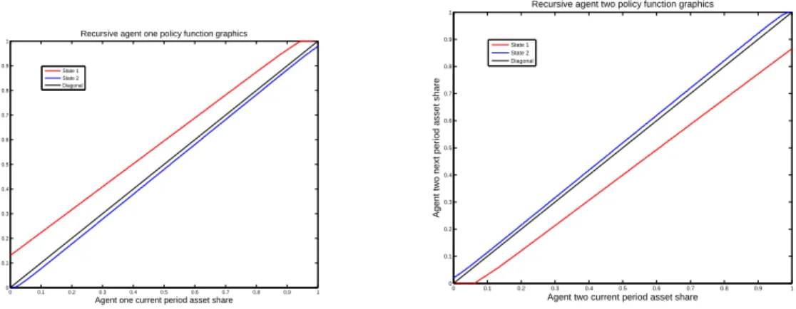
Figure 1: Graphics of ¯θ1 _7→θˆ1_(¯θ1_,1−θ¯1_{) and ¯θ}2 _7→θˆ2_(1−θ¯2_,θ¯2_{) fore}1_{(z) = p1}

and λ2_{(z) =p2 for all s∈ {z} 1, z2}

excess demand function ˆξa_{, with the proportionality constant chosen}

ap-propriately to ensure the speed of convergence; we compute again ˆθ′′ ₌

{θ˜i_(¯θi_{,θ, z,}¯ _θˆ′_,qˆ′_)}

i∈I for all (¯θ, z)∈gridS and repeat the previous step until

the desired precision. Notice that the convergence of the algorithm implies that the increment ∆ˆq′ _{is near zero and therefore the excess demand ˆξ}a _also

tends to zero in the limit.

We suppose that agents have homogeneous beliefs λi _{= λ and}

heteroge-neous instantaheteroge-neous income ei _{: Z → R}

++ depending on the states of the

nature. The budget set becomes for i= 1,2

Bi_(θi

-, z, q) ={(ci, θi)∈Ci×Θi :qcci+qaθi ≤(qa+qcdˆ(z))θi- +qcei(z)}

and we choose e1_(z

1) = 1, e1(z2) = 1, e2(z1) = 1 and e2(z2) = 2 that

is, this example includes aggregate risk on the income. Type 1 has initial asset endowment θ1

0 = 0.1 and type 2 has initial asset endowment θ01 = 0.9.

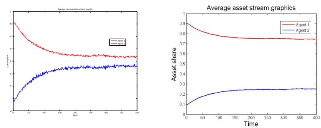
As a result we get linear affine policy functions and the dynamics of the simulations shows that all agents survive and the consumption and asset stream eventually becomes a stationary process. Figure 1 shows the policy functions. It is clear graphically that these functions are linear affine.

Figure 2: Graphics of ¯θ1 _7→qˆ(¯θ1_,1−θ¯1_{, z}

1) and ¯θ1 7→qˆ(¯θ1,1−θ¯1, z2)

0 50 100 150 200 250 300 350 400 1.9

2 2.1 2.2 2.3 2.4 2.5 2.6 2.7

Time

C

o

n

s

u

m

p

ti

o

n

Average consumption stream graphic

Agent 1 Agent 2

Figure 3: Graphics of the asset average stream P_r≤5000(ci

1t)(zrt)/5000 for

i= 1,2 on the left,P_r≤5000(θi

2t)(zrt)/5000 for i= 1,2 on the right, r= 5000

trajectories of (zr1, zr2, ..., zrT), T = 100 and λ2(z) = p = (0.4,0.6) for all

6

Conclusion

There exists a recursive equilibrium with minimal state space implementing a sequential equilibrium arbitrarily closed to a Magill Quinzii competitive equi-librium. Therefore, if agents update the recursive statistics with arbitrary small errors then, in the long run, they are close to the behavior of compet-itive equilibrium models presented in Radner (1972) or Magill and Quinzii (1996) with intertemporal consistency, even basing their choices in anticipa-tion of approximate future prices using continuous statistics with minimal state space to compute the equilibrium. We conclude that the transition functions of the recursive equilibrium represent an important instrument of coordination among agents if the measurement errors become small enough to avoid that agents deviate from their previous plans. Moreover, it is pos-sible o compute the approximate recursive equilibrium without using the first order conditions of optimality, through a method of iterating functional equations.

7

Appendix

Notation 7.1. Recall that L={1,2, ..., L}. ConsiderZ, Xi _⊂RL

+,Q ={q ∈

RL

+ :

P

l∈Lql = 1}, Q◦ = Q∩R++L , Qγ = Q∩[γ,1]L and S a topological

space. Define Xbi _{as the set of all bounded continuous functions ˆx}i _{:S →X}i

and Qb the set of all bounded continuous functions ˆq:S →Q both endowed with the topology induced by the sup metric. Define Qb◦ _{analogously. The}

absence of the upper index stands for the Cartesian product on i ∈ I and we write 1= (1,1, ...,1)∈RL

+.

Lemma 7.2. Suppose that Xi _{⊂ R}L

+ is a compact convex set with 0 ∈ Xi

and that Wi _{= R}L

+. Let Bei : Wi ×Q◦ → Xi be the budget correspondence

defined by

e

Bi(wi, q) ={xi ∈Xi :qxi ≤qwi}.

Then Bei _{is continuous.}

Proof: If Xi _{={0} is trivial. Suppose that X}i _{6={0}. The upper}

hemi-continuity follows from the fact that Bei _{has closed graph and compact range}

space. To show the lower hemicontinuity, let (wi

n, qn) ∈ Ai converging to

Suppose first that ¯qw¯i _{>0. Then there exists an open set}25 _{O of A}i

con-taining ( ¯wi_{,q¯) such that qw}i _{> 0 for all (w}i_{, q) ∈ O. Let IntB}ei _{: O → X}i

be the correspondence defined by IntBei_(wi_{, q) = {x}i _{∈ X}i _{: qx}i _{< qw}i_}.

Since 0 ∈ Xi_{, IntB}ei _{is nonempty on the set O and X}i _{is convex, then}26

e

Bi_(wi_{, q) = cl[IntB}ei_(wi_{, q)] for all (w}i_{, q) ∈ O. Clearly, IntB}ei _{has open}

graph. Therefore, using that an open graph correspondence is lower hemi-continuous and that the closure of a lower hemihemi-continuous correspondence is lower hemicontinuous, we conclude that Bei _{is lower hemicontinuous on O}

and hence there exists an N ⊂ N _{and a sequence}27 _xi

n ∈Bei(win, qn) for each

n ∈N such that xi

n →x¯i as n→ ∞.

If ¯qw¯i _{= 0 then ¯x}i _{= 0. Since ¯q}

1 > 0, 0 ∈ Xi and Xi is convex non

degenerated, there exists N ⊂ N _{such that q1n > 0 and (qnw}i

n/q1n,0) ∈ Xi

for n ∈ N. Choose the sequence xi

1n = qnwni/q1n and xiln = 0 for l > 1 and

n ∈ N. Then xi

1n = qnwni/q1n → q¯w¯i/q¯1 = 0 and hence xin → x¯i = 0 as

n → ∞. Moreover, by construction,xi

n∈Bei(wni, qn) for each n∈N. ✷

Lemma 7.3. Consider Y , Ye metric spaces with Ye compact and Ye ×Y en-dowed with the product topology. Suppose that f :Ye×Y →RL _{is continuous.}

Let C(Y ,e RL_{) be the space of all bounded continuous functions h : Y}e _{→ R}L

endowed with the sup norm. Then the function g :Y →C(Y ,e RL_{) defined by}

g(y)(·) =f(·, y) is continuous.

Proof: Consider a sequence yn → y and fix ǫ > 0. Then the set Y′ =

{yn}n∈N∪ {y} is compact. Therefore, f is uniformly continuous on Ye ×Y′

and hence the exists δ >0 such that for all ˜y,y˜′ _∈Ye

d((˜y′, y′),(˜y, y))< δ and y′ ∈Y′ implies||f(˜y′, y′)−f(˜y, y)|| ≤ǫ.

Assuming that28 _d((˜y′_{, y}′_{),(˜y, y)) = d}

e

Y(˜y

′_{,y˜) + d}

Y(y′, y) then choosing n0

such that n ≥ n0 implies dY(yn, y) < δ we conclude that n ≥ n0 implies

d((˜y, yn),(˜y, y))< δ for all y∈ Ye and hence ||f(˜y, yn)−f(˜y, y)|| ≤ǫ for all

˜

y∈Ye. Thus f(·, yn) converges uniformly to f(·, y). ✷

25

Recall that we are using the relative topology.

26

To see the inclusion Bei_(wi_{, q) ⊂cl[IntBe}i_(wi_{, q)], given x}i _{∈ Be}i_(wi_{, q) notice that if} we choose ˜xi _∈IntBei_(wi_{, q) then x}i

n := (1−1/n)xi+ ˜xi/n∈IntBei(wi, q) andxin →xi. Thusxi_∈cl[IntBei_(wi_{, q)].}

27_{The setN is chosen such that (w}i

n, qn)∈O for eachn∈N.

Lemma 7.4. Consider Y ⊂ Rn_{. Suppose that f : Y → Y and g : Y → Y}

satisfy f ∈ Lp(Mf) and g ∈ Lp(M g). Then f ◦g ∈ Lp(MfMg). Moreover,

if f ≤ νf and γg ≤ g ≤ νg for n = 1 and νf, νg, γg > 0 then h = f /g ∈

Lp(νgMf +νfMg)/γg2), the sum f+g ∈Lp(Mf +Mg) and the product f g∈

Lp(νgMf +νfMg).

Proof: Fix y, y′ _{∈ Y. Thus ||f(g(y))−f(g(y}′_{))|| ≤ M}

f||g(y)−g(y′)|| ≤

MfMg||y−y′||. Moreover, for n= 1

|f(y)g(y′)−f(y′)g(y)| ≤ |f(y)g(y′)−f(y′)g(y′) +f(y′)g(y′)−f(y′)g(y)| ≤ |g(y′)||f(y)−f(y′)|

+|f(y′_{)||g(y)−g(y}′_)|

≤(νgMf +νfMg)|y−y′|.

Therefore,

|h(y)−h(y′)|=|f(y)g(y′)−f(y′)g(y)|/|g(y)g(y′)|

≤ |y−y′|(νgMf +νfMg)/|g(y)g(y′)|

≤(νgMf +νfMg)|y−y′|/γg2.

Furthermore,

|f(y)g(y)−f(y′_)g(y′_{)| ≤ |f(y)g(y)−f(y}′_)g(y)

+f(y′)g(y)−f(y′)g(y′)| ≤ |g(y)||f(y)−f(y′)|

+|f(y′)||g(y)−g(y′)|

≤(νgMf +νfMg)|y−y′|.

✷

Lemma 7.5. Define m : RL _→ R _{by m(ξ) = max{ξk : k ∈ L}. Then}

m ∈Lp(1).

Proof:Take anyξk such thatξk =m(ξ). Thenm(ξ) =ξk ≤ |z−z′|+ξk′ ≤

|z−z′_|+m(ξ′_{) and hence m(ξ)−m(ξ}′_{)≤ |z−z}′_{|. By other hand, choosing}

ξ′

k such that ξk′ = m(ξ′), then m(ξ′) = ξk′ ≤ |z −z′|+ξk ≤ m(ξ) and thus

|m(ξ)−m(ξ′_{)| ≤ |z−z}′_{|. Therefore, m ∈Lp(1).}