•
i
•
セ@
..
PIEPGE SPE
V443e
セN@
F U N D A ç Ã O
GETULIO VARGAS
Lセ@
FGV
EPOE
SEMINÁRIOS DE PESQUISA
ECONÔMICA DA EPGE
lhe evolution of international output
differences (1960-2000): From factor to
productivity
FERNANDO
A.
VELOSO
(Faculdades IBMEC/RJ)
Data: 11/11/2004 (Quinta-feira)
Horário: 16 h
Local:
Praia de Botafogo, 190 - 110 andar
Auditório nO 1 Coordenação:
•
The Evolution of International Output Differences
(1960-2000): from Factors to Productivity*
Pedro Cavalcanti Ferreira (EPGE/FGV)t
Samuel de Abreu Pessôa (EPGE/FGV)
Fernando A. Veloso (Faculdades Ibmec/RJ)
June 2004
Abstract
This article presents a group of exercises of leveI and growth decomposition of output per worker using cross-collntry data from 1960 to :2000. It is shown that at least llntil 197.5 factors of production (capital anel education) ",ere the main source of output dispersion across ecoIlomies and that productivity variance was considerably srnaller than in late years. Qnly after this date the prominence of productivity started to sho\\' up in the data. as the majority of the litcrature has found. The gro\\'th decomposi-tion exercises showecl that t he reversal of relative irnportance of proeluctivity vis-a-\'is factors is explainecl by the very good (bad) performance of procluctivity of fast (slow) growing cconomies. Although growth in the pcriod, on avcragc. is mostly clue to factors accumulation. its variance is explained by productivity.
1
Introd uction
It is a well known fact that differences of output per workcr across countries are very high.
For example, in 2000 the average worker in the D.S. produced 33 times more than a worker
.. in Dganda, 10 times more than one in India, and almost twice as much as one in Portugal.
Dnderstanding the nature of output-per-worker differences across countries ShOllld be
... one of the main objectives of the literature of economic growth. since the leveI of output
*1'he authors ackllowledge the financiaI support of Cl\Pq-Brazil anel PRO:\'EX.
tCorresponding authar. Graduate School of ECOllOlllics. Fundação Getulio Vargas. Praia de Botafogo 190. 1107. R io de .Janeiro. R.J. RRRLGゥZセMYPPN@ Brazil. Email acldressesoftheauthorsare.respectiwly.ferreiraclJgv.br. pessoaÜfg". hr. fveloso.lt:iblllecrj. br
•
•
..
per worker of a glven country can be thought of as the result of its cumulative growth experience. Several authors have decomposed output per worker into the contribution of inputs and productivity, using different methods. In the early nineties, a few studies, e.g., \lankiw, Romer and \Veil (1992) and \Iankiw (1995) presented evidence that factors of production account for the bulk of income differences across countries.1 Recent papers by
Klenow and Rodriguez-Clare (1997), Prescott (1998), Hall e Jones (1999) and Easterly anel Levine (2001), among others, hmvever, have established what now seems to be a consellSUS that total factor productivity is more relevant than factors of production in explaining output differences .
This paper takes development decompositioll seriously. \Ve redo the main exercises of the literature for all years between 1960 anel 2000 (and not only for one single year, which is 1985 01' some year later in most articles in the literature). \Ve use a neoclassical production
function with a \Iincerian (e.g., rvIincer (1974)) formulation of schoolillg returns to skills to model human capital.
It turns out that the picture for earlier years is very different from the one that emerged from the literature. From 1960 to as late as 1975 factors are the ma in source of output per worker dispersion. By the mid-eighties, factors and productivity have roughly the same importance and from 1990 on productivity explains the bulk of international differences in output per worker. B.y 1960 the correlatioll of productivity with output per \vorker (in log terms) is 0.22, whereas the correlation of the latter with factor inputs is 0.71. Forty years later. the correlation of output per worker \vith produc:tivity jumped to 0.74. \vhile its correlatioll \vit h factors diel not change significallt ly. 2
The relevant questiono thus, is how one gocs from a worlel where, at least until 1975. differences in output leveIs are largely due to elifferenccs in physical anel human capital. to one where productivity plays the leaeling role. Om results shmv that one important reaSOll is that there \vas a strong process of convergence of factors of proeluction. anel of thc capital-output ratio in particular. Spec:ifically. t he variallce of factors of proeluction was nearly cut in half between 1960 and 2000.
Another way to tackle this qucstion is via growth elecomposition exercises for the sample countries. The results show that the illcrease in the capital-output ratio anel the eelucational
1 The view that factors of proeluction, anel physical capital in particular. are the main eletenninants
of differences in output per worker across countries has been labellecl in the literature either ét.'l .. capital
fUllelalllentalism" (e.g .. King anel Levine (1994)) or "neoclassical grmvth revi\'al" (e.g .. Klenow anel Roelrigllez-Clare (1997)).
2In 1960. the correlation of output per worker with the capital-output ratio anel 11ll11lan capital per workcr was equal to 0 .. )7 anel 0.72. respectively. By 2000. the correlation of outpllt per worker with the capital-outpllt ratio anel human capital was equal to 0.61 c 0.86. respcctively. \vhcreas its corrclation with factor inputs (capital-output ratio anel lmman capital comhincd) was 0.79.
,
•
leveI of the labor force explain the mean grO\vih of output per worker from 1960 to 2000,
whilc the behavior of productivity explains the variance of growth rates in the period. In
particular. inputs explain 80o/c of the gro\Vih of output per worker. whereas productivity explains 129o/c of the variance of the growth rate of output per worker.3 That is, capital deepening and human capital accumulation are general phenomena experienced by most countries. However. good (bad) growth performance is, in great measure, explained by high (low) productivity growth. In conjunction with the convergence of factors of production, this is the ma in reason behind the change in the pattern of income leveI decomposition.
Some particular experiences are helpful in the understanding of this fact. In 1960, pro-ductivity in Latin America was very dose to that of the leading economies. a fact often neglected in the literature. It was, on average. 182% higher than average produc:tivity of the "Asian Tigers"J. Forty years later. after having fallen 9o/c, productivity in Latin America was way below that ofthe industrial economics anel 337c smaller than the avcrage level ofthe Asian Tigers. At the same time, as a group, the Latin American economies had the second worst proeluctivity grcnvth rccord in the world. In contrasto productivity in thc East Asian ec:onomies grew at an annual rate which is alrnost 3 perc:entage points above the world aver-age. Not surprisingly, these countries are among the fastest grO\ving economies in the period. In other words. gnmih mirades (elisasters) are mostly productivity miracles (elisastcrs).
The paper is organized in five sections ill addition to this introeluction. III the next sectioll ,,-e present the methodology of alI exercises, the data anel calibration procedures. Scction 3 presents thc results of the level elecompositioll exerc:iscs anel Sec:tion 4 those of the gTowth ac:counting exercises. Section 5 further explores these results and disc:uss the performance of Latin America and fast growing Asian econornif's. Scction 6 concludes.
2
Model Specification, Data and Calibration
2.1
Madel
Let thc production function be given by:
,r
r..ro.( 4. L H ) ャセq@li!
=
l \ . i l ' it 11 it • (1):"The VariallCe af prodnctivity growth Illay cxceed the \"ariance af the gro,,"th rate af antpnt per ",arker elne to the llegatiw covariance between factors anel prodllcti\"it\" gro",th between 1960 anel 2000. See Sectioll 4 for detaib.
セ@ Sillgapore. Korea. Hong KOllg. Japall. Thailand allll Tai\\"all.
where lit is the output of country i at time t, K stands for physical capital, H is human capital (education) per worker, L is raw labor and A is labor-augmenting productivity. Notice thaL in this specification, total faetor productivity (TFP) is given by A;t-C>.
We use a ::\Iincerian (e.g., ::\1incer (1974) and \Villis (1986)) formulation of schooling returns to skills to model human capitaL H. There is only one type of labor in the economy with skill leveI detennined by its educational attainment. It is assumed that the skill leveI of a worker with h years of schooling is H = exp cp(h) greater than that of a worker with no
education, leading to the following homogeneous-of-degree-one production function:
Our first objective is to understand the relative contribution of inputs and productivity to international differences of output per worker in each year of our sample. The main question here is if the prominent role playecl by procluctivity in recent perioels is also a feature of previous years. In that sense, 41 variance-decomposition exercises, for the years from 1960 to 2000, are performecl. "Ve follO\v Klenow anel Roelriguez-Clare (1997) and Hall and Jones (1999), among others, re\\Titing the per worker production function in terms of the capital-output ratio. This formulatioll allows elecomposillg the variation of capital-output per workcr into variations of productivity, humall capitaL anel the capital-output ratio. In this sense, the production function is rcwritten as:
Y
(K
)
(1<"0) _ "71
=
セ@=
4 _.zt o(j)(hit )=
4. lC(l-Q'có(h,t) .:"t L. . I t ) T '-' • It"lt '-' .ti lt
where rt is the capital-output ratio. Taking logs of (2):
Q
In Yit
=
In At+
- - I n l-o: rtit+
o(hit ).(2)
(3)
Our scconcl objective is to stucly the relative contribution of factors anel productivity to the growth performance of countries. \Ve start frorn cxpression (3) above to obtain thc following growth decornposition expression between two arbitrary periüels:
o:
セ@ In Y
=
セ@ In A+
--.6. In t\+
セッHィIL@l-o: (4)
where .6. is the variation in a given variable between two periods. The relative contribution
•
of, say, productivity to the growth of output per worker is trivialIy given by:
セャョa@
セ@ In y ,
The advantage of the decomposition above with respect to the traditional growth account-ing procedures is that the accumulation of capital induced by an increase in productivity wilI be rightly attributed to productivity growth. l\Ioreover, this decomposition aIs o alIows us to assess to what extent the trajectory of a given economy refiects transitional dynamics or a balanced growth trajectory. In particular, the neodassical model predicts that. in balanced gwwth, the relative importance of capital deepening is nulL that is:
セセャョヲ|@l-o,
O
- - - - = ,
セャョケ@
Hence. depending on the value of the expression above we can assess how far or how dose any given economy is from a balanced grO\vth path.
2.2 Calibration and data
The specification ofthe function q;( h) takes into account international evidence (e.g., Psacharopou-los (1994)) of a positive and diminishing relationship bet\veen average schooling and return to education. Hence, instead of the more usual linear return to education we follow Bils and Klenow (2000) and set the (j) function as:
e
l 'q;(h)
= --,
fi -v.1 - I ) (5)
According to their calibration, we have i'
=
0.58 ande
=
0.32. In addition to these parameters we need to set the values of O: and b. the clepreciation rate used to construct the capital series. For (1, we use 0.40: estimates in Gollin (2002) of the capital share of output for a variety of countries fluctuate arouncl this value, a number also dose to that of the American economy according to the l\ational Income anel Product Accounts C:\IPA).\Ve use the same depreciation rate for alI economies, which was calculated from US data. \Ve employed the capital stock at market prices,G investment at market prices. l, as welI as
'> See Fraullleni (1997) for details 011 the met hodology nsed iIl the :"JIPA for t he estimation of the LTS capital
stock. The basic ide a is to use past investmcnt clata and secondary markct prices. at a high clisaggregation leveI. to calcnlate the valne of different t,\'pes of capital. The total capital stock at market prices is obtainecl as the result of th(' aggregatioIl of these scril's.
the law of motion of capital to estimate the implicit depreciation rate according to:
From this calculation, we obtained 6 = 3.5% per year (average of the 19,50-2000 period).
We used data for 83 countries during the period 1960-2000.6 Data on output per worker and investment rates were obtained from the Penn-\Vorld Tables (P\VT), version 6.1.' \Ve used data on the average educational attainment of the population aged 15 years and over, interpolated (in leveis) to fit an annual frequency, taken from Barro and Lee (2000).
The physical capital series is constructed with real investment data from the P\VT using the Perpetuai Inventory Method. In this case wc need an estimate of the initial capital stock. \Ve approximate it by Ko
=
10/[(1
+
g)(l+
n) - (1 - 6)1: where Ko is the initialcapital stock, lo is the initial investment expenditure, 9 is the rate of technological progress
and n is the growth rate of the population.8 In this calculation it is assumed that a11
economies were in a balanced growth path at time zero. so that Lj
=
(1+
7I)-j (1+
g)-j lo.To minimize the impact of economic fiuctuations we used the average investment of the first five years as a measurc of lo. \Vhen data \\las available we started this procedure taking 1950 as the initial year in order to reduce the effect of Ko in the capital stock series.9 \V'e obtained the rate of technological progress by adjusting an exponential trend to the U.S. output per worker series. correcting for the increase in the average schooling of the labor force and obtained 9 =1.5370. The population growth rate. n, is the average annual growth
rate of population in each economy between 1960 and 2000. calculated from population data in the P\VT.
In order to compute the value of Ait, we use the obscrveel values of Vit anel the constructed
6Sec the Appendix for a Iist of the countries indudec! in the samplc. For some coulltrics. we elo not ha\"e data for either 1960 or 2000. but tl1(>:" \\"ere still includcd. In particular. \\"c llsl'd 1961 as thc initial ycar for Tunisia. For a fe\\' cOllntries. we used a year othe1' than 2000 as the last :-"ear. namely Cyprns (1996). Congo (1997). Central African Republic anel Taiwan (1998), Gu:-"ana. Papua New Guinea. Fiji anel Botswana (1999).
'For lllore eletails Oll this \"ersion of the Penn-\Yorlel TaLle. see Heston. SUIllIllers allel Atten (2002)"
セtィゥウ@ is the discrete time wrsion of the formula used in King and Le\"ine (1994) anel Hall anel Jones (1999). aIllong othe1's.
9For some ecoIlornies this proceelure to calculate the initial capital stock in 1950 yields capital-output ratios far abo\"e the obser"eel ratio in the CS. At the sarne time the marginal proclucti\"it:-" of capital is \"<:'r:-' lo\\' whl'n we use this llleasure of the initial capital stock. This results frorn the fact that Japan anel sl'\"eral countries in Continental Europl' hael \"ery high invcstmcnt rates in the early fifties. <luc to the reconstruction efIort after the Second \Yorld \Var. In these cases \\"e constructcel an altcrnati\"c nwasnrc of Ko so t hat the marginal proelucti\"ity of capital in 1950 was RPッONセ@ aLove that of the lj.S .. This \"alue of the PJ[yK seems high enough in order to be consistent with the investment rates obscrved in the post-war pcriod anel prevents the capital-olltpllt ratio from decliniug in some conutries. The resnlts are qnalitati\"ely similar to the ones reported in the texto SOllle results Laseel ou this measure are reporteel in tbe Appendix.
..
series of /'Lit and H it so that the productivity of the i-th economy at time t was obtained as:
(6)
Using the constructed values of /'Lit, we can also compute the marginal product of capital
as:
(7)
3
Development Accounting
In this section we perform development accounting exercises, based on variance decomposi-tions of output per worker for each year from 1960 to 2000. In most of our calculations we follow Klenow and Rodriguez-Clare (1997) and compare the contribution of X, a compositc
セ@ (} l-D
of the two factors (i.e., Xit
=
/'Lit U e 1_,;,1l.t ), with that of productivity. From (3), we have:In Yit
=
In A it+
In X it . (8)However, as opposed to these authors, wc elccomposc thc variance ofln(y) accoreling to its mathematical expression, allowing for a covariance term between factors anel proeluctivity:
(9)
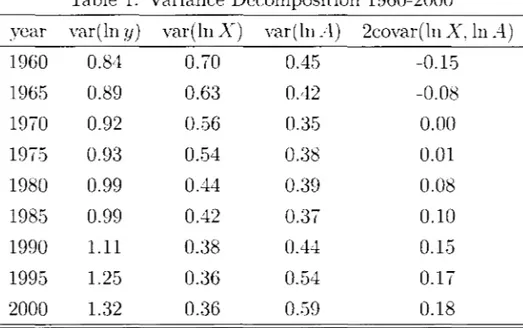
This is important in thc prcscnt contcxt because, as we ,:I/ill see shortly, the covariance component has a markeel change of behavior in the perioel, so that leaving it out would imply eliscareling an important piece of information about the nature of output elispersion.10 Figure 1 elisplays, for each year of our sample, the participation of the 3 components of the variance of (the log of) output per worker. Table 1 presents the values of all the components of expression (9) at five-year intervals.
IOThe variance dccomposition formula used 「セG@ Klenow and Rodrigllez-Clarc (1997) is gi\'en hy ('ur(ln y,r) =
c01'(lnYif,lnAi/) + cor (lnYi!.lnXitl. In terms of (9). this amounts to dividing the covariance term cor(ln Ait • In XII) eqllall,\' hctwecn thc "ariance terms. por (In Ail ) and ror (In Xid. In the Appendix. we
present results for thi5 variance decompositiüu.
.,
MMMセ@ ...
-NAャNNセ。イHォhI@ • variA) []2*covar(kH,A)
Figure 1: Output per worker variance decomposition - 1960-2000
Figure 1 and Table 1 reveal a number of interesting facts, First, output per worker dispersion increases throughout the period, espec:ially in the nineties, In particular, the variance of (the log of) y increR..'ied from 0,84 in 1960 to 1.11 in 1990 and 1.32 in 2000. Second, there is a continuous reduction of the absolute importance of factors in accounting for output dispersion. Between 1960 and 2000. the variance of (the log of) X declines nearly 50%, from 0.70 to 0.36. Hence, while it is observed a strong process of output divergence, factor leveis c:onverged.
Table 1: Varianc:e Decomposition 1960-2000
year var(1n y) var(1n X) var(ln A) 2covar(ln X, In A)
1960 0.84 0.70 0.45 -0.15
1965 0.89 0.63 0.42 -0.08
1970 0.92 0.56 0.3,5 0.00
1975 0.93 0.54 0.38 0.01
1980 0.99 0.44 0.39 0.08
1985 0.99 0.42 0.37 0.10
1990 1.11 0.38 0.44 0.15
1995 1.25 0.36 0.54 0.17
2000 1.32 0.36 0.59 0.18
•
during the period. In 1960 the contribution of the vanance of factors of production to the variance of output per worker was 55% higher than that of productivity. By the mid-eighties the variance of factors and productivity had roughly the same importance, whereas in 2000 factors variance wa.'3 39% smaller. It should be noted that in 1985 X and A had approximately the same importance as sources of output per worker dispersion.
Finally. the covariance between factors and productivity increases continually. As a matter of fact, it changes signs, going from from -0.15 to 0.18 throughout the period. This means that in 1960 those economies that displayed high productivity \vere not necessarily those with high factors endowment, but by 2000 productivity, capital intensity and education were positively correlated across countries.
Figures 2 and 3 display productivity leveIs, relative to the US, plotted against relative output per worker in 1960 anel 2000. As the figures show, the relationship hetween the two variables is much weaker in 1960 than in 2000. Specifically, the coefficient of a simple OLS regression of relative productivity on relative output per worker is only 0.05 (R2
=
0.0005)in 1960, whereas in 2000 the regression coefficient is 0.76 (R2 = 0.47).11
1-75
L.5
L2·5
セ@ 1
0.7.5 0.25
•
•
•
• $•
•
•
•
•
••
•
•
.... t • •
•
•
..
.
·
• # ...
..
• •.
....
...
セ@ セNNN@.
•
•
• •
l 4J ••
•• • Std. E:r:r. =0. 26
.... ... Coeff. =0. os • R2=0.000S
o 0.2 0.4 0.6 0.8 1 1 .,
Y
Figure 2: 1960
1-75
•
1-5•
1.25 0.75 O.S 0.25o 0.2 0.4 0.5 0.8 1 1.2
Y
Figure 3: 2000
The picture that emerges from the results above is one where in 1960 the variability of productivity was lower and that of factors was higher. In contrasto throughout the period, there was a strong process of convergencc of factors of production. \loreove1', cspecially after the mid-eighties, the variability of productivity increased. This result, in a certaiu
11 In 1975. the cross-countr:-' relatioIlship het\\'ccIl relativc proeluctivity anel rclative ontput per worker is
wcak. In particular. the rcgression cocfficicnt is O.3..! (R2 = 0.05). This suggcsts that the ]"l'sult that thi"
rclationship becamc stronger ovcr time is not an artifact of thc method \H' uscd to C"OIlstrnct t he initial
capital stock.
sense, qualifies the literature on international differences in leveIs of output (Klenow and Rodriguez-Clare (1997), Prescott (1998), Hall and Jones (1999) and Easterly and Levine (2001), among others), whose main finding is that productivity differences account for the bulk of the dispersion of output per worker across countries. \tVe find that this is a recent fact: in 1960 quite the opposite occurred, and factors, not productivity, explained most of the output per worker variation.
Take for instance the BK3 decomposition of Table 2 m Klenow and Rodriguez-Clare (1997). It was calculated using 1985 data and the production function and human capital formulation were similar to the one \\'e use. They found that factors explained 537c. of output per worker variance and productivity the remaining 477c. If we lL.'3e the variance decomposition formula used by theses authors, we obtain very similar results. Specifically, the relative importance of X and A in 1985 were equal to 52% and 48%, respectively (see the Appendix for the calculations)Y However, the result is very different \vhen we use 1960 data: 64% of the output variance is explained by factors. This result is reversed in 2000, when productivity accounts for 58% of output per worker dispersion.
It should be noticed that there is nothing essentially wrong \vith previous results. Our point is that one cannot generalize them to early years. The relevant question is hmv one goes from a \vorld where. at least until 1975, differences in output leveIs are largely due to elifferences in physical anel hurnan capitaL to one where productivity plays the leading role. This is \vhat we investigate in the next section.
4
Growth Accounting
In t his section we investigate t hc contribution of t hc various cornponcnts of t hc proeluction
fUllction to the growth experience, from 1960 to 2000. of 83 economics. \Ve use equation (4). so that the variation of the log of output per \vorker in the period is elecomposeel into the contribution of proeluctivityY the capital-output ratio and human capital per worker.
In 0UI" sample average output per worker went from US$ 10,033 ill 1960 to US$ 24,533 in
2000, growing 145% in the period.1
! Throughout this paper alI results for avcrages of a given
variable among countries \vere obtained frolIl geornetric averages of the given variablc across the relevant group of countries. Table 2 presents some elescriptive statistics using 1960 and
12If we take BK4 in Table 2 of Klenow anel Roelrigllez-Clare (1997) instead. the contribution of factors
aIlel proclllctivity in 1985 are 34 (7c anel 66%. イ・ウー・」エゥ|B・ャセᄋN@ which are doser to our results in 2000.
J:l As rnentioned above. it shoulcl be lloticed that T F P = A l-I). However. in the growth decornposition.
the COlltribution of TFP ís givell by the (log) variatioIl of A. which captures both the direct anti indírect (via capital accunmlation) effect of TFP on the growth rate of olltpllt per worker.
11 Ali figures are in 2000 values. correcterl for PPP.
2000 figures (we set A = 100 for the US in 1960):
Table 2: descriptive statistics (1960-2000)
Y60 Yoo
sample average US$ 10,033 US$ 24,533 66 85 1.69 2.24 2.4 6.0
In the last forty years mean productivity increased by 29%. On averagc, cconOllllCS became more capital intensivc, with an increase in the capital-output ratio of 33%. It was also observed a vigorous increase in education which jumps, on average, from 2.4 years in 1960 to 6.0 ycars in 2000.
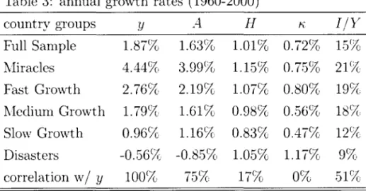
In order to further understand the role of productivity and factors on the international development process, another sct of stylized facts is presented in Table 3. \Ve divide thc economies in 5 groups, according to their growth rates of output per worker: in the economic :·Mirades" group (15 economies) the growth rate of output per worker ranged from 3.28% to 6.12% per ycar. in thc "Fast Growth·' group (14 cconomics), it ranged from 2.39% to 3.18%: in "Medium Growth·' (22 economies), from l.46% to 2.07%; in "Slow GrO\vth" (19 economies), from 0.61% to l.4.5% and in the economic :·Disasters" group (14 cconomies). thc average growth ratc ranged from -3.2.5% to 0.44% per year. This procedure is somewhat arbitrary but it serves to our purpose of calling attention to different patterns of development across ccononucs.
Table 3: ammal grO\vth rates (1960-2000)
country groups y A H 1\ J/Y I
Full Sample l.87% l.63% l.01% 0.72% 15%
IvIiradcs 4.44% 3.99% l.15% 0.75% 21%
Fast GrO\\!ih 2.76%, 2.19% l.07% 0.80% 19% :rvIcdium Growth 1.79% l.61% 0.98% 0.56% lSS{,
Slow Growth 0.96% l.16% 0.83% 0.47% 12%
Disasters -0.56% - . O "-% t;.') C> l.05% l.17% 9%
correlation w / y 100/() 759(, 17% 0% 51% note: I/Y in leveIs, not grO\\ih rates
The average capital-output ratio grew at 0.72% a year. while average productivity in-creased 1.63% annually. Table 3 shows t11at productivity grO\\!ih increases monotonically with the average growth rate of output per worker. \Vhile for the ·:ll/Erades'·, productivity grO\\!ih averaged 3.99% per year. for the "Disasters" the average growth of A was negative.
,
In fact, the correlation between gwwth of output per worker and productivity gwwth was very large in the period (0.75).
The correlation of output per worker growth with the investment rate was relatively smaller, 51%, although average I/Y increases monotonically, across groups, with the grmvth rate. ),loreover, the capital-output ratio raised in all groups, even in the "Disasters" cconomics
(which experienced the highest grmvth of the capital-output ratio). In fact, the correlation between the growth rates of output per worker and the capital-output ratio is dose to zeroY:; Table 3 also shows that average human capital increased 1.01% annually, but its correlation
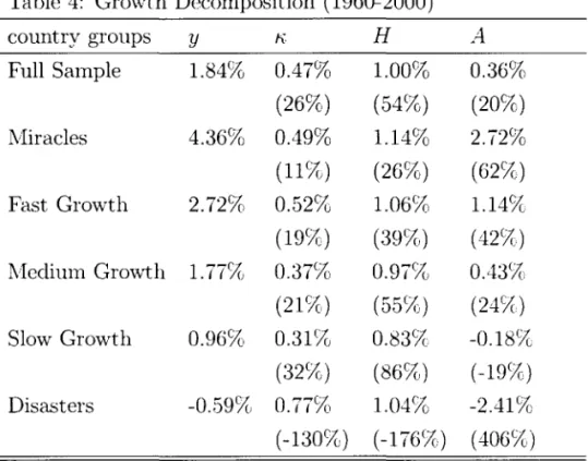
with y grO\vth is small (17%). In fact. the growth rate of H is very similar across groupsYi Table 4: Growth Decomposition (1960-2000)
country groups y K H A
Full Sample 1.84% 0.47% 1.00% 0.36%
(26%) (54%) (20%)
Mirades 4.36% 0.49% 1.14% 2.72%
(11%) (26%) (62){)
Fast Growth 2.72% 0.52% 1.06% 1.14%
(19%) (39%) (42%)
l'vlcelium Grm'v1:h 1.777cJ 0.37% 0.97% 0.437c,
(21%) HセセOゥZI@ 00 ü (24Vc.)
Slow Growth 0.96% 0.31% 0.83% -0.18%
(32%) (86%) ( -19%)
Disasters -0.59% O . I I
'"''"'o/c
o 1.04% -2.41% (-130%) (-176%) (406%).\"ote: Thc nurnbcrs in parcllthesis arc thc rclative cOlltributions of each factor to output per worker growth.
Tablc 4 presents thc growth decomposition exercises for cach group between 1960 anel 2000. The first linc of the table shows the important role played by factors to explain growth
rates. On average, 80% of the observeel growth of output per worker can be accounteel by
human and physical capital accumulation and only 20% is elue to productivity grov.rth.17
15This reslllt is similar to the obtained by Klenow anel Rodriguez-Clare (1997) for the period 1960-1985. They obtaineel a correlatiou of 0.04 betweeu the growth rate of Olltpllt per worker auel the capital-outpllt ratio.
lGThis result confirms the fiuclings of Benhabib and Spiegel (1994) and Pritchett (2001).
I 'Indepeueleut research by Baier. Dw.\-er . .lr. aud Tamura (2004) found a relative contribution of TFP for
output p(>r workcr growth of 149;' •. Their stucly ha.·, sewral differences from ours. First. they use data for a largcr sample of 145 countries. spanlling more than a hnndred years for 23 of those countries. Second. these
Human capital alone accounts for 54% of output per worker growth.1í:i
Notice, however, that the sample average hides a lot of information with respect to the behavior of different economies. In the faster growth group, the ":VEracles" econornies, 62%
of output growth is explained by productivity grovvth. This number falls monotonically with the average growth rate in each group: it is 42% in the "Fast Growth" group. 24% for
the ":Vledium Growers" and -19% for the "Slow Growers". For the "Disasters", the fall in productivity accounts for 406% of the decline in output per worker. In other words, economic rniracles were productivity rniracles. By the sarne token. poor perforrners in generaL and disasters in particular, had a very bad record of productivity grmvih.
Results in Tables 3 and 4 allow us to conclude that the increase in the capital-output ratio and the educational leveI of the labor force explain the mean growth of output per worker,]() while the behavior of productivity explains the vaTÍation of growt h rates among groups.
Another way to assess the importance of productivity for growth differences between countries is to perforrn a decomposition of the variance of the grO\vth rate of output per worker in terms of the variance of factors and productivity growth and the covariance between factors growth and A growth. Using (4), we can decompose the variance of output per worker growt h as follows:
vaI' HセャョNャOI@
=
カ。イHセ@ In A)+
カ。イHセ@ In X)+
R」ッャGHセ@ In A. セ@ In X). (10)Table 5 presents the variance decomposition results for the grO\vth rate of output per worker. The table shows that productivity growth accounted for the bulk of the variance of output per \vorker growth between 1960 and 2000. Specifically, the variance of A gTOwth accounted for 129% of the growth variance. whereas the variance of factors growth accounted
for only 3.5% of the dispersion of output per worker gTowth.20
authors use the standard growth decompositioll formula in which the growth rate of output per worker is related to thc growth rates of TFP, human capital per worker and ーィセBウゥ」。ャ@ capital per worker. instcad of the capital-olltpnt ratio. Third. in most of thcir calcnlations they nse weightcd avcragc growth rates. in whic:h thc weights are thc 」ッオョエイセBGウ@ labor force in 2000 and the nllmber of ycars for which data for the cOllntry ゥセ@ available. For the llnweighted rclative contrilmtion of TFP they obtain a startling \"alue of -1099:. which to the best of om kllowledge is illCollsistent with ali TFP studies for periods close to the one we c:onsider in this paper.
I セ@ OIle should rernember that we are accoullting as a cOIltribution of 111lrnall capital to outpllt per worker
growth the illcrease iu the capital-labor ratio due to the iucrease in the edncationallevel of the labor force. 19The result is similar if we use the TIIedwn insteacl of the mean. In particular. factors accunllllation account for 09% of mediall outpnt per worker growth between 1%0 anel 2000 [checar].
2oKlenow anel Rodriguez-Clarc (1997) fouucl that the \"arianc'e of procluctivity growth explains between 86% and 91 % of t hc \'ariance of outpnt per worker growth. The variance decomposition formula used by t lll'se allthors is given hy l'uT(6In y) = cov (61n y. 61n A)
+
em; (61n y. 61n X). In tcrms of (10). this amountsTable 5: Variance Decomposition of Growth Rates
period カ。イHセャョケI@ カ。イHセャョxI@ カ。イHセャョaI@ R」ッカ。イHセ@ In X, セ@ In A)
1960-2000 0.51 0.18 0.66 -0.32
1960-1970 0.05 0.02 0.10 -0.07
1970-1980 0.07 0.04 0.12 -0.09
1980-1990 0.06 0.02 0.09 -0.05
1990-2000 0.05 0.02 0.08 -0.05
From Table 5 we can aIs o observe a negative covariance between the growth rates of A
and X between 1960 and 2000. In particular, the correlation between the gwwth rates of A
anel the capital-output ratio was -0.51 in this period. This negative correlatioll is observed in each decade and may indicate an overstatement of the contribution of K to output per worker growth.21
Easterly (2001) documents the fact that in the period 1980-1998 median per capita income growth in developing countries was 0.0 percent, as compareel to 2.5 percent in 1960-79. This occurreel despite the fact that several variables that are supposed to ellhance growth improved over the latter period, such as health, education, fertility, infrastructure and macrocconomic variables. including the inftation rate and the degree of real overvaluation of local 」オイイ・ョ」セイN@
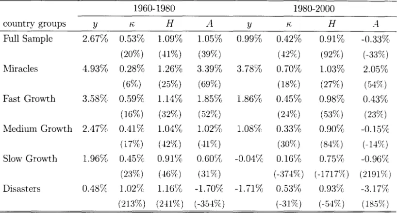
In order to assesss if this pattern is verified in our sample, we present in Table 6 growth accountillg results for two subperiods: 1960-1980 alld 1980-2000.22
Table 6 shows that there was in fact a significant growth slowdown after 1980. Specifically. average growth in the sample declincd from 2.67% in 1960-1980 to 0.99% in 1980-2000. From the table we call also observe that the fall in productivity growth \vas the main culprit of the growth slowdown. In fact, for the whole sample A growth was positive until 1980 (1.05% per year) anel bccame negative since then (-0.337rJ per year), whereas the growth rates of
to dividing the covariance term col'(D.ln A. D.ln X) eqnally between the variance terrns. ror (D.ln A) and
l'ar (D.ln X). Using t his formula. we obtain tltat the variance of A growth accounts for 979é of the variance of y growth between 1960 and 2000. In the Appendix, \\'e present results for this varinnce decomposition. Baier. Dwyer. .lr. and Tamma (2004) also obtain the イ・セョャエ@ that the variance of proeluctivity (TFP) ゥセ@ lIlore important than the variance of factors to explain the variation of growth rates.
21 Klenm\' anel Roelriguez-Clare (1997) obtain a correlatioll between the growth rates of A anel /'{ of -0,42. See their paper anel Pritchett (2000) for an cxplanation for this result baseel on nn overstaterncnt of thc contribution of the capital-output ratio elue to the fact that public investment is less efficient thall pri\'ate investmcnt in generating ーィセGウゥ」。ャ@ capital from a given Clmount of investment. 1\n alternatiw explanation baseei on the neoclassical growth model wonld bc that a decreêL'-;c in the grO\vth rate of productivity wonll! temi to increase the growth rate of thc capital-ontpllt ratio in thc transition to a ne\\' balanced growth path. 22Rodrik (1999) also dOCllll1ents that mauy conutries experiellced a growth collapse. but he dates the start of the growtlt slowdown to 1975 instead of 1980 as in Easterly (2001). Based on this, we also perforrned growtlt accouIlting exercises for the ウオ「ー・イゥッ、セ@ 1960-1975 allli197.1-2000. The results are qualitatively similar to the ones reported in the texto anti are available frOlIl tlte anthors npOll reqnest.
the capital-output ratio and human capital per worker declined much less. This pattern is also observed for all groups. In the period 1960-1980 only the disasters expcrienced ncgative
A growth, \vhereas in the subsequent period the "Slow Grmvth" and "lvIedium Growth" countries aIs o had an absolute decline in productivity.
Table 6: Grmvth Decomposition by Subperiods
1960-1980 1980-2000
country groups y
'"
H A Y K HFull Samplc 2.67% 0.53% 1.09% 1.0.5% 0.99% 0.42% 0.91%
(20%) (--11%) (397é) ( -!2%) (92%)
Miracles 4.93% 0.28% 1.26% 3.39% 3.78% 0.70% 1.03%
(6%) (25%) (69%) (18%. ) (27%)
Fast Grmvth 3.58% 0.59% 1.14% 1.85% 1.86% 0.45% 0.98%
(16%) (32%) (52%) (2-!%) (.53%)
Medium Growth 2.47% 0.41% 1.04% 1.02% 1.08% 0.33% 0.90%
(17%) (-!2% ) (-!19é) (30%) (84%)
Slow Growth 1.96% 0.45% 0.91% 0.60% -0.04% 0.16% 0.75/<',
(2:3%) (-!6% ) (:31 o/c) (-:37-!%) (-1717(7c )
Disasters 0.48% 1.02% 1.16% -1.70% -1.71% 0.53% 0.93%
(213%) (2-!1%) ( -35-!%) (-31 %) (-54%)
-:\ote: Thc numbers in parcnthesis are the rclative contributions of cach factor to output per worker growth.
A
-0.33%
( -33%)
2.05%
(54 o/r.)
0.43%
(23% )
-0.15%
(-14%)
-0.96%
(21919é)
-3.17%
(185%)
Summing up the results. capital deepening and human capital accumulation are general phenomena experiencecl by most countries. On the other hanel, gooel (bacl) growth perfor-mance is, in great measure, explained by high (low) productivity growth. In conjuntion with factors convergence. this is the ma in reason behinel the change in the pattern of output per worker levcl clecomposition clocumentcd in the previous section. In 1960, for historical reasons outside the scope of this article, inputs were the decisive difference bet\veen rich and poor countries. Between this date and the enel of the century fast growers anel most of the rich countries experienced a significant increase in proeluctivity, while slow growers and many poor economies laggecl behincl or even reeluced their productivity leveI, so that productivity variance increased significantly. Factors dispersion. in contrasto declined in the same period. Hence, in 2000 the relative contribution of productivity in explaining international income differences was vastly raised surpassing that of inputs.
5 The Performance of Cultural and Regional Groups
The role of institutions and cultural factors in the economic performance of countries has been the subject of an increasing number of studies in the fields of history and economics (e.g., North (1990), Engerman and Sokoloff (1994) and Acemoglu. Johnson and Robinson (2001). among many). In a way or another societies may choose or inherit sets of laws, institutions and social conventions that are more inductive to investment in business, technology and education and that perform better in protecting property rights and the fruits of these investments. In these countries, the incentives and productivity are higher, and so are investment and grO\vih.
In this section countries are divided in broad groups on a cultural or geographical basis. We have two objectives with this. First, we would like to understand better the evolution of productivity in the period, and the proposed group division may shed some light on this subject. Second, this division reveals growth facts neglected in the literature that \viU allow us to provide evidence related to some important questions. For instance, we found that as late as 1975 Latin America productivity was high by intemational standards, that
A grO\\ih subsequently was strongly negative and that rnost of the grm-vih in the region between 1960 and 2000 was via fadors accumulation. Countries in thc region may havc experienced transitional gTO\vth in that period. which has irnportant implications in terms of thcir future growth trajectory.
\Ve divided economies in 9 groups, which are presented in detail in the Appendix. Thcy are \Vestem Europe. South Europe, English (speaking), Asian Tigers, }Iiddle East. South Asia, Latin America. Caribe and Sub-Saharan aヲイゥ」HャNセ[ャ@ The first group has 12 countries that comprise most of \Vestern Europe, with exceptiolls sueh as Portugal and Spain (that belollg, together with Greece, Cyprus and Turkey to "South Europe") and Unitecl Kingdom. Thc latter bdongs to the "English" speaking group, which aIs o has USA, New Zcaland, Australia. Ireland and, less accurately, Canacla. Asian Tigers are Singapore, Korea, Hong Kong, Japan. Thailand and Taiwan. There are 5 and 10 economies. respectively, in the next two groups and 18 in the Latin America. which also includes Caribbean countries that speak lllostly Latin languages. The Caribe group contains ouly 4 countries and the Sub-Sahara cOlltains 17. Table 7 presents averages anel growth rates for some variables by cultural and regional groups (we still set A
=
100 for the US in 1960).Each cell displays cross-country geometric mcans of a given statistic in the group. \Vc can observe t hat t he Asian Tigers. on avcrage, experienced an extraordinary gnmi h of
2:'It should be rnelltionccl that om sample of Sllb-Saharan countries is ver:' illcomplete. as we did llot illcIude in our sample those economies for which data is availabIe onl:' after 1960.
productivity of 284% between 1960 and 2000. Whereas in 1960 the leveI of A for the Asian Tigers was only 35% of the correspondent value for "English Speaking" countries, by 2000 this ratio had increased to 77%. The big losers are Latin American economies and the Sub-Sahara region, with mean reductions of productivity of 9% and 34%, respectively. It should be noticed that this decline in productivity in Latin America occurred after 1975. The leveI of productivity in Latin America, at least until 1975, was dose to the one observed in the advanced countries. In 1960 it corresponded to 79% of the leveI of A in the US, whereas in 1975 it had increased to 88%. By the end of the century, however, this ratio had shrinked to 45%.2-1
Table 7: Average leveIs and growth rates (1960-2000)
country groups 6Y60-00 A1960 A 1975 A 2000 セaVPMPP@ 1'\1960 1'\2000 セQG|VPMPP@
English (speaking) 107% 80 105 138 72% 2.50 2.7.5 10%
Westem Europe 140% 74 107 131 76% 3.42 3.93 15%
South Europe 267% 55 93 114 109% 2.34 3.02 29%
Asian Tigers 636% 28 57 107 284% 2.08 3.30 59%
Middle East 149% 89 118 114 27% 1.81 2.01 11%
South Asia 162% 66 65 73 10% 0.97 1.71 76%
Latin America 42% 79 104 72 -9% 1.67 2.11 26%
Caribe 87% 46 66 73 59% 2.70 2.33 -14%
Sub-Saharan Africa 26% 67 63 44 -34% 0.86 1.37 60%
vVith the exception of the Caribbean countries, in all groups the capital-output ratio increased in the period. with the South Asian countries experiencing the biggest boost in capital intensity. The Asian Tigers and Sub-Saharan countries expcricnced an increase in fi. of 60%. There was an increase in the capital-output ratio even in groups, such as the ooEnglish Speaking" and vVestem Europe, where capital cleepening in 1960 was relatively high by intemational stanclarcls. This result confirms that the pcriocl between 1960 and 2000 was characterized by wiclespreacl factors accumulation, now taking cultural or geographical factors as our standpoint.
As a result of the significant 111crease 111 the capital-output ratio, the real return on capitaL as measurecl by the marginal procluct of capitaL::!;; dedinecl substantially for all
セセtィ・ウ・@ reslllts for Latin Arnerica are similar if \Ve consieler only the most poplllated countries in 2000 (Brazil. :\rexico. Argentina. Colombia. Peru. Venezuela anel Chile). Specificall,v. for this graup of Latin Arnerican COllntrics. thc vallles of A \Vere 7.') in 1960. 106 in 1975 and 74 in 2000.
2:ipritchett (2000) argues that pllblic investment is not rnea'iured correctly in the セ。エゥッョ。ャ@ Acconnts. which may lead to an overestimation of thc standard rneasnrcs of the capital stock. In this ca .. 'ic. our rnca .. 'inrc of
PjlgK may not be captnrillg the marginal impact of capital on ontpnt. bllt instead thc degree of efficiellcy
country groups between 1960 and 2000, converging toward a value between 10% and 22%, with the exception of the Sub-Saharan Countrics, which still had a very high real return on capital in 2000 (39%). Figure 4 presents the evolution of PAlgK for selected groups throughout the period. using the measure constructed using (7).
0,40
0,35 KMNNBLエAZN]セ[[ZZZM
__________ -..:.. ___________ _
0)0 +---'---""'0..---'---_-,--_ _ _
0,10
エ]]]]]]]]]]]]ZZZZZZ]]]Z[]]BBGMセセ]]]@
...
MMMMセ[[Z[[NLN@
0,05
I
0,00 "-I _ _ - _ - - - - _ -_ _ - - - _ - - - _ -_ _ _ MMセ@
]Mwセイャ、aカ・イ。ァ・セ@ English (Speaking) - Westcrn eオイッ{ャ・セM Asian tゥァ」セ]M Latin Arncrica
Figure 4: :\Iarginal Product of CapitaL Sclccted Country Groups (1960-2000)]
Table 8 surnrnarizes the growth decornposition exercises for each group. The methodology is exactly the same as that of Table 4. In the first four groups, from one half to oue third of the grO\vth of output per worker is due to A grO\vth. Thc contributioll of productivity for output per worker grO\vth is particularly high for the East Asiall Tigers, both in absolute and relative terms, a poiut to which we shaIl return belO\v. At the other extreme, Latiu America and Sub-Saharan Africa experienced a faIl in productivity throughout thc period, which was offset by the contributioIl of factors to growth.
of the goverlllllent in transforming investlIll'nt into Ilnits of physical capital. In an!' case. PJJyl\ wOllld still be a llleasnre of the real retllrn on investment.
Tablc 8: Growth Decomposition (1960-2000), Cultural
and Regional Groups
country groups y fi, H A
English (speaking) 1.82% 0.16% 0.51% 1.16%
(9%) (28%) (64%)
Westcrn Europe 2.17% 0.21% 0.72% 1.23%
(10%) (33%) (57%)
South Europe 3.33% 0.40% 1.25% 1.68%
(12%) (37%) (50%)
Asian Tigers 5.04% 0.78% 1.02% 3.24%
(15%) (20%) (64%)
Middle East 2.29% 0.17% 1.68% 0.4.5%
(7%) (73%) (199(, )
South Asia 2.41% 0.95% 1.32% 0.14%
(39%) (55%) (6%)
Latin America 0.87% 0.38% 0.93% -0.4.5%
(44%) (107%) (-51%)
Caribe 1.58% -0.25% 0.84% 0.99%
(-16%) (53%) (63%)
Sub-Saharan Africa 0.57% 0.80% 1.04% -1.26% (140%) (1809(,) (-222%)
.\"ote: The nurnbers in parenthesis are the relative contributions of each factor to output per worker growth.
5.1 The Latin America Stagnation
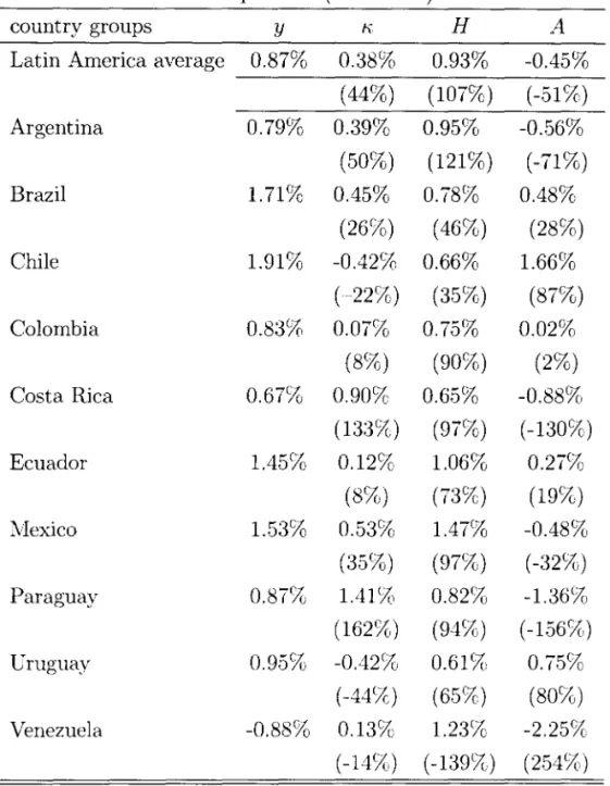
Thc growth dccomposition rcsults for sclcctcd Latin Amcrican cconomics prcscntcd in Tablc
9 reveal that most countries in the region experienced a decline in productivity between 1960
and 2000. and consequently growth was mostly due to factors accumulation. One exception
is Chile. which had a significant increase in A. On the other hand. the fall in productivity in Venezuela and Paraguay was particularly strong.
Table 9: Grmvth Decomposition (1960-2000)- Latin America
country groups y K H A
Latin Amcrica average 0.87% 0.38% 0.93% -0.45%
(44%) (107%) (-51%)
Argentina 0.79% 0.39% 0.95% -0.56%
(5070) (121%) (-7170)
Brazil 1.71% 0.45% 0.78% 0.48%
(26%) (4670 ) (28%)
Chile 1.91% -0.42% 0.66% 1.66%
(-22%) (35%) (87%)
Colombia 0.83% 0.07% 0.75% 0.02%
(8%) (90%) (2%)
Costa Rica 0.67% 0.90% O 6'""o/c . ;) o -0.88%
(133%) (97%) (-130%)
Ecuador 1.45% 0.12% 1.06% 0.2770
(8%) (73%) (19%)
Mexico 1.53% 0.53% 1.47% -0.48%
(35%) (97%) (-32%)
Parao'uav b v 0.87% 1.41% 0.82% -1.36%
(162%) (94%) (-156%)
Uruguay 0.95% -0.42% 0.61% 0.75%
(-4470 ) (6570) (80%)
Venezuela -0.88% 0.1370 1.23% -2.25%
(-14%) (-139%) (254%)
::\ote: The numbers in parenthesis are the relative contributions of cach factor to output per worker growth.
セ、ッイ」ッカ・イL@ the productivity deterioration was obscrved mainly in the last two decadcs of the sample. especialIy in the eighties,26 when none of the economies of the rcgion had positive A growth. In this decade A fell by 3.08% per yeal'. In the folIowillg clecade A felI by 0.23% annualIy in the region?' Figure 5 below presellts the evolution of A for selectecl
26 Among the reasons for the decline in productivity ill Latill America ill the 1970s anel 1980s are the oil
shocks in the 1970s. perhaps lllagllified in conlltries \vith sigllificallt social conflicts anel poor institntions of conflict managernent. as argued in Roelrik (1999). Other possiblc reasons inclllde the debt crisis in the 1980s and the growth slowdown of the de\'eloped conntries, as argned in Easterly (2001).
2ilf we considcr only thc most poplllateel Latin American cOlllltries. A fell by 3.19% annllally in the eighties
anel was ncarly stagnant in thc nineties (an increase of 0.19% per y('ar).
c01111tries, the region average and US productivity as a benchmark for comparison. As it is de ar from the picture, the fall is dramatic in all but one case (Chile).
40+'---I
20+;---I
oliMMセ@ __ MMセMMMMMM __ - - - -__ MMMMMMセMMMMセ@ __ - - - -__ MMMMセセMMM
: - - Latin Arncrica - - USA Brazil Mexico - - Argentina - - Chile.
Figure 5: Productivity in Latin America, 1960-2000 (US, 1960=100)
From Table 9, it is dear that Latin America experienced transitory growth in the period (the capital-output ratio and human capital increascd significantly even though A decreased). }IoreoveL the expansion of t{ implied, in most countries, a decline in thc marginal
productiv-ity of capital. In the case of BraziL for instance, its leveI in 2000 is dose to that of the V.S.
(around 15o/c) \vhcn one could cxpect that. givcn I3razil's relative capital scarcity?S that it \vOlIld be much higher. This result may help explain the puzzle posed by Lucas (1990) that capital does not fiow from rich to poor countries despite the reI ative capital scarcity in the latter. Even though poor and middle-incornc countries have less capital per worker. their lower proeluctivity anel hurnan capital stocks imply relatively high capital-output ratios anel a lmv real return on capital.
These results may partly explain the elisappointing growth performance of countries in the region after the structural reforms they passed through in the 1980s and 1990s:2fJ
past growth \vas mainly transitional ando for some rcase)ll, the policy reforms did not have a significant effect in productivity, at least until 2000. Hence, there was not enough stilllulus to invest. as the return on capital \vas not much affectecl. In other \vords, givcn low growth
2'The capital-IaLor ratio ill Brazil iH 2000 was one-third of its correspondent in the U.S.
セYs・・@ Easterly. Loayza alld セ{ッョエゥ・ャ@ (1997) for econometric evidence that. controlling for the worlclwicle growth slowc\own in the 1990s, the response of economic grmvth to reforIns in Latiu America has not been disappointing.
in productivity and returns not much higher than that of the leading economies it is not surprising that investment did not accelerate and output recovery was frustrating. Of course. it may be the case that reforrns impact A with a lag so that in the near future faster grmvth in the region may be observed.
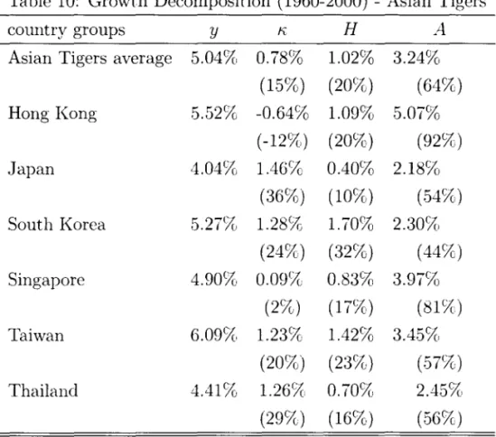
5.2 The Asian Tigers Growth Miracle
In Table 10 we present grovvth decomposition results for the Asian Tigers. This table
re-inforces our conclusion that growth miracles were mainly productivity miracles. \Vith the exception of South Korea, all countries in this group experienced a contribution of produc-tivity grmvth higher than 50%.:1O Productivity grmvth was particularly strong in Hong Kong
and Singapore, contributing for more than 80% of output per worker growth.
Table 10: Growth Decomposition (1960-2000) - Asian Tigers
country groups y K H A
Asian Tigers average 5.04% 0.78% 1.02% 3.24%
(15%) (20%) (64%)
Hong Kong .5.52% -0.64% 1.09% 50-o/c ' . I o
(-12%) (20%) (92%)
Japan 4.049() 1.46% 0.40% 2. 189()
(36%) (10%) (54%)
South Korea 5.27% 1.28% 1.70% 2.309(,
(24%) (32%) (44%)
Singapore 4.90% 0.09% 0.83% 3.97%
(2%) (17%) (81%)
Taiwan 6.09% 1.23% 1.42% 3.45%
(20%) (23%) (57%)
Thailand 4.41% 1.26% 0.70S{, 2.45%
(29%) (16%) (56%)
I\ote: The numbers in parenthesis are the relative contributions of each factor to output per worker growth.
30These reslllts confirlll the ones obtaineel bv Klenow anel Rodrigllez-Clare (1997) anel ma,\' seeIll at odds with the careful stuely by Young (1995), which showeel that the East Asian Tigers (Hong Kong. Singapore. Taiwan anel Korea) gre\,' mostly throllgh factor accunmlation. As pointed out b,\' Klenow anel Rodriguez-Clare. the differences are mainly ellle to the fact that Young eloes not attribute to procluctivit:, the growth in ph,\'sical capital induced by proelnctivit,\,. as wc anel Klenow anel Roelriguez-Clare do, For a more thorongh comparison of onr reslllts with YOllng (199.5), see Ferreira. Pessoa and VCl050 (2004),
Figure 6 below presents the evolution of A for the Asian Tigers and the region average. The figure shows that, as opposed to what occurred in Latin America, productivity continued to grow strongly after 1975.:n
セZZKiMᄋMMMMセMMMMセMMMMMMMMMMMMMMMMMMMMMMMMMMセセMMMMMMMM
160+---__ MMセMMセMMMMMMMMMMMMMMMMMMMMMMMMMMMMMQTPKMMMMMMMMMセセMMセセセMMMMMMMMMMMMMMMMセMMセセセ@
TPセ]ヲセセセセMMMMMMMMMMMMMMMMMMMMMMMMMMMMMMセMMMMMMMMMMMMMMM
.-:- Asian Tigcrs -- USA Taiwan J-Iong K()Tlg_= Korea -- Singaporc 1
Figure 6: Productivity of the East Asian Tigers, 1960-2000 (US, 1960=100)
6
Conclusions
This article presents a group of exercises on leveI and growth decomposition for a sample of countries from 1960 to 2000. The developrnent decompositions for earlier years reached conclusions that are quite diverse from those in the literature. Klenow and Rodriguez-Clare (1997), Prescott (1998), Hall and Joncs (1999) anel Easterly and Levine (2001). for instance, showed that the bulk of international output per worker dispersion is caused by total factor prodllctivity differences. These studies used 1985 or later data. \Ve showed that at least until 1975 factors of production, namely capital and education, " .. ere the main source of incorne eiispersion and that productivity variance was considerably srnaller than in late years. Only after 1975 the prominence of proeiuctivity started to show up in the data. The increase in the reI ative importance of productivity relative to factors is associated with the recluction across the perioei in the variance of factors due to convergence in the capital-output ratio anel the increase in proeluctivity variance in the nineties.
;HThis fact has also heen noticed by Collins anel Bosworth (1996) anel Rodrik (1999). )Jote. however. that for ali countries in this group. the marginal product of capital dedined throughout the period dul' to the sharp increase in the capital-olltpllt ratios. In 2000 the PjlyK of the East Asian Tigers was dose to that of the USo
The growth decomposition exercises showed that the reversal of the relative importance of productivity vis-a-vis factors is explained by the very good (bad) performance of productivity of fast (slow) growing countries in the period. Although most countries experienced capital deepening and improvements in education, exceptional growth performances were mostly due to productivity growth. Hence, although average growth in the period wa.';; mostly due to factors accumulation, its variance is explained by productivity.
The importance of productivity in explaining t he dispersion of output per worker reveals the dominance of country or region-specific factors in recent development experiences. The stagnation of Latin America, for instance, is mostly explained by a significant decline in productivity, while the Asian Tigers ":\iIiracle" is mostly a productivity miracle. Although we have now a number of ''TFP theories" (e.g., Parente and Prescott (2000), Acemoglu, Johnson and Rohinson (2001)) there are not many studies looking at its time series behavior - \vhen and why did '"A" in a particular economy changed its path - nor empirical studies linking TFP to exogenous variables. The results in the present study indicate that tllose may be very fruitful paths of research, given their importance to the understanding of development expenences.
From a theoretical standpoint, despite the importance of productivity in explaining tlle dispersion of the leveI and grcwvth rates of output per workeL the implication that the neoclassical growth rnodel is inconsistent with the development facts does not seerns to be warranted,:12 for three reasons. First, factors accurnulation account for the bulk of rnean grO\vth of output per worker between 1960 and 2000. Second, at least until 1975, factors were the main source of income disparity across countries. Third. at least until 1990, the increase in thc reIative irnportance of productivity was mainly due to thc reduction of factors variance (in particular, of the capital-output ratio), which is consistent with the cOllvergence mechanism predicted by the neoclassical grO\\ih rnodel. These results suggest that a ver-sion of the neoclassical growth model. suitably modified to take into account differcnces in productivity. may be a useful frarnework to interpret developrnent facts.;;:3
References
[1] Acemoglu, D., S. Johnson and J. Robinson, 2001. ''The Colonial Origins of Comparativc Developmcnt: An Ernpirical Investigation," Amer'ican Economic Review
91(5): 1369-1401.
ZIセfッイ@ a criticism along these lines. see Easterly aml Lc\'ine (2001).
3:30ne exarnple of this approach is Parente aml Prescott (1994). Recent papers pnrsuing this linl' of research incl mie Barelli and Pessôa (2002) allll Herrendorf and Teixeira (20m).
[2J Acemoglu, D., S. Johnson and J. Robinson, 2002 "Reversal of Fortune: Ge-ography and In.,>titution",> in the セQ。ォゥョァ@ of the セQP、・イョ@ World Incorne Distributions"
Quarterly Journal of Economics, 117: 1231-1294.
[3J Baier, S. L., G. P. Dwyer, Jr. and R. Tamura, 2004. "How Irnportant Are Capital
and Total Factor Productivity for Econornic Growth?," :\Iirneo, Research Departrnent, Federal Reserve Bank of Atlanta.
[4J
Barelli, P. and S. de Abreu Pessôa, 2002. "A rvIodel of Capital Accurnulation and Rent Seeking". vVorking Paper EPGE, n. 449.[5J Barro, R. and J. W. Lee, 2000. "International Data on Educational Attainrncnt: Updates and Irnplications," NBER \Vorking Paper #7911.
[6J Benhabib, J and M. Spiegel, 1994. " The Role of Hurnan Capital in Economic
Developrnent: Evidence from Agregate Cross-Country Data.", Journal of Alonetary
Economics, n. 34, pg 143-73.
[7J Bills, M. and P. Klenow, 2000. "Does Schooling Cause Growth?," American
Eco-nomic Review. 90(5): 1160-1183.
[8J Collins, Susan M. and B. P. Bosworth, 1996. :'Econornic GrO\vih in East Asia: Accumulation versus Assimilation," Brookings Papers on EcoTlomic Activity, 2: 135-203. [9J Easterly, W., 2001. "The Lost Decades: De\"€loping Countries' Stagnation in Spite
of Policy Reforrn 1980-1998," Journal of Economú: Growth, 6 (June): 135-157.
[lOJ
Easterly,W., N.
Loayza and P. Montiel, 1997. "Has Latin Arnerica's Post-Reform GrO\vih Been Disappointing?," Journal of InteT7wtional Economic8, 43: 287-311.[11J Easterly, W. and R. Levine, 2001. ,·It's not Factor Accurnulation: Stylizcd Facts
and GrO\vih セiッ、・ャウNGᄋ@ The World Bank Economic Reuiew, 15 (2): 177-219.
[12J Engerman, S. and K. Sokoloff, 1994. "Factor Endowments. Institutions, anel Dif-ferential Path of Growth Among New \Vorld Economies: A View From Economic: His-torians of the Unitcd States," NBER Historical Paper #66.
[13J Ferreira, P., Pessôa, S. and F. Veloso, 2004. 'The Tyranny of Numbers: Putting Young's TFP Numbers in \Vorld Perspectivc" (Provisory Title)
[14J
Fraumeni, B., 1997. 'The セi」。ウオイ・@ of Depreciation in thc US National Accounts,"Survey of Current Business. July.
[15J
Gollin, D., 2002. "Getting Income Shares Right: Self Employment, Unincorporated Entcrprise, and the Cobb-Douglas Hypothesis," Journal of Political Economy, 110(2):458-472.
[16J
Hall, R.E. and C. Jones, 1999. "\Vhy do Some Countries Produce so :\Iuch :Vlore Output per Worker than Others?," Quarlerly JouT1wl of Economics, February, 114:83-116.
[17J
Herrendorf, B. and A. Teixeira, 2003. "Monopoly Rights Can Reduce Income BigTime". lvIimeo.
[18J
Heston, A., R. Summers and B. Atten, 2002. Penn- World Table, version 6.1.Center for International Comparisons at the University of Pennsylvania.
[19J
King, R. G. and R. Levine, 1994. "Capital Fundamentalism, Economic Develop--ment, and Economic Grmvth," Carnegie-Rochester Conference Series on Public Policy,40: 259-292.
[20] Klenow, P. J. and A. Rodríguez-Clare, 1997. ''The Neoclassical Revival in Gro\\ih Economics: Has it Gone Too Far?" NBER AfacTOeconomics Annual 1997 eds. Ben S.
Bernanke and Julio J. Rotemberg, Cambridge, .\IA: The .\HT Press,
73-103.
[21] Lucas, R. E., Jr., 1990. "VV11Y Doesn't Capital Flow from Rich to Poor Countries?,"
Amerú:an Economic Review 80 (.\Iay): 92-96.
[22] Maddison, A., 1995. "lHonitoring the vVo7"ld Economy: 1820-1992." Paris: OECD.
[23] Mankiw, N. G., 1995. ''The Growth of NatiorL'3." Brooking Papers 077 Economic
Activity 1: 275-326.
[24] Mankiw, N. G., Romer, D. and D.Weil., 1992. "A Contribution To The Empirics Of Economic GrO\vth." Quarterly Journal of Economics 107 (.\Iay): 407-437.
[25] Mincer, J., 1974. Schooling, E:xpe7'ience. and Earnings, National Bureau ofEconomic
Research, distributed by Columbia University Press.
[26] North, D., 1990. Institutions, Insiitutional Change, and Economic Performance.
Cambridge University Press.
[27] Parente, S and E. Prescott, 1994 .. , Barriers to Technology Adoption and
Develop--rnent". JOUTnal of Political Econorny. 102 (2): 298-321.


![Figure 4: :\Iarginal Product of CapitaL Sclccted Country Groups (1960-2000)]](https://thumb-eu.123doks.com/thumbv2/123dok_br/15634186.109967/19.921.145.737.276.619/figure-iarginal-product-capital-sclccted-country-groups.webp)