GEOMETRIC QUALITY ASSESSMENT OF LIDAR DATA BASED ON SWATH
OVERLAP
A. Sampath *a, H. K. Heidemann b, G. L. Stensaas b aSGT, Contractor to US Geological Survey’s EROS Data Center
- (aparajithan.sampath.ctr)@usgs.gov b
US Geological Survey EROS Data Center – (kheidemann, stensaas)@usgs.gov
KEY WORDS: Lidar, Quality, Geometry, Relative, Accuracy
ABSTRACT:
This paper provides guidelines on quantifying the relative horizontal and vertical errors observed between conjugate features in the overlapping regions of lidar data. The quantification of these errors is important because their presence quantifies the geometric quality of the data. A data set can be said to have good geometric quality if measurements of identical features, regardless of their position or orientation, yield identical results. Good geometric quality indicates that the data are produced using sensor models that are working as they are mathematically designed, and data acquisition processes are not introducing any unforeseen distortion in the data. High geometric quality also leads to high geolocation accuracy of the data when the data acquisition process includes coupling the sensor with geopositioning systems. Current specifications (e.g. Heidemann 2014) do not provide adequate means to quantitatively measure these errors, even though they are required to be reported. Current accuracy measurement and reporting practices followed in the industry and as recommended by data specification documents also potentially underestimate the inter-swath errors, including the presence of systematic errors in lidar data. Hence they pose a risk to the user in terms of data acceptance (i.e. a higher potential for Type II error indicating risk of accepting potentially unsuitable data). For example, if the overlap area is too small or if the sampled locations are close to the center of overlap, or if the errors are sampled in flat regions when there are residual pitch errors in the data, the resultant Root Mean Square Differences (RMSD) can still be small. To avoid this, the following are suggested to be used as criteria for defining the inter-swath quality of data:
a) Median Discrepancy Angle
b) Mean and RMSD of Horizontal Errors using DQM measured on sloping surfaces
c) RMSD for sampled locations from flat areas (defined as areas with less than 5 degrees of slope)
It is suggested that 4000-5000 points are uniformly sampled in the overlapping regions of the point cloud, and depending on the surface roughness, to measure the discrepancy between swaths. Care must be taken to sample only areas of single return points only. Point-to-Plane distance based data quality measures are determined for each sample point. These measurements are used to determine the above mentioned parameters. This paper details the measurements and analysis of measurements required to determine these metrics, i.e. Discrepancy Angle, Mean and RMSD of errors in flat regions and horizontal errors obtained using measurements extracted from sloping regions (slope greater than 10 degrees). The research is a result of an ad-hoc joint working group of the US Geological Survey and the American Society for Photogrammetry and Remote Sensing (ASPRS) Airborne Lidar Committee.
* Corresponding author
1. INTRODUCTION
1.1 Lidar data geometric assessment
Lidar data, particularly for larger area projects, are usually collected in long swaths. These swaths often overlap for a variety of reasons, including providing higher point density, assurance of coverage, calibration, etc. These overlapping regions of the data sets provide the user of the data with an opportunity to test the geometric quality of the data. As in Latypov, 2002, we are more concerned with providing a method of quantifying the relative accuracy of point cloud by making measurements between the points in the overlapping regions. In this paper, we do not talk about “correcting” the data either by adjustment of calibration parameters (Habib et al., 2010) or by the practice of strip adjustment (e.g., Munjy 2015). Latypov analyses the vertical differences between conjugate surface patches in the overlapping regions of the point cloud as a function of surface density and flatness. Other researchers (Habib et al., 2010; Sande et al., 2010) use planar features to
assess the relative accuracy and also to adjust the overlapping strips to minimize the point to plane distance. In this paper, we describe the efforts of a collaborative effort between the US Geological Survey and the American Society for Photogrammetry and Remote Sensing (ASPRS) to establish guidelines on Quality Assurance and Control (QA/QC) of lidar data. We present methods to quantify the quality of lidar data in terms of their relative vertical, horizontal accuracy, and also quantify the systematic errors present in lidar data.
1.2 Scope of the paper
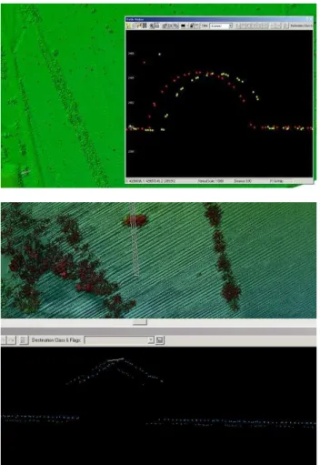
Figure 1 shows errors found in swath data, indicating inadequate quality of calibration. The images show profiles of objects in overlapping regions of adjacent swaths. It is the goal of this research to have methods that automatically flag overlapping swaths that have these errors. Such errors indicate poor geometric data quality, and are often the result of inadequately rigorous calibration (system or boresight) procedures.
Calibration should be performed as directed by the instrument manufacturer either periodically, or based on usage. Calibration should also be performed when an instrument has had a shock or vibration (which potentially may put it out of calibration) or whenever observations appear questionable. In many cases calibration can be performed in situ (field tests or self-calibration), and it is a standard practice among Lidar data providers to perform such a calibration. However, there is no single/accepted method of lidar system calibration, and this can lead to varying quality of data, depending on the validity and efficiency of calibration procedure. It is also recognized that lidar systems are unique, and each type may have different sensor models that demand different calibration philosophies. It is not the goal of this document to discuss calibration procedures for the instruments, but to discuss processes to test the quality of calibration.
Quality Control (QC) is used to denote post-mission procedures for evaluating the quality of the final Lidar data product (Habib et al., 2010). The user of the data is more concerned with the final product quality, than the system level Quality Assurance procedures that may vary depending on the type of instrument in use. Thus, as far as the user is concerned, the acquisition system is a black box. The user wants to avoid situations as shown in Figure 1, without having to understand the entire data acquisition process and sensor models.
Figure 1. Errors found in swath data indicating inadequate quality of calibration. The images show profiles of objects in
overlapping regions of adjacent swaths
The QC procedures discussed in this paper are system agnostic and work with only point cloud data delivered by the data provider. The procedures use three concepts to quantify the inter-swath quality of lidar data.
Median Discrepancy Angle
Mean and Root Mean Square
Differences(RMSD) of Horizontal Errors
Mean and RMSD of vertical errors
These three quantities can provide a more complete understanding of the quality of lidar system calibration and data acquisition.
2. THE INTER SWATH DATA QUALITY METRICS (DQM)
2.1 DQM Definitions
Calibration methods can be different for different sensors, and will change as new types of sensors are introduced in the future. This further increases the need to have standard processes to test the quality of calibration. The quality of calibration can be judged by observing the area covered by overlapping Lidar scans. Any quantitative measures on the quality of calibration can be generated by analyzing these regions. For government procurement guidelines, it is desired to have a measure of mis-registration between overlapping scans/point clouds, after they have been calibrated and before further processing (i.e. point cloud classification, feature extraction, etc.) is done. This measure can also be seen as Data Quality Measure (DQM). Many researchers (Habib et al. 2010; Latypov 2002; Sande 2010) have discussed methods of reporting registration errors between adjacent strips of Lidar data. The registration errors can be treated as indicators of the quality of calibration. The importance of correct calibration of a lidar system to the data acquisition process and to the geometric quality of data cannot be overstated. A good calibration involves precise measurements between the various subsystems of lidar system, including the lidar sensor/instrument, GPS receiver and Inertial Measurement Units (IMU).
Figure 2 shows a profile of a surface that falls in the overlapping region of two adjacent swaths. The surface as defined by the swaths is shown in dotted lines while the solid profile represents the actual surface. A poorly calibrated system leads to at least two kinds of errors in lidar data. The first one is that the same surface is defined in two (slightly) different ways (relative or internal error) by different swaths, and the second one is the deviation from actual surface (absolute error). For most users of lidar data, the calibration procedures are of less concern than the data itself. However, they would like to have a process to test the quality of calibration of the instrument, because a well calibrated instrument is a necessary condition for high quality data. While data providers make every effort to reduce the kind of errors shown in Figure 1 and 2, there are no standard methodologies in current QC processes to measure the internal goodness of fit between adjacent swaths (i.e. internal or relative accuracy).
Absolute error
Relative horizontal
error: not accounted for currently
Relative vertical error
Swath # 1
Swath # 2
Figure 2 Surface uncertainties in hypothetical adjacent swaths. Profile of nominal surface is shown as solid line while the surface defined by swath # 1 and swath # 2 are shown as dotted
lines
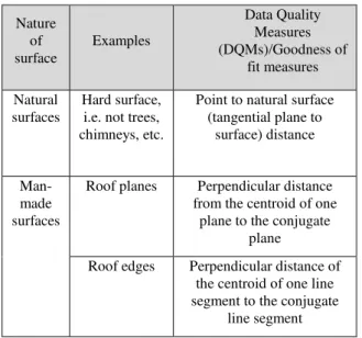
Current specifications documents (e.g. Heidemann 2014) do not provide adequate guidance on measuring the inter-swath (internal accuracy) goodness of fit of lidar data. Three quantities that measure the inter-swath goodness of fit are listed in Table 1. These measures describe the discrepancy between two overlapping point clouds and are often used to obtain optimal values of the transformation parameters. The DQMs are not direct point-to-point comparisons because it is nearly impossible for a lidar system to collect conjugate points in different swaths. It is easier to identify and extract conjugate surfaces and related features (e.g. roof edges) from lidar. The DQMs over natural surfaces and over roof planes assume that these conjugate surfaces are planar, and determine the measure of separation between a point and the surface (plane). The DQM over roof edges extract break lines or roof edges from two intersecting planes and measure their discrepancy.
Nature of surface
Examples
Data Quality Measures (DQMs)/Goodness of
fit measures
Natural surfaces
Hard surface, i.e. not trees, chimneys, etc.
Point to natural surface (tangential plane to
surface) distance
Man-made surfaces
Roof planes Perpendicular distance from the centroid of one
plane to the conjugate plane
Roof edges Perpendicular distance of the centroid of one line segment to the conjugate
line segment
Table 1 Data Quality Measures (DQMs) or inter-swath goodness of fit measures
The DQM over natural surfaces based point to (tangential) plane distance is the most easy to implement as it does not involve feature extraction. It is also easy to find enough of these planar features in a uniform sampling of the overlapping regions of the point cloud, by defining planar regions as those with small standard deviations of plane fit.
This measure is calculated by selecting a point from one swath
(say point ‘p’ in swath # 1), and determining the neighboring points (at least three) for the same coordinates in swath # 2.
Ideally, the point ‘p’ (from swath # 1) should lie on the surface
defined by the points selected from swath # 2. Therefore, any departure from this ideal situation will provide a measure of discrepancy, and hence can be used as a DQM. This departure is measured by fitting a plane to the points selected from swath # 2, and measuring the (perpendicular) distance of point ‘p’ to this plane. As shall be made clear, the point-to-plane DQM along with the information about the normal vector (i.e. the
distance “vector”) is very important in describing the errors in
the overlapping regions of the point cloud.
Point to (tangential) plane distance
Point p in swath # 1
Tangential plane Surface described by
points in swath # 2
Figure 3 Representation of DQM over natural surfaces. Point
‘p’ (red dot) is from swath # 1 and the blue dots are from swath
# 2
2.2 DQM implementation
The US Geological Survey (USGS) has prototyped software that implements the concept of point to plane DQM over natural surfaces. The prototype works on ASPRS’s LAS format files containing swath data. If the swaths are termed Swath # 1 and Swath # 2 (Figure 4), the software uniformly samples single
return points in swath # 1 and chooses ‘n’ (user input) points. The neighbors of these ‘n’ points (single return points) in swath
# 2 are determined.
Figure 4 Implementation of prototype software for DQM analysis
In the prototype software, there are three options available for determining neighbors: Nearest neighbors, Voronoi neighbors or Voronoi-Voronoi neighbors. However, other nearest
neighbor methods such as “all neighbors within 3 m” are also
acceptable. A least squares plane is fit through the neighboring points using eigen value/eigen vector analysis (in a manner similar to Principal Component Analysis). The equation of the plane is the same as the component corresponding to the least of the principal components. The eigenvalue/eigenvector analysis provides us the planar equations as well as the root mean square error (RMSE) of the plane fit. The use of single return points in conjunction with a low threshold for RMSE is used to eliminate sample measurements from non-hard surfaces (such as trees, etc.). The DQM software calculates the offset of the point (say
‘p’) in Swath # 1 to the least squares plane. The output includes
the offset distance, as well as the slope and aspect of the surface (implied in the planar parameters).
The advantages of using the method of eigenvalues/PCA/least squares plane fit are fivefold:
a) The RMSE of plane fit provides an indication of the quality of the control surface. A smaller eigenvalue ratio indicates high planarity and low curvature. It provides a quantitative means of measuring control surfaces.
b) It is the accepted “point cloud” technique, and has been developed on the back of a rich technical literature.
c) Converting surfaces to raster results in (however small) loss of accuracy that is not easily quantified. It also introduces another level of processing that introduces products not used anywhere else. d) The arc cosine of Z component of eigenvector gives
the slope of terrain
e) The normal vector of the planes are crucial to calculate the horizontal errors
3. QUANTIFYING ERRORS
3.1 Vertical and Systematic Errors
The DQM measurements need to be analyzed to extract estimates of horizontal and vertical error. To understand these errors associated with overlapping swaths, the DQM prototype software was tested on several data sets, as well as against datasets with known boresight errors. The output of the prototype software not only records the errors, but also the x, y and z coordinates of the test locations, eigenvalues and the eigenvectors, as well as the least squares plane parameters.
The analysis mainly consists of three parts
a) The sampled locations are categorized as functions of slope of terrain: Flat terrain (defined as those with slopes less than 5 degrees) versus slopes greater than 10 degrees.
b) For estimates of relative vertical error, DQM measurements from flat areas ( slope < 5 degrees) are identified:
DQM errors are measured as a function of distance of sample check points from center of overlap (Dco). The center of overlap is defined as line along the length of the overlap region passing through median of sample check points (Figure 5)
The Discrepancy Angle (dSi) (Illustrated in Figure 5) at each sampled location, defined as the arctangent of DQM error divided by Dco, is measured
c) The errors along higher slopes are used to determine the relative horizontal errors in the data as described in the next section.
Profile view: Discrepancy Angle s=arc tangent (dSi/Dco)
dsi
dsj
Center of overlap
Figure 5 Analysis of DQM errors and center line of overlap
It must be noted that the possibility of outliers cannot be ruled out. To avoid these measurements, an outlier removal process using robust statistics was used. For each category (Flat and higher slopes separately), the following quantities were calculated:
Only those points that are deemed acceptable are used for further analyses. The Median Absolute Deviation method is only one of many outlier detection methods that can be used. Any other well defined method should also be an acceptable method.
Relative vertical errors are easily estimated and defined as DQM measurements made on locations where the slope is less than 5 degrees. Figure 6 shows two plots of DQM output from flat areas as function of the distance from the centerline of swath overlap. The analysis of errors based on point-to-plane DQM can use the sign of the errors. If the plane (least squares
plane) in swath #2 is “above” the point in swath # 1, the error is
considered positive, and vice versa. Both these methods of representation of errors can be used to easily identify and interpret the existence of systematic errors also.
Figure 6 Visual representations of systematic errors in the swath data. The plots show DQM errors isolated from flat regions (slope < 5 degrees). 6(a) plots signed DQM Errors vs. Distance
from the center of Overlap, while 6(b) plots Unsigned DQM errors vs. Distance from center of overlap.
In the presence of substantial systematic errors, relative vertical errors tend to increase as the measurements are made away from the center of overlap. In particular, errors that manifest as roll errors (the actual cause of errors may be completely different) will cause a horizontal and vertical error/discrepancy in lidar data. Therefore it is possible to observe these errors in the flat regions (slope less than 5 degrees), as well as sloping regions. In the flat regions, the magnitude of vertical bias increases from the center of the overlap. Using the sign conventions for errors defined previously, these errors can be modelled as straight line passing through the center of the overlap (where they are minimal).
In Figure 7, the red dots are measurements taken from flat regions (defined as those with less than 2 degrees), the green and the blue dots are taken from regions with greater than 20 degrees slope. The green dots are measurements made on slopes that face away from the centerline (perpendicular to flying direction), whereas the blue dots are measurements taken on slopes that face along (or opposite to) the direction of flight.
If non-flat regions that slope away from the centerline of overlap are available for DQM sampling, horizontal errors can also be observed. The magnitude of horizontal errors is usually greater than that of the vertical errors, for the same error in calibration. This is also reflected in the plots shown in Figure 7.
Figure 7 DQM errors as function of distance of points from center of the overlap (each column has different scales). The blue line is a regression fit on the error as function of distance
from center of overlap
In Figure 7, the first column shows the plot of DQM versus distance of sample measurements from centerline of overlap. The consistent and quantifiable slope of the red dots indicates that Roll errors are present in the data. A regression line is fitted on the errors as a function of the distance of overlap. The slope of the regression line defined by the red dots is termed
‘Calibration Quality Line’ (CQL). The slope of the CQL corresponds theoretically to the mean of the all the Discrepancy Angles measured at each DQM sample test points. In practice, the value is closer to the median of the measured Discrepancy Angles (perhaps indicating outliers).
Pitch errors cause discrepancy of data in the planimetric coordinates only, and the direction of discrepancy is along the direction of flight. The discrepancy usually manifests as a constant shift in features (if the terrain is not very steep). This requires them to be quantified using measurements made from non-flat/sloping regions. Figure 7 shows that this can be achieved (blue dots in the second column indicate pitch errors) using the DQM measurements. The blue dots indicate that there is a constant shift along the direction of flight. The presence of red dots close to the zero error line (and following a flat distribution) indicates that these errors are not measurable in flat areas. The presence of green dots closer to the zero line also indicates that pitch errors are not measurable in slopes that face away from the flight direction. The third column in Figure 7 indicates that when these errors are combined (as is almost always the case), it is possible to discern their effects using measurements of DQM on flat and sloping surfaces.
3.2 Horizontal Errors
The process of measuring the point-to-plane DQM also provides us with estimates of the normal vectors of the planar region, along with an estimate of curvature. It will be shown in the section below that if the neighborhood is large enough (this ensures that the planar fit is stable), and if the curvature is low, the normal vectors, and the point-to-plane DQM can be combined to estimate the presence of relative horizontal errors in the data. Many researchers have identified, extracted and compared the position of conjugate man-made features to estimate horizontal errors in the data. However, if the objective The International Archives of the Photogrammetry, Remote Sensing and Spatial Information Sciences, Volume XLI-B1, 2016
is to obtain summary statistics of horizontal errors (i.e. the mean, standard deviation and the root mean square deviation), it can be shown that estimates can be obtained without performing feature extraction.
Figure 8 Three points the measured DQMs, the corresponding planar patches (PL1, PL2, PL3) in Swath #1(green) and Swath # 2 (blue) and their virtual point of
intersection (P’ and P) are shown
Consider any three points that have been sampled for measuring
DQMs in Swath # 1 ( ,
in Figure 8). Let these points be selected from areas that have higher slopes. These three points have corresponding neighboring points and three planar patches measured in Swath
# 2. Let’s assume that these three planar patches intersect at
point P in Swath # 1(a virtual point, point P may not exist
physically). Let’s assume that the conjugate planar patches in Swath # 2 intersect at P’. Let the equations (together called Equation 1) of the three planes be
(1)
If are the direction cosines of the normal vectors of the planar patches, then is the signed perpendicular distance of the planes from the origin.
If the intersection point P is represented by
then Equation 1 can be written as: . Similarly, for
the point P’ in Swath # 2, we have .
If , and we
get
(2)
Expanding Equation 3, we get:
However , therefore we get
(3)
Since we are interested only in , and there are no changes to the normal vectors or displacement vectors when there is a pure shift involved, the analysis can be further simplified by shifting the origin to (i.e. . Therefore Equation 3 becomes
(4) Since we are measuring the discrepancy in calibrated point clouds, the expectation is that are small, and hence the product can be neglected, (typically, . Therefore Equation 4 becomes:
(5) Equation 5 is the equation of planes intersecting at , and at a signed perpendicular distance from the origin. Since the origin (the point P) lies on all three planar patches, and again emphasizing the fact that we are testing calibrated data, values will be very close to the three measured point to plane distance errors or DQMs. This is because the point to perpendicular plane distance does not change if the point P and p1 lie on the same plane, and the planes (PL1 in Swath #1 and Swath #2) are near parallel. Therefore Equation 6 can be approximated by
(6)
Considering the same analysis for all triplets of points of patches with higher slopes, we replace with , with N (which is a matrix containing normal vectors
associated all ‘n’ DQM measurements that have higher slopes),
and as the vector of all DQM measurements. This leads to the simple least squares equation for
(7) is easily calculated and the standard deviation for is also easily obtained by using standard error propagation techniques.
The methodology to estimate provides quantitative estimate of the mean relative horizontal and vertical shift/displacement of features in the inter swath regions of the data. Assuming pure shifts is not unreasonable because the point clouds are nominally calibrated and traditionally, geospatial data have been assessed in terms of mean/bias, standard deviation and root mean square deviation. Mean/bias reduces the error in geospatial data to a shift, and standard deviation is used to explain the departure from this assumption. In the theory described above, the same assumptions have been made. The three dimensional errors are also described as a shift (Mean), and the departure (standard deviation) from this assumption.
4. IMPLEMENTATION ANALYSIS AND CONCLUSION
4.1 Implementation and Analysis
The DQM point-to-plane natural surfaces algorithm was used to test several data sets with the US Geological Survey. The software implementation was used on complete data sets, and not just on a few swaths. The results were summarized in an excel sheet, a sample of which is shown in Figure 9. The output summarizes the vertical, and the horizontal error (mean, standard deviation and RMSD) for each pair of overlapping swaths in a project.
Figure 9. A sample excel sheet showing the summarizing of the results. The excel sheet shows the vertical, horizontal errors, systematic errors present between all overlapping swaths in a
complete project.
Most users and owners of data will not look at swath data directly. Most of the processing, analysis and conflation with other geospatial data is performed with data in tiles. The summary of the analysis shown in excel sheet provides a way to directly look at those swath pairs that indicate higher errors. The implementation does not call for any feature extraction of planar features. It uses only regions that are sampled and are highly planar, based on the standard deviation of the plane fit. The analyses have been used to identify errors in urban, semi urban and other areas with no man made features (but with higher slopes). It is sufficient to have reasonably planar regions that have high slopes than actual man made planar surfaces.
4.2 Conclusion
Current accuracy measurement and reporting practices followed in the industry and as recommended by data specification documents (e.g. Heidemann 2014) potentially underestimate the inter-swath errors, including the presence of systematic errors in lidar data. Hence they pose a risk to the user in terms of data acceptance (i.e. a higher potential for Type II error indicating risk of accepting potentially unsuitable data). For example, if the overlap area is too small or if the sampled locations are close to the center of overlap, or if the errors are sampled in flat regions when there are residual pitch errors in the data, the resultant Root Mean Square Differences (RMSD) can still be small. To avoid this, the following are suggested to be used as criteria for defining the inter-swath quality of data:
a) Median Discrepancy Angle
b) Mean and RMSD of Horizontal Errors using DQM measured on sloping surfaces
c) RMSD for sampled locations from flat areas (defined as areas with less than 5 degrees of slope)
4000-5000 points are uniformly sampled in the overlapping regions of the point cloud, and depending on the surface roughness, to measure the discrepancy between swaths. Care must be taken to sample only areas of single return points only.
Point-to-Plane data quality measures are determined for each sample point. These measurements are used to determine the above mentioned quality metrics. This document details the measurements and analysis of measurements required to determine these metrics, i.e. Discrepancy Angle, Mean and RMSD of errors in flat regions and horizontal errors obtained using measurements extracted from sloping regions (slope greater than 10 degrees).
ACKNOWLEDGEMENTS
The authors would like to acknowledge the contributions and support of the members of the ASPRS and the US Geological
Survey’s National Geospatial Technical Operations Center
(NGTOC) for this work.
REFERENCES
Habib, A., Kersting, A P., Bang, K I., and Lee, D C., 2010. Alternative Methodologies for the Internal Quality Control of Parallel LiDAR Strips. IEEE Transactions on Geoscience and Remote Sensing, vol. 48, no. 1, pp. 221-236, Jan. 2010. doi: 10.1109/TGRS.2009.2026424
Heidemann, H. K., 2014. Lidar base specification version 1.2, U.S. Geological Survey Techniques and Methods, Book 11, Chapter. B4, 63 p
.
Latypov, D., 2002. Estimating relative LiDAR accuracy information from overlapping flight lines. ISPRS Journal of Photogrammetry and Remote Sensing, 56 (4), 236–245.
Munjy, R., 2014. Simultaneous Adjustment of LIDAR Strips. Journal of Surveying Engineering 141.1 (2014): 04014012.
Sande, C., Soudarissanane, S., Khoshelham, K.,2010. Assessment of Relative Accuracy of AHN-2 Laser Scanning Data Using Planar Features. Sensors . 10, 8198-8214. The International Archives of the Photogrammetry, Remote Sensing and Spatial Information Sciences, Volume XLI-B1, 2016