NBER WORKING PAPER SERIES
BRIGHT MINDS, BIG RENT:
GENTRIFICATION AND THE RISING RETURNS TO SKILL
Lena Edlund
Cecilia Machado
Michaela Sviatchi
Working Paper 21729
http://www.nber.org/papers/w21729
NATIONAL BUREAU OF ECONOMIC RESEARCH
1050 Massachusetts Avenue
Cambridge, MA 02138
November 2015
We have benefitted from discussions with Joe Altonji, V. V. Chari, David Deming, Jonathan Fisher,
Jonathan Heathcote, Matthew Kahn, Shirley Liu, Douglas Lucius, Chris Mayer, Enrico Moretti, Marcelo
Moreira, Bernard Salanie, Aloysius Siow, Seminar participants at the Minneapolis Federal Reserve,
the Barcelona Graduate Summer School 2015, The Econometric Society World Congress August 2015.
We thank the New York Federal Statistical Research Data Centers, Baruch, Center for Economic Studies,
U.S. Census Bureau. Any opinions and conclusions expressed herein are those of the authors and do
not necessarily represent the views of the U.S. Census Bureau. All results have been reviewed to ensure
that no confidential information is disclosed. The views expressed herein are those of the authors and
do not necessarily reflect the views of the National Bureau of Economic Research.
NBER working papers are circulated for discussion and comment purposes. They have not been
peer-reviewed or been subject to the review by the NBER Board of Directors that accompanies official
NBER publications.
Bright Minds, Big Rent: Gentrification and the Rising Returns to Skill
Lena Edlund, Cecilia Machado, and Michaela Sviatchi
NBER Working Paper No. 21729
November 2015
JEL No. R21,R30
ABSTRACT
In 1980, housing prices in the main US cities rose with distance to the city center. By 2010, that relationship
had reversed. We propose that this development can be traced to greater labor supply of high-income
households through reduced tolerance for commuting. In a tract-level data set covering the 27 largest
US cities, years 1980-2010, we employ a city-level Bartik demand shifter for skilled labor and find
support for our hypothesis: full-time skilled workers favor proximity to the city center and their increased
presence can account for the observed price changes, notably the rising price premium commanded
by centrality.
Lena Edlund
Department of Economics
Columbia University
1002A IAB, MC 3308
420 West 118th Street
New York, NY 10027
and NBER
[email protected]
Cecilia Machado
Getulio Vargas Foundation (EPGE-FGV)
[email protected]
I know things will get better
You’ll find work and I’ll get promoted
We’ll move out of the shelter
Buy a bigger house and live in the suburbs
Tracy Chapman, Fast Car, 1988
The truth is that we are living at a moment in which the massive outward
migration of the affluent that characterized the second half of the twentieth
is coming to an end.
Ehrenhalt, The Great Inversion, 2013
1
Introduction
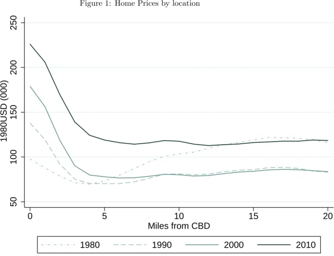
In 1980, US central-city residential real estate carried only a slight price premium.
In fact, prices were higher beyond than within 10 miles of city centers. Fast forward
20 years and the center commands the highest prices, whence they fall sharply with
distance for the first five miles and then flat lines. This pattern remains in 2010,
unscathed by the 2007 housing market correction (Figure 1).
What lies behind this urban renewal, or “gentrification”? The literature has noted
a number of signature features, such as depressed initial prices; and proximity to mass
transportation and amenities [Kahn, 2007, Glaeser et al., 2008, 2012, Guerrieri et al.,
2013].
Remains the question why centrality has increasingly come to bethe local amenity.
Gyourko et al. [2013] tied gentrification to a growing number of high-income households
combined with inelastic housing supply, the case in city centers by necessity but also
elsewhere courtesy of ordinances and the like [Ortalo-Magne and Prat, 2014]. However,
the US economy grew at a healthy clip throughout the 1950s and 1960s, a time of
urban decline and expansion of the suburbs [Jackson, 1985]. Granted, income growth
their share of income since the early-1950s and the top 1 percent since the mid-1960s
[Kopczuk et al., 2008, figure 2B].
The premium on central location seems to reflect more than a filling-up of scarce
space by high-income households. City-dwellers that ten, twenty years ago would have
headed straight for the suburbs at the first sign of baby now stay put despite cramped
living and high rents.1
This paper proposes that the roots of gentrification can be found in the shrinking
leisure of high-income households. This time scarcity, we hypothesize, has propelled
centrality to the top of the local amenities list.
Between 1965 and 2005, leisure grew but not for the college educated. In the
1985-2005 period, the contraction in leisure among college men was substantial enough
to result in an overall reduction for men (leisure grew among non-college men); for
women, leisure contracted across the board but at the twice the rate for college women
compared to non-college women [Aguiar and Hurst, 2009, table 2-2].
Aguiar and Hurst [2007, 2009] identified rising labor supply of the skilled to lie at
the core of this development. Census data bear this out. The fraction college graduates
who worked full time started to rise in the 1970s after three decades of barely moving,
Figures 2 and 3. Unsurprisingly, the increase was more pronounced for women. Since
1990, there has also been a notable increase in the fraction (men and women) working
50+ hours per week (or “long hours” to use the terminology of Kuhn and Lozano
[2006]).2
Long hours render non-work time scarce, planting low-utility activities such as
commuting in the cross-hairs. One of the simplest ways to control commuting is to
live close to work, which for skilled workers may mean the city center. There, by
definition, land is scarce and higher demand translates into higher land rents. In time,
local amenities adjust, boosting the attractiveness of the locality, further fueling the
gentrification process. The core driver, however, we propose, can be found in the labor
1
The October 23 2015New York Timesarticle “Growing Families That Stay Put” perhaps ironically gave “children” as the reasons for why New York City families choose to not move out of cramped apartments.
2
market processes that have produced a corps of high-income-low-leisure individuals
who live as singles or through assortative matching form dual-earner households.
Greater labor supply of the skilled is plausibly related to rising returns to skill [Katz
and Murphy, 1992, Juhn et al., 1993, Autor et al., 2008], a development linked to the
arrival of microprocessors in the early 1970s [Greenwood and Jovanovic, 1999, Hobijn
and Jovanovic, 2001]. The ensuing Information Technology Revolution has been a boon
to skilled employment growth in cities that were initially skilled [Berry and Glaeser,
2005, Moretti, 2013], a path dependency consistent with rapid technological change
[Beaudry et al., 2010].
Like a number of recent papers, e.g., Diamond [Forthcoming], Moretti [2013], we
will use college-employment demand shifters in combination with the 1970 city-level
industry structure to generate an arguably exogenous, city-level, skilled labor demand
shifter. The so called Bartik demand shifter helps us isolate our proposed labor-market
driven explanation from alternative explanations. For instance, high-income households
may always have valued central city living but in the past they were deterred by racial
antagonism or high crime [Glaeser et al., 2001]. Another possibility is reverse causality,
higher rents prod households to supply more labor [Johnson, 2012]).
Our hypothesis concerns the within-city distance-gradient of housing prices and
our empirical analysis will be performed at the tract level. To create create tract-level
variation we interact the city-level Bartik measure with the tract’s (population weighted
centroid) distance to the city center. In other words, we allow the city-specific demand
growth to propagate differentially according to the tract’s distance to the center.
Our main data set is a tract-level data set constructed from restricted-use US Census
micro-data covering the period 1980-2010. We use tract geocodes to calculate (centroid)
distance to a point in the central business district, and we will refer to this point as the
CBD. Geographically, we limit our sample to cities that were in the top-20 (population
wise) either in 1970 or 2010. There were 27 such cities3
which for simplicity we will
refer to as “top-20.” We include tracts within 35 miles of the CBD regardless of whether
3
they were in the same same city (or state) as the CBD. For the purpose of this paper,
the terms cities or metropolitan areas will be used interchangeably to refer to these
geographic entities.
To capture the rise of the high-income-low-leisure demographic, we focus on
full-time workers with a college degree among ages 25 to 55. This age group was chosen to
capture prime working ages, the years after college completion but before retirement
concerns. These ages are also key home buying ages.4
Throughout, we will control for a battery of fixed effects. Our preferred
specifi-cation has city-year fixed effects and city-specific distance controls. City-year fixed
effects absorbs any city-wide changes, including city-level labor demand shifts or credit
expansion (for a recent paper on the role of the latter, see Favara and Imbs [2015]).
City-specific distance controls stand in for tract fixed effects (but we will see that our
findings hold in a constructed tract panel data set that allows for tract fixed effects).
Allowing the Bartik demand shifter to have a differential impact on tracts 0-3 miles,
3-10 miles, 10-20 miles or 20-35 miles from the CBD we find the effect to be concentrated
near the center: almost three times stronger in the 0-3 mile core compared to the
contiguous 3-10 mile ring and almost seven times stronger than in the more distant
10-20 mile ring (the 20-35 mile ring served as the reference area). The implied price
changes from the reduced form estimates replicate very closely the actual level and
distance gradient of housing price increases.
First stage regressions reveal a strong relationship between full-time skilled workers
and the Bartik demand shifter. The relationship is strongest close to the CBD, and
then attenuates, the exact shape of the decline varying somewhat with the set of fixed
effects.
Turning to the relationship between full-time skilled workers and housing prices,
we find empirical support both in OLS regression analysis and in instrumented results
using the Bartik demand shifters. Full-time skilled workers not only chose to locate
close to the CBD, their presence there has a positive impact on prices. The implied
price changes from the IV analysis suggest that the growth of full-time skilled workers
can capture the 1980-2010 housing price changes (Figures 11-12).
4
Some of the cities with the steepest price increases have also seen the largest declines
in crime, New York City being a case in point with crime levels down by two-thirds
from their late-1980s levels. To investigate the role of improved public safety, we
split our cities into two equal sized groups, one with cities that saw large declines in
crime and one with cities that saw modest declines or increases over the 1985-2012
period.5
Qualitatively, results hold in both groups. Quantitatively, the effects were
also similar when fulltime was measured at 50 hours, but at the weaker measure of 40
hours, the high-decline cities saw a stronger effect than the low-decline cities. As a last
robustness check, we cross walk tracts to create a tract-level panel data set, allowing us
to include tract fixed effects, an inclusion that yields results similar to those obtained
using city-distance fixed effects. Further, we split tracts according to their percent
black population in 1980 (above or below the 1980 median) and find results to be
similar in the two samples, suggesting that the found results are not predicated on a
particular racial composition.
Finally, Census data allow us check our premise that skilled jobs are
disproportion-ately located in the central city, and we confirm this to be the case. Unskilled jobs,
on the other hand, are more dispersed and increasingly so. As a corollary, we expect
commuting time, especially for the skilled, to increase with residence distance to the
central city. We find that to be the case for men throughout the studied period and
increasingly also for women, consistent with the latter’s greater labor force attachment.
The remainder of the paper is organized as follows. Section 2 gives further
back-ground and literature review. Section 3 describes our empirical strategy and data set.
Section 4 presents the descriptives and results. Section 5 concludes.
2
Background and Existing Literature
This paper’s hypothesis turns on the increasing hours worked by high-income
house-holds, which, to paraphrase Ehrenhalt [2013], has given rise to an affluent class who
treat leisure as their most prized commodity.
5
Individual v. Household Labor Supply We have chosen to focus on individual
rather than household labor supply. Obviously, labor supply is a household decision.
However, the trends in household formation and labor supply behavior mean that the
distinction between individual and household labor supply behavior is fading.
First, there are more single headed households also among the skilled. While the
skilled tend to marry, they do so later. The median age of first marriage among college
educated was 28 in 2008, up from 23 in 1970; an additional five cohorts of college
educated singles.6
Second, among couples, the cross-wage elasticity of women’s labor supply is
shrink-ing [Heim, 2007]. That is, married women are increasshrink-ingly behavshrink-ing as if they were
single. Later marriage and higher risk of divorce [Edlund and Pande, 2002, Fernndez
and Wong, 2014] have reduced the economic value of marriage to women pushing women
into the labor force. Rising returns to skill figure prominently among pull factors.
As skilled women have become more attractive on the labor market, their currency
on the marriage market has also appreciated, at least that is one reading of the greater
degree of positive assortative mating evident in US data [Greenwood et al., 2014].
Positive assortative mating can boost married women’s labor supply since the women
who can most afford to stay home are also the ones leaving the most money on the
table.
In other words, the increase in women’s labor supply is mainly driven by
mar-ried women, e.g., Juhn and Murphy [1997], DiCecio et al. [2008], McGrattan and
Rogerson [2008], Schwartz [2010]. Married women’s working has given rise to more
dual-earner households. Although high-income dual-earner households are part of the
demographic change we hypothesize have fed gentrification, the rise in high-income
dual-earner households is one that is captured by the rise in skilled individuals’ labor
supply. High-income dual-earner households have interesting implications for the types
of apartments in demand (larger) and amenities sought after (family friendly?) and
thus bears on urban development. However, as far as housing prices are concerned,
their impact may be captured by individual-level measures of labor supply.
6
Drive ’Til You Qualify Our paper is in the spirit of what Mieszkowski and Mills
[1993] called the “natural evolution theory of urban development” augmented with
la-bor supply and household commuting decisions [White, 1977, Madden and White, 1980,
Madden, 1980]. Rappaport [2014] explicitly considered utility from leisure, thereby
sharpening the attention on commuting time. Empirically, his study made the case
for the relevance of the monocentric city model for mid-sized US cities, focusing on
Portland, Oregon.
While our paper stresses labor market changes, it is also quite possible that
commut-ing itself has become onerous. On average, travel time for workers in the US increased
by 20 percent between 1980 and 2009, or eight minutes per day [McKenzie and Rapino,
2011].
Rail transportation avoids traffic congestion, and can be combined with working.
Interestingly, Kahn [2007] found proximity to “walk-and-ride” stations to be
particu-larly conducive to gentrification in his 14-city study using tract level panel data.
Centrality and Other Amenities Jacobs [1961] drew attention to the economies
of scale and scope offered by the city center and their importance for human capital
intensive activities. Positive externalities in the “knowledge economy” create centrality
and thus land scarcity around central points. Restriction on construction and the
durable nature of real estate further contributes to steepen the housing supply curve
in the center.
Davis and Heathcote [2007] decomposed housing prices into two components, the
replacement cost of the structure and the land rent. They found that since the 1950s,
residential land prices have grown at twice the rate of per capita income and (because of
its low supply elasticity compared to structures) can account for most of the variation
in housing prices; findings consistent with demand for residential real estate being
increasingly center focused.
Thus semi-fixed supply of housing and non-zero transportation time link the
hous-ing market to the labor market. As wages have seen increased dispersion, so have
housing prices [Van Nieuwerburgh and Weill, 2010]. Further, the increase in the wage
in areas with particularly inelastic housing supply, viz. city centers [Gyourko et al.,
2013]. A difference with Gyourko et al. [2013] however, is our focus on the importance
of centrality. In other words, our hypothesis does not predict “superstar” suburbs.
Rents tend to be higher in high-wage cities, a fact that compresses real-wage
in-equality [Moretti, 2013]; although the possibilities of better amenities (including more
skill building jobs [Glaeser and Mare, 2001], better partner search or co-location
pos-sibilities [Costa and Kahn, 2000, Compton and Pollak, 2007]) work in the opposite
direction. Diamond [Forthcoming] quantified these effects by estimating a structural
model of endogenous location choice and amenities.
While the prototypical gentrified neighborhood was wanting in most amenities save
centrality, e.g., McDonald [1986], centrality is clearly not the sole amenity of
impor-tance. Guerrieri et al. [2012, 2013]’s model of gentrification turned on proximity to rich
neighborhoods. As a city experience a positive labor demand shock, poor
neighbor-hoods close to rich neighborneighbor-hoods gentrify. Conversely, a negative labor demand shock
(viz. Detroit) leads to a de-gentrification of marginal neighborhoods (those in between
rich and poor neighborhoods). The proposed project complements this narrative by
ty-ing ground-zero to commutty-ing time. Further, the suburbanization of the 1960s, a time
of growing affluence, pose a challenge to Guerrieri et al. [2012, 2013] but is consistent
with ours (female labor-force participation among high-income households was low in
that period, rendering suburban residence ideal).
Monocentricity need not be based on concentration of economic activity. The city
center could be thus because of public sector administration, educational or cultural
institutions. Cities have seen a revival in Europe as well and in a recent paper
Saint-Paul [2015] argued that gentrification can be tied to the knowledge economy which has
moved skilled jobs to the city center.
Families and Public Schools During the study period, several policies aimed at
facilitating school choice (and quality) such as charter schools and vouchers were
in-troduced, which may have helped tip the balance in favor of city location.
However, one reason school quality may be secondary for gentrification is the high
unfavor-able dependency ratio of families with young children suggest that the city would be
unattractive to large families. In other words, the childlessness that characterized
early gentrifiers (e.g. yuppies or gays [Black et al., 2002]) may continue to dominate
gentrification, quite independently of the quality of public schools.7
Another reason is that public school quality may be endogenous to the local
demo-graphics.
One way for us to examine the importance of public school quality is to study the
age distribution. To preview results, we find that the CBD is no country for the young.
These statistics suggest a limited role of the quality of public schools in gentrification.
Crime A local amenity of particular interest is crime. Violent crime rose between
1960 and 1990, and then declined.8
Does the decline in crime confound our explanation of gentrification? Clearly, the
reduction in lawlessness has made US cities immeasurably more livable. On the other
hand, from gentrification alone we would expect a reduction in crime, both because
of a less crime prone demographic and higher demand for law and order; Diamond
[Forthcoming] found that greater city level demand for skilled labor reduced crime.
We also note that European cities did not experience a level or concentration of
crime in the inner cities anywhere near that of the US in the 1970s or 1980s but have
experienced similar, core-centered, urban renewal, e.g., Carpenter and Lees [1995],
Boterman et al. [2010], Saint-Paul [2015].
Still, the crime question is hard to ignore. To somewhat address this question
we split our sample cities into two groups according to whether above or below the
(population weighted) median crime reduction over the 1985-2012 period. To anticipate
results, our main findings hold in both samples (Table 8).
7
Incidentally, in a survey of home buyers, quality of schools came in only 5th among factors in-fluencing neighborhood choice, after quality of neighborhood; convenient to job; overall affordability; convenient to friends/family [National Association of Realtors, 2014, exhibit 2-7, emphasis added].
8
Race Residential location patterns in the recent past have evidenced a high degree of
taste for racial segregation, especially along the white-black demarcation line [Schelling,
1969, Cutler et al., 1999, Card et al., 2008]. Card et al. [2008] documented thresholds for
minorities beyond which white flight took place, so called tipping points, and Aaronson
[2001] found high racial persistence. This literature suggests that gentrification may be
slower in areas with a large initial black population. Therefore, we construct a panel
data set and split tracts by their 1980-level percentage black. We find similar results in
the two samples (Table 8), suggesting that our proposed mechanism is not predicated
on any particular racial composition.
3
Data and Empirical Strategy
Our primary data set is drawn from the decennial censuses of 1980, 1990 and 2000,
and the American Community Survey (ACS) pooled 2008-2012 sample (which offers
sufficient sample size). The chosen level of aggregation is the census tract. The Census
writes: “Census tracts generally have a population size between 1,200 and 8,000 people,
with an optimum size of 4,000 people.”9
For each tract, we aggregate individual- or
household-level information and calculate the distance to the city center (by matching
the tract to its centroid latitude and longitude).
Measures of housing prices are generated using self-reported estimates for
owner-occupied single-family homes with two or three bedrooms. We use households no
more than ten years in the current residence on the assumption that owners of more
recently transacted units would be more knowledgeable about going market price.10
The restriction to two- or three-bedroom single-family homes was done in order to
obtain a price that refers to comparable units while preserving sample size.
We focus on ages 25-55, ages often used delineate the prime-age population.
Further details on data set and variable construction are in the Data Appendix.
9
http://www.census.gov/geo/reference/gtc/gtc_ct.html 10
3.1 Cities
We focused on the 27 cities which were in the top-20 either in 1970 or 2010. The list is
topped by New York City in both years and the number 20 spot is taken by Phoenix
and Memphis in 1970 and 2010 respectively.
We limit our sample to tracts within 35 miles of the city center point or “CBD”
(de-tailed in Table A2). This restriction is arbitrary but arguably delineates a commutable
area, the outer reaches of which would be about an hour away from the center For
our city sample and the years 1980, 1990, 2000 and 2010, we have about 65 thousand
tract-year observations, or an average of 600 tracts per city and year.11
For details on how city centers were picked, please see the Appendix.
3.2 Bartik demand shifter
We used the public use version of the decennial censuses (IPUMS) to calculate the
city-specific demand shifter for skilled employment from the national growth rates
of employment of college workers in industry h, excluding the city in question, −j,
weighted by each industry’s employment share in city j in 1970. The base year 1970
was chosen because the IT revolution and the rise in wage inequality (returns to skill)
date to the ensuing decade [Beaudry et al., 2010].
Specifically, focusing on ages 25-55, we construct our Bartik demand shifter for
skilled labor demand for city j and yeart as:
Zjt =
1 Nj,1970
41
∑
h
nh,j,1970×(lnnh,−j,t−lnnh,−j,1970), (1)
where
Nj,t is the number of workers in cityj and year t= 1980,1990,2000,2010,
nh,j,t is the number of college educated workers in industry h, city j, yeart,
nh,−j,t is the number of college workers in industry h and year t, excluding city j. In
words, the first factor is the 1970 city specific industry share in 1970; the second factor
is the logged national growth, excluding city j, for that industry in terms of college
11
workers. Thus, Zjt can be interpreted as the share of employment in city j predicted
to be held by college educated workers.
Throughout the studied period,Zjt is book-ended by San Antonio and Washington
DC. In 1980, San Antonio had a predicted share of college educated workers of 9 percent
compared with DC’s 23 percent. Thirty years later, 2010, those numbers were 18 and
46 percent respectively.
The Bartik measure is city specific and detailed in Table A2.12
We allow the
city-specific demand shifter to propagate differentially through the city by interacting it
with a function of distance to the city-center. We expect the demand shift to operate
more strongly close to the CBD, where jobs are concentrated (an assumption we will
confirm) and decline thence.
4
Analysis
We start by presenting descriptive statistics (means) for each year by distance categories
0-3, 3-10, 10-20, and 20-35 miles from the CBD, and in a series of graphs showing
smoothed polynomials based on 1-mile distance intervals. We will employ the following
notation: BA- for less than four-year college, BA for at least four-year college but no
advanced degree, MA+ for advanced degree, and BA+ for BA and MA+.
House prices Between 1980 and 2010, housing prices in the top-20 cities rose by 30
percent from 92.5 to 120.5 thousand 1980 constant dollars for a two-or-three bedroom
one-family home. Turning to price changes by distance to the CBD and we see that
price increases were higher in more centrally located tracts. In the core (0-3 miles),
prices more than doubled. In tracts 3-10 miles out, prices rose by 60 percent, whereas
price increases were a mere 10 and 6 percent in tracts 10-20 and 20-35 miles out,
respectively. In fact, the price profile flips. In 1980, prices in the periphery are 50
percent higher than in the center. By 2010, prices in the center are 40 percent higher
than in the periphery, Table 1 and Figure 1.
12
Full-time skilled workers We letF T(h, e) denote the fraction of adults 25-55 who
worked more that h, h= 40,50 hours per week and had education e, e=BA+, M A+.
The fraction of adults 25-55 who worked full-time and had college degree increased
in our top-20 cities throughout the period, a development driven by women, Table 1
and Figures 4 and 5.13
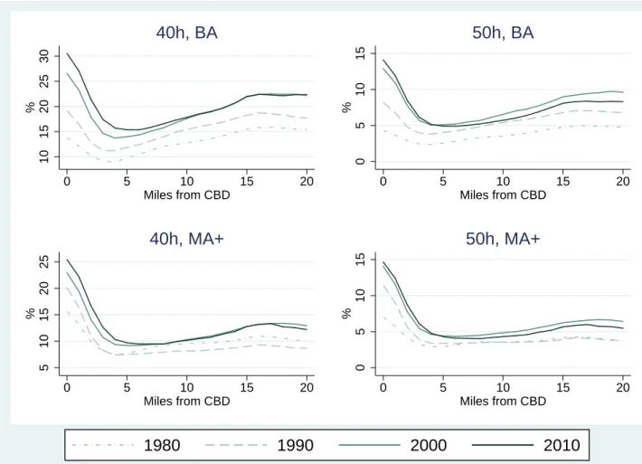
As for location, in 1980,F T(40, BA+) rose with distance to the city center, while
F T(40, M A+) declined slightly. In 2010, the population in the center was significantly
higher in the city center than the periphery, by 24 and 50 percent for F T(40, BA+)
F T(40, M A+) respectively. The growing proclivity to favor the city center is even
more pronounced among those working long (50+) hours, Table 1.14
Breaking down residence location by gender, we see that BA men working full time
were more likely to live away from the center than either skilled women or MA+ men,
Figures 4 and 5.
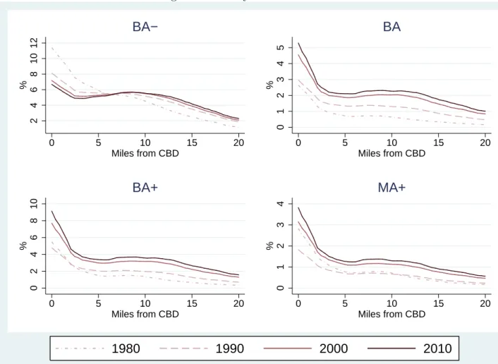
Location of jobs, distance to the CBD To investigate our premise that the
skilled work in the city center, we graph the distribution of jobs held by adults 25-55
(not conditional on hours) by the education level of the worker, Figure 6. We see that
all jobs are concentrated in the city core, but more so for the skilled than the unskilled.
Further, while there has been a “suburbanization” of jobs, it is particularly pronounced
for the unskilled: unskilled jobs decreased within 7 miles of the city center and grew
outside of that ring. Skilled jobs grew throughout.
Commuting time Average time spent commuting rose by 15 percent over the study
period [McKenzie and Rapino, 2011, figur 3]. Urban sprawl may be a factor. However,
as Figures 7-8 show, commuting time for workers at any given distance to the CBD
has increased, and the increase is in the range seen for the nation as a whole.
Turning to commuting patterns by distance to the CBD, we see that the BA+ group
spend more time commuting than the BA- group, suggestive of the importance of skill
match and concentration of skilled jobs in the CBD, Figure 9. Men spend more time
commuting than women, but the difference narrowed over the period. The greatest
13
Also true nationally for MA+ women working 40+ hours, see Appendix Table A1.
14
increase in commuting time is seen for BA women living at the outskirts. In 1980, they
seem to work locally, whereas by 2010 the catchment area appears to have widened,
consistent with a greater weight given to the skill match, Figure 8.
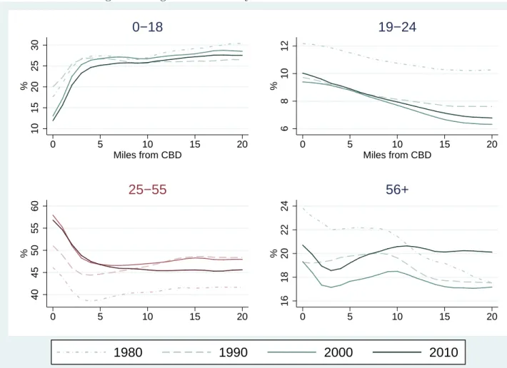
Age composition We now turn to the age distribution by distance. We find that
although urban revival has been tied to hipsters and empty nesters, the prime age
population dominates the city core, a tendency that increased over the study period,
Figure 10. In 1980, their share of the population was j-shaped, bottoming out around
4 miles from the CBD. In 2010, the j had fallen on its back – the share decreased
monotonically with distance, the sharpest decline being within the first five miles of
the CBD.
While young adults, 19 to 24 years old, have long favored the central city, their
presence decreased over the study period. Thus, this demographic does not seem to
be a prime driver of gentrification, perhaps not surprising considering their limited
purchasing power compared to the 25-55 age group.
As for ages 56 and above, this group has increased its presence in the population
overall but the growth in this demographic is concentrated 10 miles out of the CBD.
Within 10 miles of the CBD, there is a decrease. This was true of both the 56-65, and
the 66+ population, Table 1.
As regards children 0 to 18 years old, their share has declined nationally and in our
sample. The declined is particularly pronounced close to the city center, suggestive of
a limited role for the quality of public schools in shaping gentrification.
Turning to the fraction children in private school and we find that a higher fraction
of children attend private school in tracts close to the CBD and there was an increased
between 1990 and 2000, but declined between 2000 and 2010 (Figures A4-A5). Two
countervailing forces are likely at play. From a more affluent demographic close to the
CBD we would expect a higher fraction of children attending private schools. On the
other hand, the same demographic changes likely result in improved public schools.
The most striking change, however, is the erosion of the hump in private school
enrollment about 10 miles out of from the CBD evident in 1980. Since there are few
reflects a poorer suburban demographics.
Other demographics Table 1 also report tract means for income (total personal,
1980$), percent non-Hispanic white, black, and married. Over the period, income rose
by 25 percent, and as expected the gains were concentrated in tracts close to to the
CBD. In the 0-3 mile core, income rose by almost 80 percent.
The percent non-Hispanic white declined by 12 percentage points for our sample,
whereas the percent blacks increased only slightly (from 19.4 to 19.6 percent). In the
central city, however, the pattern was reversed: percent black declined while percent
non-Hispanic white held steady. As for marital status, marriage decline during the
study period, and in percentage terms the decline was steeper within 10 miles of the
city center (25 v. 15 percent).
4.1 Regression Analysis
Reduced form We start by investigating the reduced form effect of a demand shock
on housing prices by estimating the following regression:
P RICEijt=Zjt+f(distij)Zjt+f(distij) +αj+αt+ϵijt, (2)
whereP RICEijtis the housing price in tractiin cityjand yeart,Zjt is the exogenous
labor demand shock in cityjin yeart(cf. Equation 1) andf(distij) is a flexible function
ofdistij, the tract distance in miles to the CBD. The regression also includes year and
city fixed effects, αt and αj, or, alternatively, city-year fixed effects, αjt. We control
for distance specific characteristics throughf(distij) and allow for distance differential
impacts of Zjt through f(distij)×Zjt. Throughout, standard errors are clustered at
the city level, and tracts are weighted by their population size.
Table 2 presents the results. The first column shows the results from a bare-bones
version of Equation 2, where
f(distij) =d1ij+d2ij +d3ij (3)
the 3-10 mile radius ring, and the 10-20 mile ring respectively. (The 20-35 mile ring is
the reference area.)
We see that the effect of demand for skilled labor as measured by theZjtinstrument
is stronger close to the CBD, the estimated impact being 2.5 times larger in the core
than 3-10 miles out (588.9/234.5), and 6.7 times larger than in the 10-20 mile ring
(588.9/88.25).
Between 1980-2010, Z increased by about 13 percentage points,15
implying house
price changes of 75, 29 and 11 thousand 1980 USD in the 0-3 mile core, 3-10 mile,
and 10-20 mile rings respectively (relative to the 20-35 mile ring). The predicted price
changes line up closely with the observed price changes of 82, 30 and 4.5 thousand 1980
USD, respectively.
Results remain virtually unchanged when adding city-year fixed effects (column 2),
indicating common price responses to demand for skilled labor for the cities in our
sample over the study period.
Columns 3 and 4 us a quadratic or cubic specifications for f(distij). While more
parametric, these polynomials capture a similar effect of the demand shock: positive
but fading with distance.
Ideally, we would like to control for tract fixed effects but tracts change between the
censuses. We will construct a tract panel data set using cross-walk files but the fidelity
to the underlying tract characteristics is lower and therefore we favor results from the
repeated cross sectional sample.16
As a step towards tract fixed effects, we add vector
of city-specific distance fixed effectsg(distij) to Equation 2, that is, for columns 5-8 we
estimate
P RICEijt=Zjt+f(distij)Zjt+f(distij) +g(distij) +αj+αt+ϵijt, (4) 15
Table A2
16
where for each cityj we let:
g(distij) =
21
∑
k=1
βkjdkij (5)
where d1−d20 are indicator variables for the tract being [0,1), [1,2),...,[19-20) miles
away from the CBD (d21 indicates distance in the [20-35) mile range).
Results remain similar with this inclusion of “ring fixed effects,” columns 5-8.
First stage – T1st Table 3, shows the direct effect ofZjtonF T(h, e)ijt– the fraction
adults 25-55 in tracti, city j, year twho worked more that h= 40,50 hours per week
and had education e=BA+, M A+. We estimate a variant of Equation 2 where f(·)
is given by Equation 3 and the following three, successively more demanding, sets of
fixed effects: (1) city-year fixed effects; (2) city-distance fixed effects and year fixed
effects; and (3) city-distance fixed effects and city-year fixed effects.
Columns 1-3, upper panel, show the results for F T(40, BA+). We see a strong
positive effect of Z close to the CBD. The magnitude is reduced once city-specific
distance fixed effects are included (columns 2-3), but the qualitative flavor remains.
The point estimate from the third specification says that a 0.10 increase inZ leads to
a 3.3 percentage point higher increase in F T(40, BA+) in tracts 0-3 miles within the
CBD compared to tracts 20-35 miles out.
The results from the three other full-time measures are qualitatively similar results.
We now turn to other demographics that may change with the Bartik demand shifter
and plausibly influence housing prices. We estimate the same set of specifications as in
Table 3 but substitute the percent black, married, and personal income for the full-time
measure as the dependent variable.
Since these variables are correlated with the educational and employment status
of the population we expect to find a relationship. The reason we favor F T(·) over
these other variables is the direct causal link from growth in a skill intensive industry
to a more skilled and employed population. We view other demographic changes to be
incidental or derived from the primary relationship. Be that as it may, Table 4 presents
Starting with the percent black, we see that in the first specification (including
city-year fixed effects but not city-distance fixed effects), a higher Bartik reduces the
fraction blacks in tracts close to the city center. Adding city-distance fixed effects
(specifications two and three) halves the effect size but leaves the qualitative result
unchanged, Table 3, Columns 1-3.
Turning to non-Hispanic whites, we see a pronounced positive effect of the Bartik
demand shifter close to the CBD, Columns 4-6.
As for the percent married, in the first specification, we find no significant effect of
the Bartik demand shifter, Column 1, lower panel. Adding city-distance controls, we
find a small positive effect close to the CBD and a reduction in tracts 3-20 miles out,
Columns 2-3, lower panel.
Lastly, for personal income the estimated relationship is u-shaped with respect to
distance, with a trough in the 3-10 mile interval, Columns 4-6, lower panel.
OLS We can now engage our hypothesis that the emergence of centrality as a top
amenity is linked to high-income households being time starved. We focus on our
pre-ferred specification which controls for city-year and city-specific distance fixed effects:
P RICEijt=F T(h, e)ijt+f(distij)F T(h, e)ijt+g(distij) +αjt+ϵijt, (6)
where as beforef(distij) allows for the effect ofF T(h, e)ijtto vary with tract distance
to the CBD, and g(distij) is as in Equation 5.
We present three variations on Equation 6: (1) f(distij)F T(h, e)ijt is omitted;
(2) f(·) = distij; and (3) f(·) = distij +dist2ij. The OLS results from these three
specifications estimated for our four full-time measures are presented in Table 5. We
see that that the fraction full-time skilled workers in the tract and the tract’s housing
prices are positively related and the effect fades with distance to the CBD.
There are many reasons to question the interpretation of these OLS results, however.
Higher housing prices could prompt greater labor supply or the association could be
spurious. The central city could have been more attractive to the high-skill-low-leisure
population for reasons unrelated to commuting. Their presence could be driven by
which an urban aesthetics is embraced perhaps as a reaction against subdivisions and
cul-de-sacs.
IV We now turn to our IV estimates where we instrument our full-time skilled worker
measure by the Bartik demand shifter described in Section 3.2. Our identifying
assump-tion is that the Bartik demand shifter affects housing prices only through the posited
channel of raising the fraction of the population that is skilled and works full time.
The effect could stem directly from the purchasing power of a skilled, steadily
em-ployed population, or may be through the mores and preferences of this segment (e.g.,
regarding issues such as policing, liquor permits, bike lanes, etc.).
More worrying would be if demand growth for skilled labor affected other dimensions
that in turn moved housing prices. For instance, a higher Bartik may result in higher
tax revenues which in turn allow for better policing, infrastructure, or civic initiatives
that improve quality of life, and possibly more so close to the city center.
Pure racism presents another challenge. Consider the case of tipping points. It is
possible that a higher Bartik changes the demographics of a tract enough to make it tip.
For instance, prices in a centrally located tract may be low because its high proportion
blacks deters whites. As centrality gains salience, more whites move in, eventually
bringing the proportion blacks below the tipping point. Thence, white reservation
vanishes and prices take off. Note, however, that for the outlined mechanisms to be
a threat to our identification strategy, we need pure racism. Racial stereotypes that
merely reflect generalities regarding the behavior and preferences of a group based on
their education level, income, or employment status do not suffice.
With these caveats in mind, we now turn to our findings from estimating Equation
6 where F T(h, e)ijtand f(distij)F T(h, e)ijt are instrumented byZjt(1 +d1ij+d2ij+
d3ij). As in the case of the OLS regressions, we present three specifications: (1)
f(distij)F T(h, e)ijt is omitted; (2)f(·) =distij; and (3)f(·) =distij+dist2ij.
Throughout, the rudimentary specification in whichF T(·) is hypothesized to have
a uniform effect on housing prices regardless of distance to the CBD (and thus land
specifica-tions two and three.17
Both specifications estimate a positive effect of the fraction of
full-time skilled workers among the prime-age population (statistically significant at
the 0.1 percent level), and the effect is more pronounced closer to the CBD.
To gauge the economic significance of our proposed explanation for gentrification,
Figures 11 and 12 show the predicted housing price increases for the linear and square
specifications respectively. We see that both specification do a good job replicating the
actual price changes.
Robustness We now show the results from estimating the second specification in
a series of alternative samples as a robustness test (the first specification fails the
overidentification test, the third specification gives very similar results as the second
but the added interaction with distance squared is insignificant at conventional levels).
Motivated by the significant reduction in crime over the study period, we split
the cities according to the decline in crime (see Table A1). It is reassuring that our
results go through in both samples, although the strength of the first stage is somewhat
weakened. For the 40+ full-time measures, the effect size is noticeably smaller in the
low (crime reduction) sample, whereas for the 50+ full-time measures, the estimated
coefficients are similar in the two samples, Table 8, Columns 1 and 2 samples.
New York City is the largest US city, and may be exceptional in other ways too,
be it from the particularities forced geography, Manhattan Island in particular, the
concentration of the finance industry, the substantive presence of foreign buyers, or
the fact that it has a midtown and a downtown center. In order to gauge the extent
to which our results are driven by the presence of New York City, Column 3 presents
results from a sample where it has been excluded. Again, the results for the 50+ hours
full-time measures are very similar to those of the whole sample, while the estimated
effect size for our 40+ hours measure is reduced in magnitude (but remains statistically
very significant).
In the last three columns we present results from a tract panel data set constructed
using cross walk files from US2010.18
The thus constructed tracts, however, reflect the
17
The p-value of the Kleibergen-Paap LM test is below 1.7% throughout, rejecting the null that the model is underidentified.
18
underlying demographics with less fidelity (for further details, see the Appendix).
Column 4 presents results from including tract fixed effects and we find results to
be quite similar to the cross sectional sample (suggesting that the city-specific distance
fixed effects are passable substitutes for tract fixed effects).
Our main interest in a tract-level panel data set derives from the possibility that
initial conditions (other than distance) influence gentrification. In particular, we are
interested in the role of the initial racial composition of the tract.
To that end, we divide our panel data set according to whether the (constructed)
tract was above or below the median in terms of percent black in 1980 (the mean
and median values were 18.7 and 2.5 percent respectively, reflecting a high degree of
residential segregation).
We find results to be very similar in the two samples, Columns 5 and 6. That is,
once tract fixed effects and city-year fixed effects are controlled for, the effect of
full-time skilled workers on housing prices are estimated to be similar in tracts that had
few blacks (below 2.5 percent) and tracts that had a high fraction blacks (the implied
mean being close to 40 percent).
5
Discussion
For most of the 20th Century, suburbanization dominated the US urban landscape.
However, as the century drew to a close it was clear that a counter movement was
afoot. Today, gentrification has grown out of its erstwhile niche status to epitomize a
broad based rehabilitation of the central city as the place to work, live, and play.
The driving factor, we have proposed, can be found in a growing corps of
high-income-low-leisure households who by virtue of being time starved seek to locate close
to work. Thus, our paper adds urban renewal to the list of time-saving machinations
of modern life.
The ideas collated in this paper are by no means new. They hew closely to the
canonical models of urban development, and labor supply. The employment of a Bartik
demand shifter also follows a well-beaten path. To the best of our knowledge, however,
explanation for the reversal of suburbanization and to present comprehensive empirical
evidence to that effect.
We have focused on individual labor supply and lumped men and women together.
In the preliminary analysis we looked at men and women separately and found them to
yield similar results, possibly because the expansion of hours have been qualitatively
similar for skilled men and women. It is conceivable, however, that had the ever harder
working skilled men been paired with full time housewives, the situation would have
been wholly different.
The Suburbs Are Dead – Long Live the Suburbs Gentrification is about price
growth and changes to the housing stock, not population growth. Plenty of people will
find enduring value in the affordability and leafiness of the suburbs. However, other
aspects of suburban life may change.
For instance, between 2000 and 2010, Manhattan and Brooklyn poverty rates
de-clined by 10 percent, but rose on Staten Island (the most suburban of New York City’s
five boroughs).19
While more notable recently, poverty has been rising faster in suburbs
than cities since the 1980s [Kneebone and Berube, 2013].
To its critics, gentrification signifies the displacement of lower income households.
As the term suggests, displaced people show up somewhere else. The inner city, even
at its nadir, always had centrality going for it [Glaeser et al., 2000]. How do low-wage
workers, single-parents in particular, manage in suburban locations, areas built with
car ownership in mind and targeted to middle-class families with a stay-at-home wife?
Beyond the Burbs A topic of less social urgency but possibly affected by
gentrifica-tion is the secondary home market. Gentrificagentrifica-tion may breath new life into towns two
or three hours away from the city. Too remote to be commuter towns, such places can
be desirable weekend destinations. As more high-income families live in apartments
rather than free standing houses, demand for second homes may pick up.
The only way is up? Urban sprawl had cheap housing going for it. Is the future
one of ever rising land rents?
19
East Asia may offer guidance. Japan and South Korea are both developed
industri-alized countries, but gentrification appears to have been largely absent [Waley, 1997].
Several factor may account for this, including close to zero population growth and low
labor force participation of married women. More replicable, however, is the vertical
urban landscape built around mass transportation, notably trains. High density and
rail connectedness ease the pressure on land rents both by packing in and
transport-ing more people within any given area and by allowtransport-ing for multiple centers within the
urban core. While the sky may not be the limit, US cities still have a lot of head room.
References
Daniel Aaronson. Neighborhood dynamics. Journal of Urban Economics, 49(1):1 – 31, 2001.
Mark Aguiar and Erik Hurst. Measuring trends in leisure: The allocation of time over five decades. Quarterly Journal of Economics, 122(3):969–1006, August 2007.
Mark Aguiar and Erik Hurst. The Increase in Leisure Inequality 19652005. The AEI Press, 2009.
David H. Autor, Lawrence F. Katz, and Melissa S. Kearney. Trends in U.S. wage inequality: Revising the revisionists. The Review of Economics and Statistics, 90(2): 300–323, May 2008.
C. F. Baum. Enhanced routines for instrumental variables/generalized method of moments estimation and testing. Stata Journal, 7(4):465–506(42), 2007. URL http://www.stata-journal.com/article.html?article=st0030_3.
Paul Beaudry, Mark Doms, and Ethan Lewis. Should the Personal Computer Be Considered a Technological Revolution? Evidence from US Metropolitan Areas.
Journal of Political Economy, 118(5):988–1036, October 2010.
Christopher R. Berry and Edward L. Glaeser. The divergence of human capital levels across cities. Papers in Regional Science, 84(3):407 – 444, 2005. ISSN 10568190.
Dan Black, Gary Gates, Seth Sanders, and Lowell Taylor. Why do gay men live in San Francisco? Journal of Urban Economics, 51(1):54 – 76, 2002.
Willem R. Boterman, Lia Karsten, and Sako Musterd. Gentrifiers settling down? pat-terns and trends of residential location of middle-class families in Amsterdam. Hous-ing Studies, 25(5):693 – 714, 2010.
Juliet Carpenter and Loretta Lees. Gentrification in new york, london and paris: An international comparison. International Journal of Urban and Regional Research, 19 (2):286, 1995.
Janice Compton and Robert A. Pollak. Why are power couples increasingly concen-trated in large metropolitan areas? Journal of Labor Economics, 25(3):pp. 475–512, 2007.
Dora Costa and Matthew E. Kahn. Power couples: Changes in the locational choice of the college educated, 1940-1990.Quarterly Journal of Economics, 115(4):1287–1315, November 2000.
David M. Cutler, Edward L. Glaeser, and Jacob L. Vigdor. The rise and decline of the American ghetto. Journal of Political Economy, 107(3):455–506, JUN 1999.
Morris A. Davis and Jonathan Heathcote. The price and quantity of residential land in the united states. Journal of Monetary Economics, 54(8):2595 – 2620, 2007.
Rebecca Diamond. The determinants and welfare implications of US workers’ diverging location choices by skill: 1980-2000. American Economic Review, Forthcoming.
Riccardo DiCecio, Kristie M. Engemann, Michael T. Owyang, and Christopher H. Wheeler. Changing trends in the labor force: A survey. Federal Reserve Bank of St. Louis Review, 90(1), January/February 2008.
John J. III Donohue and Steven D. Levitt. The impact of legalized abortion on crime.
Quarterly Journal of Economics, 116(2):379–420, May 2001.
Lena Edlund and Rohini Pande. Why have women become left-wing: The political gender gap and the decline in marriage. Quarterly Journal of Economics, 117:917– 961, August 2002.
Alan Ehrenhalt. The Great Inversion and the Future of the American City. Vintage, paperback edition, 2013.
Giovanni Favara and Jean Imbs. Credit supply and the price of housing. American Economic Review, 105(3):958–92, 2015.
Raquel Fernndez and Joyce Wong. Unilateral divorce, the decreasing gender gap, and married women’s labor force participation. American Economic Review, 104(5):342– 47, 2014.
Christopher Foote and Christopher Goetz. The impact of legalized abortion on crime: Comment. Quarterly Journal of Economics, 123(1), February 2008.
Edward L. Glaeser, Matthew E. Kahn, and Jordan Rappaport. Why do the poor live in cities? Working Paper 7636, National Bureau of Economic Research, April 2000.
Edward L. Glaeser, Jed Kolko, and Albert Saiz. Consumer city. Journal of Economic Geography, (1):27–50, 2001.
Edward L. Glaeser, Joshua D. Gottlieb, and Kristina Tobio. Housing booms and city centers. Working Paper 17914, National Bureau of Economic Research, March 2012.
Edward L. Glaeser, Joseph Gyourko, and Albert Saiz. Housing supply and housing bubbles. Journal of Urban Economics, 64(2):198–217, SEP 2008. ISSN 0094-1190. doi: {10.1016/j.jue.2008.07.007}.
Jeremy Greenwood and Boyan Jovanovic. The information-technology revolution and the stock market. The American Economic Review, 89(2):pp. 116–122, 1999.
Jeremy Greenwood, Nezih Guner, Georgi Kocharkov, and Cezar Santos. Marry your like: Assortative mating and income inequality. American Economic Review, 104(5): 348 – 353, 2014.
Veronica Guerrieri, Daniel Hartley, and Erik Hurst. Within-city variation in urban decline: The case of Detroit. American Economic Review: Papers and Proceedings, 102(3):120126, 2012.
Veronica Guerrieri, Daniel Hartley, and Erik Hurst. Endogenous gentrifcation and housing price dynamics. Journal of Public Economics, 100:45–60, 2013.
Joseph Gyourko, Christopher Mayer, and Todd Sinai. Superstar cities. American Economic Journal: Economic Policy, 5(4):167–99, 2013.
Bradley T. Heim. The incredible shrinking elasticities: Married female labor supply, 1978-2002. The Journal of Human Resources, 42(4):pp. 881–918, 2007.
Bart Hobijn and Boyan Jovanovic. The information-technology revolution and the stock market: Evidence. The American Economic Review, 91(5):pp. 1203–1220, 2001.
Kenneth T. Jackson. Crabgrass Frontier. Oxford University Press, 1985.
Jane Jacobs. The Death and Life of Great American Cities. Random House, New York, 1961.
William R. Johnson. House prices and female labor force participation. University of Virginia, January 2012.
Chinhui Juhn and Kevin M. Murphy. Wage inequality and family labor supply.Journal of Labor Economics, 15(1):72–97, January 1997.
Matthew E. Kahn. Gentrification trends in new transit-oriented communities: Evidence from 14 cities that expanded and built rail transit systems. Real Estate Economics, 35(2):155–182, Sum 2007.
Lawrence F. Katz and Kevin M. Murphy. Changes in the relative wages, 1963-87: supply and demand factors.Quarterly Journal of Economics, 107(1):35–78, February 1992.
Elizabeth Kneebone and Alan Berube. Confronting Suburban Poverty in America. James A. Johnson Metro. Brookings Institution Press, 2013.
Wojciech Kopczuk, Emmanuel Saez, and Jae Song. Uncovering the American dream: Inequality and mobility in social security earnings data since 1937. NBER Working Paper, (13345), 2008.
Peter J. Kuhn and Fernando A. Lozano. The expanding workweek? understanding trends in long work hours among U.S. men, 1979-2004. Discussion Paper 1924, IZA, 2006.
Janice F. Madden and Michelle J. White. Spatial implications of increases in the female labor force: A theoretical and empirical synthesis. Land Economics, 56(4):432–446, Nov. 1980.
Janice Fanning Madden. Consequences of the growth of the two-earner eamily urban land use and the growth in two-earner households. American Economic Review, 70 (2):191–197, 1980.
Scott C. McDonald. Does gentrification affect crime rates. Crime & Just., 8:163, 1986.
Ellen McGrattan and Richard Rogerson. Changes in the distribution of family hours worked since 1950. Research Department Staff Report 397, Federal Reserve Bank of Minneapolis, 2008.
Brian McKenzie and Melanie Rapino. Commuting in the united states, 2009. American Community Survey Reports ACS-15, Census Bureau, Washington, DC, 2011.
Peter Mieszkowski and Edwin S. Mills. The causes of metropolitan suburbanization.
Journal of Economic Perspectives, 7(3):135–147, Sum 1993.
Enrico Moretti. Real wage inequality.American Economic Journal-Applied Economics, 5(1):65–103, Jan 2013.
National Association of Realtors. Home buyer and seller generational trends. Technical report, 2014. http://www.realtor.org/sites/default/files/reports/2014/2014-home-buyer-and-seller-generational-trends-report-full.pdf.
Jordan Rappaport. Monocentric city redux. Research Working
Paper 14-09, The Federal Reserve Bank of Kansas City, 2014.
https://www.kansascityfed.org/publicat/reswkpap/pdf/rwp14-09.pdf.
Jessica Wolpaw Reyes. Environmental policy as social policy? The impact of childhood lead exposure on crime. B E Journal of Economic Analysis & Policy, 7(1), 2007.
Gilles Saint-Paul. Bobos in paradise: Urban politics and the new economy. Discussion Paper 10879, Centre for Economic Policy Research, 2015.
Thomas C. Schelling. Models of segregation. American Economic Review, 59(2):488– 493, 1969. ISSN 0002-8282.
Christine R. Schwartz. Earnings inequality and the changing association between spouses earnings. American Journal of Sociology, 115(5):pp. 1524–1557, 2010.
James H. Stock and Motohiro Yogo. Testing for weak instruments in linear iv regres-sion. In Donald W. K. Andrews and James H. Stock, editors, Identification and Inference for Econometric Models: Essays in Honor of Thomas Rothenberg. Cam-bridge University Press, 2005. http://dx.doi.org/10.1017/CBO9780511614491.006.
Stijn Van Nieuwerburgh and Pierre-Olivier Weill. Why has house price dispersion gone up? The Review of Economic Studies, 77(4):1567–1606, 2010.
Paul Waley. Tokyo - patterns of familiarity and partitions of difference. American Behavioral Scientist, 41(3):396–429, 1997.
Graphs
Figure 1: Home Prices by location
50
100
150
200
250
1980USD (000)
0
5
10
15
20
Miles from CBD
1980
1990
2000
2010
Figure 2: % Working full time, 40h/week, by sex and education
20
30
40
50
60
70
80
90
%
1940 1950 1960 1970 1980 1990 2000 2010
Men & BA− Men & BA+
Women & BA− Women & BA+
Note: Ages 25-55.
Figure 3: % Working full time, 50h/week, by sex and education
0
10
20
30
40
50
%
1940 1950 1960 1970 1980 1990 2000 2010
Men & BA− Men & BA+
Women & BA− Women & BA+
Note: Ages 25-55.
Figure 4: % full time and skilled among men 25-55
10
15
20
25
30
%
0 5 10 15 20
Miles from CBD
40h, BA
0
5
10
15
%
0 5 10 15 20
Miles from CBD
50h, BA
5
10
15
20
25
%
0 5 10 15 20
Miles from CBD
40h, MA+
0
5
10
15
%
0 5 10 15 20
Miles from CBD
50h, MA+
1980
1990
2000
2010
Figure 5: % full time and skilled among women 25-55
5
10
15
20
25
%
0 5 10 15 20
Miles from CBD
40h, BA
0
2
4
6
8
10
%
0 5 10 15 20
Miles from CBD
50h, BA
0
5
10
15
20
25
%
0 5 10 15 20
Miles from CBD
40h, MA+
0
2
4
6
8
10
%
0 5 10 15 20
Miles from CBD
50h, MA+
1980
1990
2000
2010
Figure 6: Jobs by skill
2
4
6
8
10
12
%
0 5 10 15 20
Miles from CBD
BA−
0
1
2
3
4
5
%
0 5 10 15 20
Miles from CBD
BA
0
2
4
6
8
10
%
0 5 10 15 20
Miles from CBD
BA+
0
1
2
3
4
%
0 5 10 15 20
Miles from CBD
MA+
1980
1990
2000
2010
Universe: filled jobs within 35 miles of the CBD.
Figure 7: Commuting time by education and residence location, men
20
25
30
35
Minutes
0 5 10 15 20
Miles from CBD
BA−
20
25
30
35
Minutes
0 5 10 15 20
Miles from CBD
BA
20
25
30
35
Minutes
0 5 10 15 20
Miles from CBD
BA+
20
25
30
35
Minutes
0 5 10 15 20
Miles from CBD
MA+
1980
1990
2000
2010
One way, door-to-door.
Universe: Men 25-55 who work away from home.
Figure 8: Commuting time by education and residence location, women
22
24
26
28
30
Minutes
0 5 10 15 20
Miles from CBD
BA−
22
24
26
28
30
Minutes
0 5 10 15 20
Miles from CBD
BA
22
24
26
28
30
Minutes
0 5 10 15 20
Miles from CBD
BA+
22
24
26
28
30
Minutes
0 5 10 15 20
Miles from CBD
MA+
1980
1990
2000
2010
One way, door-to-door.
Universe: Women 25-55 who work away from home.
Figure 9: Commuting time, by sex, education, and residence location
20
25
30
35
Minutes
0 5 10 15 20
Miles from CBD
1980
20
25
30
35
Minutes
0 5 10 15 20
Miles from CBD
1990
20
25
30
35
Minutes
0 5 10 15 20
Miles from CBD
2000
20
25
30
35
Minutes
0 5 10 15 20
Miles from CBD
2010
BA−
BA
MA+
BA−
BA
MA+
Men Women
Figure 10: Age distribution by residence location
10
15
20
25
30
%
0 5 10 15 20
Miles from CBD
0−18
6
8
10
12
%
0 5 10 15 20
Miles from CBD
19−24
40
45
50
55
60
%
0 5 10 15 20
25−55
16
18
20
22
24
%
0 5 10 15 20
56+
1980
1990
2000
2010
Universe: Residents residing x= 0,1, ...18,19,20−35 miles from the CBD.
Figure 11: Predicted v. Actual Price increase, ‘000 1980$
0
50
100
150
1980USD (000)
0 5 10 15 20
Miles from CBD
Figure 12: Predicted v. Actual Price increase, ‘000 1980$
−50
0
50
100
150
1980USD (000)
0 5 10 15 20
Miles from CBD
Tables
Table 1: Summary Statistics
(1) (2) (3) (4) (5)
Distance to the CBD (miles)
Variable Year d1=[0,3] d2=(3,10] d3=(10,20] d4=(20,35) [0,35)
House price 1980 66.64 79.16 108.23 114.06 92.5
(’000 1980$) 2010 154.77 115.07 119.22 120.5 120.54
∆ 88.13 35.91 10.99 6.44 28.04
FT(40,BA+) 1980 13.78 12.92 15.19 15.05 14.05
2010 35.13 23.15 27.22 28.29 26.62
∆ 21.35 10.23 12.03 13.24 12.57
FT(40,MA+) 1980 6.37 5.42 6.12 5.64 5.77
2010 15.5 8.92 10.1 10.35 10.13
∆ 9.13 3.5 3.98 4.71 4.36
FT(50,BA+) 1980 4.03 3.43 4.3 4.44 3.92
2010 14.32 7.25 8.81 9.69 8.86
∆ 10.29 3.82 4.51 5.25 4.94
FT(50,MA+) 1980 2.29 1.82 2.06 1.93 1.96
2010 7.28 3.4 3.8 4.02 3.95
∆ 4.99 1.58 1.74 2.09 1.99
Income 1980 10.53 12.06 14.25 14.3 12.94
(’000 1980$) 2010 17.98 13.99 17.22 18.77 16.53
∆ 7.45 1.93 2.97 4.47 3.59
White 1980 48.99 62.43 75.61 85.73 68.87
2010 44.97 38.81 53.91 66.37 51.06
∆ -4.02 -23.62 -21.7 -19.36 -17.81
Black 1980 32.89 23.61 13.41 6.78 18.7
2010 25 27.22 15.43 7.49 18.25
∆ -7.89 3.61 2.02 0.71 -0.45
Married 1980 46.29 62.67 72.22 77.35 66.32
2010 36.13 48.25 60.72 66.59 56.14
Table 1: Summary Statistics, continued
(1) (2) (3) (4) (5)
Distance to the CBD (miles)
Variable Year d1=[0,3] d2=(3,10] d3=(10,20] d4=(20,35) [0,35) Ages:
0-5 1980 8.03 7.85 7.51 8.23 7.82
2010 6.99 8.32 8.04 8.12 8.08
∆ -1.04 0.47 0.53 -0.11 0.26
6-12 1980 9.04 9.56 10.09 11.02 9.9
2010 6.58 9.02 9.63 10.12 9.33
∆ -2.46 -0.54 -0.46 -0.9 -0.57
13-18 1980 8.97 9.66 10.62 11.35 10.16
2010 6.05 8.12 8.64 8.83 8.33
∆ -2.92 -1.54 -1.98 -2.52 -1.83
19-24 1980 12.45 11.21 10.41 10.46 10.97
2010 10.31 8.58 7.36 6.77 7.84
∆ -2.14 -2.63 -3.05 -3.69 -3.13
25-55 1980 39 38.7 40.52 40.81 39.63
2010 50.45 45.53 44.64 44.63 45.34
∆ 11.45 6.83 4.12 3.82 5.71
56-65 1980 9.74 10.86 10.67 9.21 10.42
2010 9.67 9.88 10.7 10.88 10.39
∆ -0.07 -0.98 0.03 1.67 -0.03
66- 1980 12.76 12.16 10.18 8.93 11.09
2010 9.95 10.55 10.99 10.64 10.68
∆ -2.81 -1.61 0.81 1.71 -0.41
Private school:
6-12 1980 21.71 25.55 19.89 12.99 21.41
2010 20.38 15.75 14.25 12.04 14.65
∆ -1.33 -9.8 -5.64 -0.95 -6.76
13-18 1980 18.3 19.59 14.36 9.48 16.23
2010 19.22 15.35 12.89 10.45 13.57
∆ 0.92 -4.24 -1.47 0.97 -2.66
Commute 1980 23.54 26.59 27.76 26.31 26.6
(one-way) 2010 25.68 29.15 29.2 30.46 29.24
∆ 2.14 2.56 1.44 4.15 2.64