APPLYING THE ARTIFICIAL NEURAL NETWORK METHODOLOGY FOR FORECASTING THE TOURISM TIME SERIES

APPLYING THE ARTIFICIAL NEURAL NETWORK METHODOLOGY

FOR FORECASTING THE TOURISM TIME SERIES

Paula Fernandes1, João Teixeira2

1

Department of Economics and Management, School of Technology and Management Polytechnic Institute of Bragança, Campus de Sta. Apolónia,

Apartado 134, 5301-857 Bragança, Portugal, e-mail: pof@ipb.pt 2

Department of Electrical Engineering, School of Technology and Management Polytechnic Institute of Bragança, Campus de Sta. Apolónia,

Apartado 134, 5301-857 Bragança, Portugal, e-mail:joaopt@ipb.pt

Abstract. This paper aims to develop models and apply them to sensitivity studies in order to predict the demand. It provides a deeper understanding of the tourism sector in Northern Portugal and contributes to already existing econometric studies by using the Artificial Neural Networks methodology. This work’s focus is on the treatment, analysis, and modelling of time series representing “Monthly Guest Nights in Hotels” in Northern Portugal re-corded between January 1987 and December 2005. The model used 4 neurons in the hidden layer with the logis-tic activation function and was trained using the Resilient Backpropagation algorithm. Each time series forecast depended on 12 preceding values. The analysis of the output forecast data of the selected ANN model showed a reasonably close result compared to the target data.

Keywords: artificial neural networks, time series forecasts, tourism, backpropagation, feedforward, training.

1. Introduction

Several empirical studies in the tourism scientific area have been performed and published in the last decades. These studies agree that the forecast process in the tourism sector must be done with particular care.

In this context, and related to tourism demand in Northern Portugal, a study has been carried out with the reference temporal sequence –“Monthly Guest Nights in Hotels”.

The object sequence – “Monthly Guest Nights in Hotels” consist in the registered number of the over-night in the all category Hotels of the North region of Portugal (basically in the region of North of Douro River) in each month.

The study consisted in develop a model for pre-dict the next year sequence knowing the values of the previous year. For this purpose the model used is supported in Artificial Neural Networks (ANN) meth-odology and was developed in the Matlab environment. The ANN methodology was inspired in the bio-logic theories of human brain function [1]. The human brain is composed of several non-linear processors densely interconnected operating in parallel.

This paper is organized in the following struc-ture: first, there is an overview section that examines the theoretical foundation of neural networks. Then, the

following section, in particular, assesses the use of ANN models as a forecasting tool for business applica-tions. Based on the theoretical analysis, a neural net-work is developed for forecasting tourism demand in Northern Portugal. Real data from official publications in Portugal is used for the neural network development. The model development process, the empirical and analysis results of forecasting are described in sec-tion 4. The quality of forecasting results is measured in mean absolute percentage error. Some concluding remarks are given in the final section.

2. Analogy between artificial neuron and biological neuron

a. Information processing occurs at several simple elements that are called neurons;

carries them away through the synapse to the dendrites of neighbouring neurons.

b. Signals are passed between neurons over con-nection links;

Because a neuron has a large number of den-drites/synapses, it can receive and transmit many sig-nals at the same time; these sigsig-nals may either excite or inhibit the firing of the neuron [2]. This basic system of signal transfer was the fundamental step of early neuro-computing development and the operation of the build-ing unit of Artificial Neural Networks.

c. Each connection link has an associated weight, which, in a typical neural net, multiplies the signal transmitted;

d. Each neuron applies an activation function (usu-ally nonlinear) to its net input (sum of weighted input signals) to determine its output signal. Through replicate learning process and associa-tive memory, the ANN model can accurately classify information as pre-specified pattern. A typical ANN consists of a number of simple processing elements called neurons, nodes or units. Each neuron is con-nected to other neurons by means of directed commu-nication links. Each connection has an associated weight. The weights are the parameters of the model being used by the net to solve a problem. ANNs are usually modelled into one input layer, one or several hidden layers, and one output layer [10]. Fig 2 demon-strates a simplified neural network with three layers.

In Fig 2, each node in the hidden layer computes

Fig 1. Schematic of biological neuron [2]

( 1, 2, 3 j

y j= ) according to expression (1) [9]: The basic analogy between artificial neuron and

biological neuron is that the connections between nodes correspond to the axons and dendrites, the connection weights represent the synapses and the threshold ap-proximates the activity in the soma.

2

1

j i ji

i

f x w

=

=

_∑

(1)

(yj)

In addition, a sigmoid function , in the fol-lowing form, is used to transform the output that is limited into an acceptable range. The purpose of a

sigmoid function is to prevent the output being too

large, as the value of

3. Neural Networks Approach

The theory of neural network computation pro-vides interesting techniques that mimic the human brain and nervous system, like we showed before. Neural networks are an information technology capable of representing knowledge based on massive parallel processing and pattern recognition based on past ex-perience or examples. The artificial neural networks have been extensively studied and used in time series forecasting. The pattern recognition ability of a neural network makes it a good alternative classification and forecasting tool in business applications [3, 4, 5]. In addition, a neural network is expected to be superior to traditional statistical methods in forecasting because a neural network is better able to recognize the high-level features, such as serial correlation, if any, of a training set.

j

y _{(for j=1, 2, 3) must fall}

be-tween 0 and 1:

1

1 j

j f

y

e−

=

+ (2)

Finally, in the node of the output layer in Fig 2 is obtained by the following function:

Y

(3) 3

1

j j j

Y

y w

=

=

∑

An additional advantage of applying a neural network to forecasting is that a neural network can capture the non-linearity of samples in the training set [2, 6, 7]. Using a neural network to forecast non-lnear tourist behaviour could achieve a lower mean absolute percentage error, lower cumulative relative absolute error, and lower root mean square error than classical models [6, 8].

Artificial Neuronal Networks has been developed as generalizations of mathematical models of human cognition or neural biology, based on the assumptions that [9]:

W13

W22

W23

W21

W12

W2 W3

W1

W11

Output Layer

Hidden Layer

Input Layer

y1 y2 y3

Y

X1 X2

Nodes in the input layer represent independent parameters of the system. The hidden layer is used to add an internal representation handling non-linear data.The output of the neural network is the solution for the problem. A feedforward neural network learns from a supervised training data to discover patterns connecting input and output variables. Feedforward recall is a one-directional information processing neural network in which the signal flows from the input units to the output units in a forward direction [11, 12, 13].

Much of the current interest in the neural network technique forecasting tool can be traced to the devel-opment of the backpropagation learning algorithm. This algorithm gives the network the ability to form and modify its own interconnections in a way that often rapidly approaches a goddness-of-fit optimum. The technique was first developed by Werbos and further advance by Rumelhart, Hinton and Williams [9].

Many variants of Backpropagation training algo-rithm were developed . In our case we adopted the

Resilient Backpropagation, because it can combine fast

convergence, stability and generally good results [14]. Usually, the learning process involves the follow-ing stages [4, 6]:

1. Assign random numbers to the weights; 2. For every element in the training set, calculate

output using the summation functions embed-ded in the nodes;

3. Compare computed output with observed val-ues;

4. Adjust the weights and repeat steps (2) and (3) if the result from step (3) isn’t less than a threshold value; alternatively, this cycle can be stopped early by reaching a predefined number of iterations, or the performance in a validation set does not improve.

5. Repeat the above steps for other elements in the training set.

4. Tourism demand forecasting in Northern Portugal

4.1. Methods and procedures

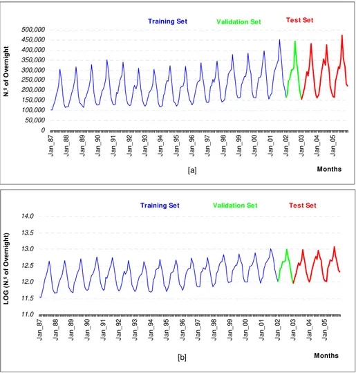
For the selection of data we used the secondary source published in the Portuguese National Statistical Institute. According the study published by Fernandes [6] and Fernandes and Teixeira [5], the original time series suggests a power transformation (Fig 3a). There-fore we take logarithms of the data to stabilize the seasonality and variance, and we have another time series that was used during the work, namely Trans-formed Original Data (TOD) (Fig 3b).

The ANN model used in this study is the standard three-layer feedforward network. Since the one-step- ahead forecasting is considered, only one output node is employed. The activation function for hidden nodes

is the logistic function [Logsig]:

( )

1 ( )

1 e x

f x = ₋

+ ; and

for the output node the identity function (pure linear function) [Lin]: f x( )=x.

Bias terms are used in both hidden and output layer’s nodes. The fast Resilient Backpropagation algorithm provide by the MATLAB neural network toolbox is employed in training process. The ANN is randomly initialised with weights and bias values. For selecting the architecture several experiments with different architectures were carried out (train and test) and the better architectures were selected according to the results in a validation set using hundreds of training sessions. So, the architecture consists of 12 input nodes in the entrance layer, 4 hidden nodes in the second layer and one node in the output layer – (1–12;4;1). The input of the model consists of the 12 previous numbers – corresponding to the last 12 months over-nights. The output is the predicted overnights for the next month. The selection of this model is supported in the author’s work Fernandes [6] and Fernandes and Teixeira [5].

To make monthly predictions we have combined the following assumptions: consider as delayed inputs the most previous observations of the month we are predicting; due to the seasonal behaviour of the series we use a period of twelve months.

The data set was divided in a sub-set for training, a sub-set for validation and a sub-set for test. The data set between January 1988 until December 2001 (in a total of 168 observations) was used for training. In the training process of an ANN different end points are achieved, although with similar performance, for dif-ferent initial values. Therefore, several training ses-sions for each identified situation have been performed with different initial weights. From this number of training sessions we retain the ANN (concerning its weights) that obtain better forecast results in each situation under the validation set (see [6]).

It must be noted that the data between January and December 1987 was used as the input data for predicting January 1988 till December. The data be-tween January and December 2002 was used for the validation set. This set is used for early stop training if the root mean squared error (RMSE) does not decrease in a number of 5 training iterations. This early stop training condition avoids the ANN to over fit the train-ing data without improvements in a data not used in the training phase. Finally, the data between January 2003 till December 2005 (36 observations) was used as the target. This data was never seen under the train-ing and selection process and was only used to present the results of the model with never seen data.

For an ANN model the prediction equation for

computing a forecast of using selected past observa-tions can be written as [6]:

t Y

(5)

2,1 1,

1 1

n m

t j ij t i

j i

Y b w f W y₋ b

= =

⎛ ⎞

= + _⎜ + _⎟

⎝ ⎠

∑

∑

j

where,m is the number of input nodes; is the num-ber of hidden nodes;

n

such as the logistic, used in the hidden layer nodes;

{

w_j,j=0,1,…,n

}

is a vector of weights from the

hidden to output nodes;

the agreement index, according to equation (5). The other agreement index used in this paper is the coeffi-cient of correlation between the observed and predi-cated values, equation (6).

{

W i_ij, =0,1,K, ;m j=1, 2,K,n

}

are weights from the

input to hidden nodes; and

(

)

2 1 _; n t t t A P RMSE n = − =

∑

w h er e A is t h e t ar g et v alu e ,

P d en o t es t h e v alu e of p r ed ict ion an d n t h e t o t al n u m b er o f o b ser v at io n s.

2,1

b

b

_1,j are the bias asso-ciated with the nodes in output and hidden layers, respectively.

The equation shows a linear transfer function used in the output node and the resilient backpropaga-tion algorithm was used for training the ANN.

4.2. Empirical results

In this section we will observe the results of each ANN under the test set. For this purpose we will com-pare the predicted data of each ANN with the target values for the last three years 2003 to 2005 (the tests set). We should emphasize that the target data is the original data of the time series and was never seen by the model in the training phase. The selection process of the better ANN is governed by the minimum RMSE in the training set (see [6]).

In order to compare the performance, the RMSE between the observed and predicted values are used as

(5)

(

)(

)

(

) (

)

1 , 2 2 1 . ; n t t t A P _n

t t

t

A A P P

r

A A P P

= = − − = − −

∑

∑

where A is t he t arget value ,

P denot es t he value of predict ion and n t he t ot al num ber of observat ions

(6)

Comparing the results, presented in Table 1, of the prediction and considering that this model resulted from a selection of several different architectures we can say that the final results are stable and has an interesting performance, but we can never say that this is the better model. Therefore, this model is selected based only in the training set.

N .º of O v e rni ght 0 50,000 100,000 150,000 200,000 250,000 300,000 350,000 400,000 450,000 500,000 J a n_ 87 J a n_ 88 J a n_ 89 J a n_ 90 J a n_ 91 J a n_ 92 J a n_ 93 J a n_ 94 J a n_ 95 J a n_ 96 J a n_ 97 J a n_ 98 J a n_ 99 J a n_ 00 J a n_ 01 J a n_ 02 J a n_ 03 J a n_ 04 J a n_ 05 Months Validation Set

Training Set Test Set

[a] LO G (N .º of O v e rni ght) 11.0 11.5 12.0 12.5 13.0 13.5 14.0 J an _87 J an _88 J an _89 J an _90 J an _91 J an _92 J an _93 J an _94 J an _95 J an _96 J an _97 J an _98 J an _99 J an _00 J an _01 J an _02 J an _03 J an _04 J an _05 Months

Training Set Validation Set Test Set

[b]

Table 1. Results of ANN model.

Performance Measured Time Training set

(n=168)

Test set

Serie (n=36)

r RMSE r RMSE

TOD 0.989 12.268 0.9615 21.8715

We should look now at the performance in the test set. Regarding the performance in the test set presented in Table 1 the RMSE becomes deteriorated now, but the correlation coefficient stills at a relatively high level.

The summary statistics for the out-of-sample (data used as the test set) forecasting performance of model are given in Table 2. MAPE is the Mean Abso-lute Percentage Error given by the expression (7).

. 1

ˆ 1

100 N

t t

t t

Y Y MAPE

Y N

− ∑ =

= × (6)

Table 2. Out-of-sample (test set) forecasting error measures.

Year r RMSE MAPE (%)

2003 0.983 18.969 6.39 %

2004 0.958 23.065 5.77 %

2005 0.967 23.315 6.89 %

Judged by all three overall accuracy measures and across three test sets we observe that the forecast-ing performance of this model in 2005 is not as good as in the other years but still at the very same level of accuracy. Therefore, according to the Criteria of MAPE for Model Evaluation in Lewis [15], the predicted data with the selected model has a highly accurate forecast, because the results are lower than 10 %.

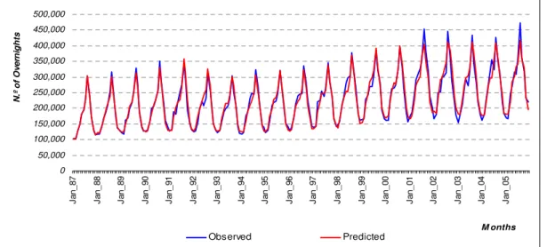
Fig 4 displays the original and predicted time se-ries for the entire sequence. As expected the model predicts better the values under the period of training set than for the period of the test set, that were not seen previously. We can observe an additional difficulty for the model imposed by the fact that years 2001 till 2005

have had an increasing number of overnights, and this increasing phenomenon was present in the training set only in 2001 and was difficulty to reflect for the fol-lowing years. This phenomenon was due to the fact that the city of Guimarães and the Douro Region were considered World Cultural Heritage, and the city of Porto was the European Capital of Culture in 2001.

5. Conclusions

This paper presents the process of modelling tourism demand for the north of Portugal, using an artificial neural network model. The time series was considered in the logarithmic transformed data. This series was separated into a training data set to train the neural network, in a validation set, to stop the training process earlier and a test data set to examine the level of forecasting accuracy.

The model has 4 neurons in the hidden layer with the logistic activation function and was trained using

the Resilient Backpropagation algorithm(a variation of

backpropagation algorithm). The ANN model has the 12 preceding values as the input. The analysis of the output forecast data of the selected ANN model showed a reasonably close result compared to the target data. In other words, the model produced, according to the criteria of MAPE a highly accurate forecast. Therefore it can be considered adequate for the purpose of predic-tion in the reference time series. But the best model in most real world forecasting situations should be the one that is robust and accurate for a long time horizon and thus users can have confidence to use the model fre-quently.

To test the robustness of a model, it is critical to employ multiple years in the test set.

Finally and considering the results, the artificial neural network based models represent an effective alternative to classical models in tourism forecasting. This methodology becomes interesting to forecast because it allows the use of a non linear model for seasonal time series.

0 50,000 100,000 150,000 200,000 250,000 300,000 350,000 400,000 450,000 500,000

Ja

n

_

8

7

Ja

n

_

8

8

Ja

n

_

8

9

Ja

n

_

9

0

Ja

n

_

9

1

Ja

n

_

9

2

Ja

n

_

9

3

Ja

n

_

9

4

Ja

n

_

9

5

Ja

n

_

9

6

Ja

n

_

9

7

Ja

n

_

9

8

Ja

n

_

9

9

Ja

n

_

0

0

Ja

n

_

0

1

Ja

n

_

0

2

Ja

n

_

0

3

Ja

n

_

0

4

Ja

n

_

0

5

M onths

N

.º

of

O

v

e

rn

igh

ts

Observed Predicted

7. HILL, T.; O’CONNOR, M.; REMUS, W. Neural Network Models for Time Series Forecast.

Manage-ment Science, Vol 152, No 7, 1996, p. 1082–1092.

References

1. RUMELHARD, D. E.; MCCLELLAND, J. L. Parallel Distributed Processing – Explorations in the Micro-structure of Cognition. Foundations, Vol 1, 1986. 294 p.

8. PATTIE, D. C.; SNYDER, J. Using a Neural Network to Forecast Visitor Behaviour. Annals of Tourism

Re-search, Vol 23, No 1, 1996, p. 151–1615.

9. HAYKIN, S. Neural Networks. A comprehensive foundation. 1999. 231 p.

2. BASHEER, I.A.; HAJMEER, M. Artificial Neural Networks: Fundamentals, Computing, Design and Application. Journal of Microbiological Methods, No 153, 2000, p. 3–31.

10. TSAUR, S; CHIU, Y.; HUANG, C. Determinants of Guest Loyalty to International Tourist Hotels-a Neural Network Approach. Tourism Management, No 23, 2002, p. 397-1505.

3. CHIANG, W.C.; URBAN, T.L.; BALDRIDGE, G.W. A Neural Network Approach to Mutual Fund Net As-set Value Forecasting. Omega, The International

Journal of Management Science, Vol 215, No 2, 1996,

p. 205–215.

11. KUAN, C.; WHITE, H. Artificial Neural Network: An Econometric Perspective. Econometric Reviews, No 13, 1994, p. 1-91.

12. NAM, K.; SCHAEFER, T. Forecasting International Airline Passenger Traffic Using Neural Networks.

Logistics and Transportation Review, Vol 31, No 3,

1995, p. 239–251. 4. ZHANG, G. P.; PATUWO, E.B.; HU, M.Y.

Forecast-ing with Artificial Neural Network: The State of The Art. International Journal Forecasting,No 115, 1998, p. 35–62.

13. YAO, J.; LI, Y.; TAN, C. Option Price Forecasting Using Neural Networks. Omega, The International

Journal of Management Science, No 28, 2000,

p. 1555–1566. 5. FERNANDES, P. O.; TEIXEIRA, J. P. A New

Ap-proach to Modelling and Forecasting Monthly Over-nights in the Northern Region of Portugal. Proceed-ings of the 15th International Finance Conference (CD-ROM). Université de Cergy. Hammamet, Me-dina, Tunísia. 2007.

14. REIDMILLER, M; BRAUN, H. A Direct Adaptive Method for Faster Backpropagation Learning: The RPRO Algorithm. Proceedings of the IEEE Interna-tional Conference on Neural Networks. 1993, p. 135– 147.

6. FERNANDES, P. O. Modelling, Prediction and Behaviour Analysis of Tourism Demand in the North of Portugal. Ph.D. Thesis in Applied Economy and