Metos3D: the Marine Ecosystem Toolkit for Optimization and Simulation in 3-D – Part 1: Simulation Package v0.3.2

(1)

www.geosci-model-dev.net/9/3729/2016/ doi:10.5194/gmd-9-3729-2016

Metos3D: the Marine Ecosystem Toolkit for Optimization and

Simulation in 3-D – Part 1: Simulation Package v0.3.2

Jaroslaw Piwonski and Thomas Slawig

Institute for Computer Science and Kiel Marine Science – Centre for Interdisciplinary Marine Science, Cluster The Future Ocean, Kiel University, 24098 Kiel, Germany

Correspondence to:Jaroslaw Piwonski (jpi@informatik.uni-kiel.de)

Received: 8 January 2015 – Published in Geosci. Model Dev. Discuss.: 16 June 2015 Revised: 21 July 2016 – Accepted: 20 September 2016 – Published: 19 October 2016

Abstract.We designed and implemented a modular software framework for the offline simulation of steady cycles of 3-D marine ecosystem models based on the transport matrix ap-proach. It is intended for parameter optimization and model assessment experiments. We defined a software interface for the coupling of a general class of water column-based bio-geochemical models, with six models being part of the pack-age. The framework offers both spin-up/fixed-point iteration and a Jacobian-free Newton method for the computation of steady states.

The simulation package has been tested with all six mod-els. The Newton method converged for four models when us-ing standard settus-ings, and for two more complex models af-ter alaf-teration of a solver parameaf-ter or the initial guess. Both methods delivered the same steady states (within a reason-able precision) on convergence for all models employed, with the Newton iteration generally operating 6 times faster. The effects on performance of both the biogeochemical and the Newton solver parameters were investigated for one model. A profiling analysis was performed for all models used in this work, demonstrating that the number of tracers had a dom-inant impact on overall performance. We also implemented a geometry-adapted load balancing procedure which showed close to optimal scalability up to a high number of parallel processors.

1 Introduction

In the field of climate research, simulations of marine ecosys-tem models are used to investigate the carbon uptake and storage of earth’s oceans. The aim is to identify those

pro-cesses that play a role in the global carbon cycle. For this purpose coupled simulations of ocean circulation and marine biogeochemistry are required. In this context, marine ecosys-tems are treated as extensions of biogeochemical sysecosys-tems (cf. Fasham, 2003; Sarmiento and Gruber, 2006). Both terms are therefore used synonymously in this paper. The equations and variables of ocean dynamics are well understood. How-ever, descriptions of biogeochemical or ecological sinks and sources still contain uncertainties with regard to the num-ber of components and to parameterization (cf. Kriest et al., 2010).

To improve this situation a wide range of marine ecosys-tem models need to be validated, i.e., assessed as to their ability to reproduce real-world data. This involves a thorough discussion of simulation results and, before this, an estima-tion of optimal model parameters for preferably standard-ized data sets (cf. Fennel et al., 2001; Schartau and Oschlies, 2003).

As a rule hundreds of model evaluations are required for optimization. Therefore any optimization environment for marine ecosystems, which our software framework is in-tended to supply (as suggested by its name), first and fore-most has to provide a fast and flexible simulation framework. In this paper we will concentrate on this prerequisite and present the simulation package of Metos3D. An optimization package will be released subsequently.

(2)

evaluation then involves long-time integration (the so-called spin-up) until an equilibrium state is reached under given forcing (cf. Bernsen et al., 2008).

Several strategies have been developed to accelerate com-putation of periodic steady states in biogeochemical models driven by a 3-D ocean circulation (cf. Bryan, 1984; Danaba-soglu et al., 1996; Wang, 2001). We have combined three of them in our software, namely so-called offline simulation, optional use of Newton’s method for computing steady an-nual cycles (as an alternative to spin-ups) and spatial paral-lelization with high scalability.

Offline simulation affords fundamentally reduced com-putational costs combined with an acceptable loss of ac-curacy. The principle is to pre-compute transport data for passive tracers. This approach was adopted by Khatiwala et al. (2005) when introducing the so-called transport matrix method (TMM). The authors used matrices to store the re-sults of a general circulation model, which were then applied to biogeochemical tracer variables. This method proved to be sufficiently accurate to gain first insights into the behavior of biogeochemical models at a global basin scale (cf. Khati-wala, 2007). The software implementation used therein we denote as theTMM frameworkfrom now on. It is available at Khatiwala (2013).

From the mathematical point of view a steady annual cy-cle is a periodic solution of a system of (in this case) non-linear parabolic partial differential equations. This periodic solution is a fixed point in the mapping that integrates the model variables over 1 year of model time. Seen in this light, a spin-up is a fixed-point iteration. Using an uncomplicated procedure this fixed-point problem can be transformed equiv-alently into the problem of finding the root(s) of a nonlinear mapping.

Newton-type methods (cf. Dennis and Schnabel, 1996, chap. 6) are well known for their superlinear convergence when applied to problems of this kind. When combined with a Krylov subspace approach, a Jacobian-free scheme can be realized that is based on evaluations of just 1 model year (cf. Knoll and Keyes, 2004; Merlis and Khatiwala, 2008; Bernsen et al., 2008).

Whether fixed-point or Newton iteration is used, high-performance computing will be needed for running multi-ple simulations over 1 year of model time of a 3-D marine ecosystem. Parallel software employing transport matrices and targeting a multi-core distributed-memory architecture requires appropriate data types and linear algebra operations. The specific geometry of oceans with their varying numbers of vertical layers poses an additional challenge for standard load-balancing algorithms – but also offers a chance of de-veloping adapted versions that will improve overall simula-tion performance. Except for these adaptasimula-tions, our imple-mentation is based on the freely available Portable, Extensi-ble Toolkit for Scientific Computation library (PETSc; Balay et al., 1997, 2012b), which in turn is based on the

Mes-sage Passing Interface standard (MPI; Walker and Dongarra, 1996).

The objective of this work is to combine three performance-enhancing techniques (offline computation via transport matrices, Newton method, and highly scalable par-allelization) in order to produce a software environment that offers rigorous modularity and complete open-source acces-sibility. Modularity entails separating data pre-processing and simulation as well as the possibility of implementing any water column-based biogeochemical model with mimal effort. For this purpose we have defined a model in-terface that permits the use of any number of tracers, pa-rameters, and boundary and domain data. To demonstrate its flexibility we employed an existing biogeochemical model (Dutkiewicz et al., 2005), part of the MITgcm ocean model, as well as a suite of more complex models, which is included in our software package. Our software offers optional use of spin-up/fixed-point iteration or the Newton method; for the latter some tuning options were studied. As a result the work of Khatiwala (2008) could be extended by numerically show-ing convergence for all six models mentioned above with-out applying preconditioning. Moreover, a detailed profiling analysis of the simulation when using different biogeochem-ical models demonstrated how the number of tracers im-pacts overall performance. Finally an adapted load balanc-ing method is presented. It shows scalability that is close to optimal and in this respect is superior to other approaches, including the TMM framework (Khatiwala, 2013).

This paper is structured as follows: in Sects. 2 and 3, model equations are described, and the transport matrix approach is recapitulated. In Sect. 4 both options for computing steady cycles/periodic solutions (fixed-point and Newton iteration) are summarized, and for the latter some tuning options to achieve better convergence are discussed. In Sects. 5 and 6, design and implementation of our software package are de-scribed, while Sect. 7 offers a number of numerical results to demonstrate its applicability and performance. Section 8 presents our conclusions, and Sect. 9 explains how to obtain the source code.

The Appendix contains all model equations as well as the parameter settings used for this work; these are available at the same location as the simulation software.

2 Model equations for marine ecosystems

We will consider the following tracer transport model, which is defined by a system of semilinear parabolic partial differ-ential equations (PDEs) of the form

∂yi

∂t = ∇ ·(κ∇yi)− ∇ ·(v yi)

+qi(y, u, b, d), i=1, . . ., ny, (1)

on a time intervalI_{:= [}0, T]and a spatial domain_⊂R3_,

(3)

tracer concentration, andy₌(yi) ny

i=1is the vector of all

trac-ers.

Since we are interested in long-time behavior and steady annual cycles, we will assume that the time variable is scaled in years.

For brevity’s sake we have omitted the dependency on time and space coordinates(t,x)in our notation.

The transport of tracers in marine waters is determined by diffusion and advection, which are reflected in the first two linear terms on the right-hand side of Eq. (1).

Diffusion mixing coefficientκ_:I_×_→R_{and advection}

velocity fieldv_:I_×_→R3_{may either be regarded as given}

data, or else have to be simulated by an ocean model along with Eq. (1). Molecular diffusion of tracers is regarded as negligible compared to turbulent mixing diffusion. Thus κ and both transport terms are the same for allyi.

Biogeochemical processes within the ecosystem are rep-resented by the last term on the right-hand side of Eq. (1), i.e.,

qi(y, u, b, d)=qi(y1, . . ., yn, u, b, d), i=1, . . ., ny.

The functions represented by qi will often be nonlinear

and depend on several tracers, thereby coupling the system. We will refer to the set of functionsq₌(qi)

ny

i=1as “the

bio-geochemical model”. Typically this model will also depend on parameters. In the software presented in this paper these parameters are assumed to be constant w.r.t. space and time; i.e., we haveu₌u∈Rnu_{. For the general setting of Eq. (1)} this assumption is not necessary. Boundary forcing (e.g., in-solation or wind speed, defined on the ocean surface asŴs⊂

Ŵ) and domain forcing functions (e.g., salinity or temperature of the ocean water) may also enter into the biogeochemical model. These are denoted byb₌(bi)n_i₌b₁, bi:I×Ŵs→Rand

d₌(di)n_i₌d₁, di :I×→R, respectively.

For tracer transport models, Neumann conditions for the tracersyi on the boundaryŴare appropriate. They may be

either homogeneous (when no tracer fluxes on the boundary are present) or inhomogeneous (to account for flux interac-tions with the atmosphere or sediment, e.g., deposition of nu-trients and riverine discharges). In the inhomogeneous case, the necessary data have to be provided as boundary data in b. In Khatiwala (2007, Sect. 3.5) it is shown how the case of tracers with prescribed surface boundary conditions (i.e., Dirichlet conditions) can be treated using the TMM. Then, an appropriate change of the transport matrices is necessary and an additional boundary vector has to be added in every time step.

3 Offline simulation using transport matrices

The transport matrix method (Khatiwala et al., 2005) allows fast simulation of tracer transport, assuming that forcing data diffusivityκand advection velocityvare given. This method is based on a discretized counterpart of Eq. (1). We introduce

the following notation: let the domainbe discretized by a grid(xk)n_kx₌₁⊂R3and 1 year in time by 0=t0< . . . < tj<

tj+1tj=:tj+1< . . . < tnt =1. This means that there arent time steps per year. For time instanttj,

– yj i=(yi(tj,xk))n_kx₌₁denotes the vector of the values of

theith tracer at all grid points, and – yj =(yj i)

ny

i=1∈R

nynx _{denotes a vector of the values of}

alltracers at all grid points, appropriately concatenated. We use analogous notationsbj,dj,andqj for boundary

and domain data and for the biogeochemical terms at thejth time step. Only corresponding grid points are incorporated for boundary data.

The transport matrix method approximates the discretized counterpart of Eq. (1) by

yj+1=Limp,j(Lexp,jyj+1tjqj(yj,u,bj,dj)) (2)

=:ϕj(yj,u,bj,dj), j=0, . . ., nt−1.

The linear operatorsLexp,j,Limp,jrepresent those parts of

the transport term in Eq. (1) that are discretized explicitly or implicitly w.r.t. time. These operators therefore depend on the given transport dataκ, v and thus on time. The biogeo-chemical term is treated explicitly in Eq. (2) using an Euler step.

Since transport affects each tracer individually and is iden-tical for all of them, bothLexp,j,Limp,j are block-diagonal

matrices with ny identical blocks Aexp,j,Aimp,j∈Rnx×nx,

respectively. Khatiwala et al. (2005) describe how these ma-trices can be computed by running one step of an ocean model employing an appropriately chosen set of basis func-tions for tracer distribution. The operator splitting scheme used in this ocean model therefore determines the partition-ing of the transport operator in Eq. (1) into an explicit and an implicit matrix. Diffusion (or some part of it) is usu-ally discretized implicitly; in our case this applies only to vertical diffusion. By this procedure we obtain a set of ma-trix pairs Aexp,j,Aimp,j

nt−1

j=0, which usually are sparse. To

reduce storing efforts and increase feasibility, only a small number of averaged matrices are stored; in our case monthly averages were used. Starting from these matrices, for any time instanttj an approximation of the matrix pair is

com-puted by linear interpolation.

Thus integration of tracers over 1 model year only involves sparse matrix–vector multiplications and evaluations of the biogeochemical model. In fact the implicit part of time inte-gration is now pre-computed and contained inAimpl,j, which

(4)

4 Steady annual cycles

The purpose of the software presented in this paper is to al-low fast computation of steady annual cycles for the marine ecosystem model under consideration. A steady annual cy-cle is defined as a periodic solution of Eq. (1) with a period length of 1 (year), thus satisfying

y(t₊1)₌y(t ), t_{∈ [}0,1_[.

Obviously, the forcing data functionsb, dneed to be periodic as well.

To apply the transport matrix method, we assume that a set of matrices for 1 model year (generated using this kind of periodic forcing) is available, and that these have been in-terpolated to obtain pairs(Aexp,j,Aimp,j)for all time steps

j ₌0, . . ., nt−1. In the discrete setting, a periodic solution

will satisfy

y_n_t₊_j ₌y_j j ₌0, . . ., nt−1.

Assuming that the discrete model is completely determin-istic, it is sufficient if this equation is satisfied for just onej. In this section we will compare the solutions for the first time instants of 2 succeeding model years. Defining

yℓ:=y(ℓ−1)nt ∈R

nynx_, _ℓ₌_{1,2, . . .}

as the vector of tracer values at the first time instant of model yearℓ, a steady annual cycle satisfies

yℓ+1=φ (yℓ)₌yℓ in Rnynx _{for some}_ℓ

∈N, (3)

whereφ_:=ϕnt−1◦. . .◦ϕ0is the mapping that performs the tracer integration Eq. (2) over 1 year. All arguments except foryhave been omitted in the notation. A steady annual cy-cle therefore is a fixed point of the nonlinear mappingφ.

Since condition (3) will never be satisfied exactly in a sim-ulation, we measure periodicity, using norms onRnynx_{for the} residual of Eq. (3). We use the weighted Euclidean norm

kz_k2,w:= ny X

i=1 nx X

k=1

wkz2ik !1₂

, wk>0, k=1, . . ., nx, (4)

with z_∈Rnynx _{indexed as} _z₌ _(z

ik)n_k₌x₁n_i₌y₁. This

corre-sponds to our indexing of tracers; see Sect. 3. Ifwk=1 for

all k, we obtain the Euclidean norm denoted by _kz_k2. A

stronger correspondence to the continuous problem Eq. (1) is achieved by using the discretized counterpart of the

L2()ny

norm, where wk is set to the volume Vk of the

kth grid box. We denote this norm by_kz_k2,V. Other settings

of weights are possible. All these norms are equivalent in the mathematical sense; i.e., it holds

min

1≤k≤nx

√

wkkzk2≤ kzk2,w≤ max 1_≤k_≤nx

√

wkkzk2

for allz∈Rnynx _{and all weight vectors}_w₌_(w

k)nk=x1

satisfy-ing the positivity condition in Eq. (4).

4.1 Computation by spin-up (fixed-point iteration) Spin-up signifies repeated application of iteration step (3), in other words, integration in time with fixed forcing until con-vergence is reached. Based on Banach’s fixed-point theorem (cf. Stoer and Bulirsch, 2002) it is well known that, assuming φis a contractive mapping satisfying

kφ (y)₋φ (z)_{k ≤}L_ky₋z_k for ally,z_∈Rnynx

with L <1 in some norm, this iteration will converge to a unique fixed point for all initial values y0. This result holds for weaker assumptions as well (cf. Ciric, 1974). This method is quite robust, but shows only linear conver-gence, which is especially slow forL_≈1. An estimation of L₌maxykφ′(y)kis difficult, since it involves the Jacobian q′

j(yj)of the nonlinear biogeochemical model at the current

iteration. Typically, thousands of iteration steps (i.e., model years) are needed in order to reach a steady cycle (cf. Bernsen et al., 2008). Moreover, this method offers only restricted op-tions for convergence tuning, the only straightforward one being to choose different time steps1tj. For this, all

trans-port matrices have to be re-scaled accordingly. The obvious stopping criterion is reduction of the difference between two succeeding iterates measured by

εℓ:= kyℓ−yℓ−1k2,w

in some – optionally weighted – norm.

4.2 Computation by the inexact Newton method By defining F (y)_:=y−φ (y), the fixed-point problem Eq. (3) can be equivalently transformed into the problem of finding a root of F_:Rnynx _→_Rnynx_{. This problem can be} solved by Newton’s method (cf. Dennis and Schnabel, 1996; Kelley, 2003; Bernsen et al., 2008). We apply a damped (or globalized) version that incorporates a line search (or back-tracking) procedure which (under certain assumptions) pro-vides superlinear and locally even quadratic convergence. Starting from an initial guessy0_{, in each step the linear}

sys-tem

F′(ym)sm= −F (ym) (5)

has to be solved, followed by an updateym+1 =ym

+̺sm_.

̺ >0 here denotes the step size, which is chosen iteratively in such a way that a sufficient reduction in_kF (ym

+ρsm₎

k2

is achieved (cf. Dennis and Schnabel, 1996, Sect. 6.3). Note that regarding the Newton solver, the Euclidean norm is used. This is determined by the PETSc implementation.

(5)

to be symmetric or definite, we use the generalized mini-mal residual method (GMRES, Saad and Schultz, 1986). The matrix–vector products needed for this can be interpreted as directional derivatives ofF at pointymin the direction ofs. They may be approximated by a forward finite difference: F′(ym)s≈F (y

m

+δs)₋F (ym₎

δ , δ >0. (6)

The finite difference step-size δ is chosen automatically as a function ofymands(cf. Balay et al., 2012a). An alterna-tive method would be an exact evaluation of the derivaalterna-tive using the forward mode of algorithmic differentiation (cf. Griewank and Walther, 2008).

This approximation of the Jacobian or directional deriva-tive is one reason to call this methodinexact. The second rea-son is the fact that the inner linear solver has to be stopped and therefore also is not exact. We use a convergence con-trol procedure based on the technique described by Eisenstat and Walker (1996) for this purpose. Stopping occurs when the Newton residual at the current inner iteratessatisfies

kF′(ym)s₊F (ym)_k2≤ηmkF (ym)k2. (7)

The factorηmis determined by

ηm=γ

kF (ym)_k2 kF (ym−1₎_k 2

α

, m_≥2, η1=0.3. (8)

This approach avoids so-called over-solving, i.e., wasting in-ner steps if the current outer Newton residualF (ym₎_{is still}

relatively big. The latter typically occurs at the beginning of Newton iterations. Parametersγ andαcan be used to avoid over-solving by adjusting inner accuracy depending on outer accuracy in a linear or nonlinear way, respectively. More-over, both parameters provide a subtle way to tune the solver. In contrast to a fixed-point iteration, Newton’s method even in its damped version may possibly converge only with an appropriately chosen initial guessy0. In a high-dimensional problem such as ours (inRnynx_{), it is a non-trivial task to find} such an initial guess if the standard one used for the spin-up (i.e., a constant tracer distribution) proves unsuccessful. In cases where the Newton iteration proceeds slowly and the criterion described above yields only a few inner iterations, it may be advisable to increase their number by either decreas-ingγ or increasingα. Below we will give some examples of how convergence may be made possible using this strategy.

In order to estimate the total computational effort needed for the inexact Newton solver and to compare its efficiency with the spin-up method, it must be noted that one evalua-tion ofF basically corresponds to one application ofφ, i.e., to 1 model year. Each Newton step requires one evaluation of F as the right-hand side of Eq. (5). The initial guess for the inner linear solver iteration is always set ats=0. Thus no computation is required for the first step. For each fol-lowing inner iteration, some evaluation of F is required to compute the second term in the numerator of the right-hand

PETSc

Solver

Time step

Transport

BGC

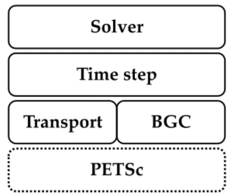
Figure 1.Implementation layers of the Metos3D simulation pack-age (cf. Sect. 5.1).

side of Eq. (6). The line search may also require additional evaluations ofF. Taken together, the overall number of inner iterations plus the overall number of evaluations for the line search determine the number of evaluations ofF necessary for this method, which may then be compared to the number of model years needed for the spin-up.

5 Software description

Our software is divided into four repositories, namely

metos3d, model, data and simpack. The first

com-prises the installation scripts, the second the biogeochemical model source codes and the third all data preparation scripts as well as the data themselves. The last repository contains the simulation package, i.e., the transport driver, which is im-plemented in C and based upon the PETSc library. While we have often used 1-indexed arrays within this text for conve-nience, within the source code C arrays are 0-indexed and Fortran arrays are 1-indexed. All data files are in PETSc for-mat.

5.1 Implementation structure

The implementation of the simulation package is structured in layers as is shown in Fig. 1. The layers are organized hi-erarchically; i.e., each layer provides routines for the layers above. The foundation of the implementation is the PETSc library with its data types and the implementation of the Newton–Krylov solver.

Thebgcmodel layer initializes tracer vectors, parameters and boundary and domain data. It is responsible for the in-terpolation of forcing data and the evaluation of the biogeo-chemical model (cf. Sect. 5.3). Thetransportlayer is respon-sible for reading in the transport matrices, interpolating them to the current time step and applying them to the tracer vec-tors. The main integration routineφ(cf. Algorithms 1 and 2) is located at thetime steppinglayer. On top resides thesolver

(6)

Algorithm 1:Phi(φ)

Input : initial condition:(t0,y0), time step:∆t, number of time steps:nt, implicit matrices:Aimp, explicit matrices:Aexp,

parameters:u∈Rm_{, boundary data:}_b_{, domain data:}_d

Output: final state:yout

1 yin=y0; 2 forj= 1, . . . , ntdo

3 tj= mod (t0+ (j−1) ∆t,1.0);

4 yout=PhiStep(tj,∆t,Aimp,Aexp,yin,u,b,d);

5 yin=yout;

6 end

Algorithm 2:PhiStep(ϕj)

Input : point in time:tj, time step:∆t, implicit matrices:Aimp, explicit matrices:Aexp, current state:yin, parameters:u∈Rm_,

boundary data:b, domain data:d

Output: next state:yout

1 q=BGCStep(tj,∆t,yin,u,b,d);

2 yw=TransportStep(tj,Aexp,yin);

3 yw=yw+q;

4 yout=TransportStep(tj,Aimp,yw);

A call graph for the computation of a steady annual cycle is shown in Fig. 2. Note that loops are not explicitly shown therein. Calls to initialization and finalization routines are gathered at the beginning and end of a simulation run. The former are responsible for memory allocation and storage of data used at run time. The latter are employed to free memory and delete all vectors and matrices.

The dimensions of the used vectors and matrices depend on the underlying geometry (cf. Sect. 5.2). The distribution of the work load for a parallel run is determined during ini-tialization of the work load (cf. Sect. 5.5).

5.2 Geometry information and data alignment

Geometry information is provided as a 2-D land–sea mask plus a designation of the number of vertical layers, i.e., the depth of the different water columns (orprofiles; cf. Fig. 3). This can be understood as a sparse representation of a land– sea cuboid including only wet grid boxes. Hence, the length nxof a single tracer vector (at fixed time) is the sum of the

lengths of all profiles, i.e.,

nx= np X

k=1

nx,k,

where np is the total number of profiles in the ocean and

(nx,k) np

k=1the set of profile lengths. Each profile corresponds

to a horizontal grid point. Due to the locally varying ocean depth, the profile lengths depend on the horizontal coordi-nate, i.e., on the indexk.

We denote byyi,k∈Rnx,k the values of theith tracer

cor-responding to thekth profile at a fixed time step. Then the vector ofalltracers at a fixed time, here denoted byy omit-ting the time index, can be represented in two ways: either by

Main

InitWithFilePath

GeometryInit

LoadInit

BGCInit

TransportInit

TimeStepInit

SolverInit

Solver

TimeStepPhi

TimeStepPhiStep

BGCStep

TransportStep

Final

SolverFinal

TimeStepFinal

TransportFinal

BGCFinal

LoadFinal

GeometryFinal

(7)

1 16 32 48 64 80 96 112 128 Longitudinal grid

1 16 32 48 64

Latitudinal

g

rid

0 5 10 15

Figure 3.Land–sea mask (geometric data) of the used numerical model. Shown are the number of layers per grid point. Note that the Arctic has been filled in.

firstcollecting all profiles for each tracer andthen concate-nating all tracers, namely,

y=h(y1,k) np

k=1. . . (yn,k) np

k=1

i

, (9)

or vice versa, i.e., y=((yi,k)

ny

i=1) np

k=1. (10)

In order to multiply matrices by tracer vectors, the first vari-ant is preferable. In order to evaluate a water-column-based biogeochemical model, the second one is appropriate.

As a result, all tracers need to be copied from representa-tion Eqs. (9) to (10) after a transport step. After evaluarepresenta-tion of the biogeochemical model we reverse the alignment for the next transport step.

The situation is similar for domain data. Again, we group all domain data profiles by their profile indexk, i.e., h

(d1,k) np

k=1. . . (dnd,k)

np

k=1

i

−→((di,k)n_i₌d₁) np

k=1,

wheredi,kdenotes a single domain data profile. However, no

reverse copying is required here.

Boundary data have to be treated in a slightly different way. Here we align boundary values, which are associated with the surface of one water column each,

h (b1,k)

np

k=1. . . (bnb,k)

np

k=1

i

−→((bi,k)ni=b1) np

k=1,

wherebi,kdenotes a single boundary data value as opposed

to a whole profile. As with domain data, no reverse copying is required.

5.3 Biogeochemical model interface

One of our main objectives in this work is to specify a general coupling interface between the transport induced by ocean circulation and the biogeochemical tracer model. We wish to provide a method to couple any biogeochemical model im-plementation using any number of tracers, parameters and

boundary and domain data to the software that computes the ocean transport. Despite the fact that we consider offline sim-ulation using transport matrices in this paper only, the inter-face shall not be restricted to this case. This coupling shall furthermore fit into an optimization context, and it shall be compatible with algorithmic differentiation techniques (cf. Sect. 7).

The only restriction we make for the tracer model is that it operates on each single water column (or profile) sepa-rately. This means that information on exactly one profile is exchanged via the coupling interface. For models that require information on other profiles (e.g., in the horizontal vicinity) for internal computations, a redefinition of the interface and some internal changes would be necessary. In fact, most of the relevant non-local biogeochemical processes take place within a water column (cf. Evans and Garçon, 1997).

The evaluation of a water-column-based biogeochemical model for any fixed timet consists of separate model evalu-ations for each profile (corresponding to a horizontal spatial coordinate), i.e., for profile indexk:

1t (q_i(t, (y_i,k)n_i₌y₁,u, (bi,k)n_i₌b₁, (di,k)n_i₌d₁)) ny

i=1. (11)

Here,(yi,k) ny

i₌1is an input array ofnytracer profiles

accord-ing to Eq. (10), each with a length or depth ofnx,k. The

vec-toru contains nu parameters. Boundary data (bi,k)ni=b1 are

given as a vector ofnbvalues, and domain data(di,k)n_i₌d₁as

an input array ofndprofiles. Results of the biogeochemical

model are stored in the output array (q_i,k)n_i₌y₁, which also consists ofnyprofiles.

Formally speaking this tracer model is scaled from the out-side by the (ocean circulation) time step. However, we have integrated1t into the interface as a concession to the com-mon practice of refining the time step within the tracer model implementation (cf. Kriest et al., 2010). As a consequence, the responsibility for scaling results before returning them to the transport driver software rests with the model imple-menter.

Listing 1 shows a realization of the biogeochemical model interface in a Fortran 95 subroutine called metos3dbgc. The arguments are grouped by data type. The list begins with variables of the type integer, i.e.,ny,nx,k, nu, nb and

nd. These are followed by real*8(double precision)

ar-guments, i.e.,1t,q,tj,y,u,bandd. For clarity we have

omitted the profile indexkand the time indexj in our nota-tion. Moreover, we have useddtas a textual representation of1t.

A model initialization and finalization interface is also specified. The former is namedmetos3dbgcinitand the lattermetos3dbgcfinal. These routines are called at the beginning of each model year, i.e., att0, and after the last

(8)

subroutine metos3dbgc(ny, nx, nu, nb, nd, dt, q, t, y, u, b, d)

integer :: ny, nx, nu, nb, nd

real*8 :: dt, q(nx, ny), t, y(nx, ny), u(nu), b(nb), d(nx, nd)

end subroutine

Listing 1.Fortran 95 implementation of the coupling interface for biogeochemical models.

5.4 Interpolation

Transport matrices as well as boundary and domain data vec-tors are provided as sets of files. The number of files in each set is arbitrary, although most of the data we use in this work represent a monthly mean.

However, time step counts per model year are generally much higher than the number of available data files. For this reason matrices and vectors are linearly interpolated to the current time step during iteration. All files of a specific data set are interpreted as averages of the time intervals they rep-resent. We therefore interpolate between the centers of as-sociated intervals. The appropriate weights and indices are computed on the fly using Algorithm 4.

With regard to boundary and domain forcing, we denote data files by ((bi,j)

nb,i

j=1) nb

i=1 and((di,j) nd,i

j=1) nd

i=1. Here,nb is

the number of distinct boundary data sets, and nb,i is the

number of data files provided for theith set. In the same way, nddenotes the number of domain data sets andnd,ithe

num-ber of data files of a particular set.

For every indexiand its corresponding boundary data set (bi,j)n_jb,i₌₁we compute the appropriate weights α,β as well

as indicesjα,jβand then form a linear combination bi =αbi,jα+βbi,jβ.

The same applies to domain data; i.e., for every domain data set(di,j)

nd,i

j=1, we compute

di =αdi,jα+βdi,jβ.

We use PETSc routines VecCopy, VecScale and

VecAXPYfor this process.

With regard to transport we have (Aimp,j) nimp

j=1 and

(Aexp,j) nexp

j=1 as data files, wherenimp andnexp specify the

number of implicit and explicit matrix files, respectively. Analogous to the interpolation of vectors, we first interpo-late all user-provided matrices to the current point in timetj;

i.e., we assemble A₌αAjα+βAjβ

using the appropriateα,βandjα,jβ. We use the matrix

vari-antsMatCopy,MatScaleandMatAXPYfor this purpose.

The technical details of this process have been discussed in depth in Siewertsen et al. (2013).

To avoid redundant storing we do not assemble both (block-diagonal) system matrices during simulation. We use

the matrices provided to build just one block for each matrix type instead. The transport step is then applied as a loop over individual tracer vectors.

Unlike vector interpolation and vector operations in gen-eral, each matrix operation has a significant impact on com-putational time. In Sect. 6.2 we will present results from pro-filing experiments showing detailed information on the time usage of each operation.

5.5 Load balancing for spatial parallelization

For spatial parallelization, the discrete tracer vectors have to be distributed to the available processes. Since biogeochem-ical models operate on whole water columns, profiles can-not be split without message passing. But due to the locally varying ocean depth, a tracer vector is a collection of profiles withdifferentlengths. Thus a load balancing that takes into account only the number of profiles, but not their respective length, would be sub-optimal.

The PETSc library provides no load balancing algorithm suitable for this case. We therefore use an approach that was inspired by the idea of space filling curves presented by Zum-busch (1999).

For each profile we compute its “computational weight”, i.e., its mid, in relation to the overall computational effort, i.e., the vector length. We then project this ratio to the avail-able number of processes; i.e., we round this figure down to an integer and use the result as the index of the process the profile belongs to. By using this information the profiles can then be assigned consecutively to the processes involved.

For 0-indexed arrays this calculation is described by Algo-rithm 3. Its theoretical and actual performance is discussed in Sect. 6.3, where a comparison between Metos3D and the TMM framework is shown.

6 Results

(9)

Algorithm 3:Load balancing

Input : vector length:nx, number of profiles:np, profile lengths:(nx,k)np

k=1, number of processes:N

Output: profiles per process:(np,i)N i=1

1 w= 0; 2 np,1...N= 0; 3 fork= 1, . . . , npdo

4 i= floor(((w+ 0.5∗nx,k)/ny)∗N); 5 np,i=np,i+ 1;

6 w=w+nx,k; 7 end

Algorithm 4:Interpolation

Input : point in time:t∈_[0_,_1[, number of data points:ndata

Output: weights:α, β, indices:jα, jβ

1 w=t∗_n_data_{+ 0}_.₅_; 2 β= mod(w,1.0);

3 jβ= mod(floor(w), ndata);

4 α= (1.0−β);

5 jα= mod(floor(w) +ndata−1, ndata);

In a second step we have performed speed-up tests to an-alyze the load distribution implemented in our software and compared it with the TMM framework. We will also investi-gate the convergence control settings of the Newton–Krylov solver and examine the solver’s behavior within parameter bounds.

The experimental setup is described in Appendix A in more detail.

6.1 Solver

We begin our verification by computing a steady annual cycle for every model, using both solvers. When using the spin-up we set no tolerance and let the solver iterate for 10 000 model years. The Newton approach is set to a line search variant and the Krylov subspace solver to GMRES. All other settings are left at default, so overall absolute tolerance is at 10−8and the maximum number of inner iterations is 10 000.

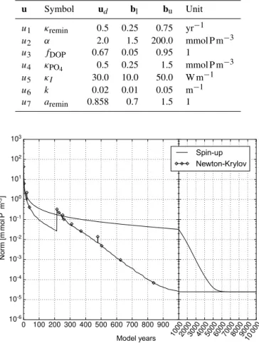
The parameter values used for the MITgcm-PO4-DOP model are listed in Table 2 under the heading ud. Table 3

lists the parameter values used for the N, N-DOP, NP-DOP, NPZ-DOP, NPZD-DOP model hierarchy. If not stated other-wise the initial value is set to 2.17 m mol P m−3_{for N or PO}

4

and 0.0001 m mol P m−3_{for all other tracers.}

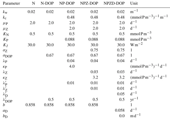
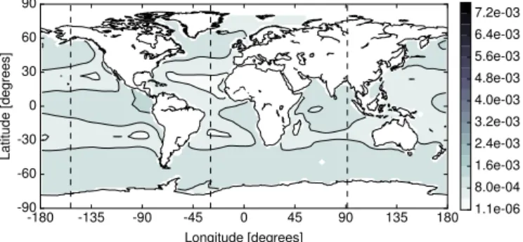
A comparison of convergence towards a steady annual cycle for both solvers, applied to the MITgcm-PO4-DOP model, is shown in Fig. 4. We observe that both solvers reach the same difference between consecutive iterations at the end. Table 4 shows the differences between both solu-tions in Euclidean and volume-weighted norms; cf. Eq. (4). Figure 5 depicts the difference between both solutions for

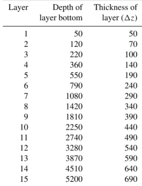
Table 1.Vertical layers of the numerical model, in meters.

Layer Depth of Thickness of layer bottom layer (1z)

1 50 50

2 120 70

3 220 100

4 360 140

5 550 190

6 790 240

7 1080 290

8 1420 340

9 1810 390

10 2250 440

11 2740 490

12 3280 540

13 3870 590

14 4510 640

15 5200 690

one tracer at the surface layer. Except for numerical error, both solvers obviously compute the same solution.

Figures 6 and 7 show the convergence behavior of both solvers for the N and N-DOP models, respectively. Again, both solvers end with approximately the same accuracy and produce similar results. This impression is confirmed by an inspection of Figs. 8 and 9 as well as Table 4.

(10)

re-Table 2.Parameters implemented in the MITgcm-PO4-DOP model. Specified are the location within the parameter vector, the symbol used by Dutkiewicz et al. (2005) and the value used for the com-putation of the reference solution (ud). Shown are furthermore the

lower (bl) and upper (bu) boundaries used for the parameter

sam-ples experiment.

u Symbol ud bl bu Unit

u1 κremin 0.5 0.25 0.75 yr−1

u2 α 2.0 1.5 200.0 mmol P m−3

u3 fDOP 0.67 0.05 0.95 1

u4 κPO4 0.5 0.25 1.5 mmol P m−

3

u5 κI 30.0 10.0 50.0 W m−1

u6 k 0.02 0.01 0.05 m−1

u7 aremin 0.858 0.7 1.5 1

0 100 200 300 400 500 600 700 800 900 10-6

10-5 10-4 10-3 10-2 10-1 100 101 102 103

N

or

m

[m

m

ol

P

m

]

-3

100020003000400050006000700080009000 10

000

Model years

Spin-up Newton-Krylov

Figure 4.MITgcm-PO4-DOP model: convergence towards an an-nual cycle. Spin-up: norm of the difference between initial states of consecutive model years (solid line). Newton–Krylov: residual norm at a Newton step (diamond) and norm of the GMRES residual during solving (solid line in-between).

veals a peak every 30 model years, which results from the settings of the inner solver, where GMRES is set to perform a restart every 30 years. This option is chosen to reduce the internal storage requirement, but may lead to stagnation for indefinite matrices; cf. Saad (2003, Sect. 6.5.6). It is likely that the Jacobian at some Newton step will become indefi-nite, and thus we assume that this is the case here. Figure 11 and Table 4 do not indicate any influence on the solution, however.

For the NPZ-DOP or NPZD-DOP model, the Newton solver shows a different behavior. For both models the solver does not converge if default settings are used, as depicted in Figs. 12 (top) and 13 (top). Reduction of the residual per step is quite low, which results in a huge number of iterations. In this case the solver was stopped after 50 iterations (the

-180 -135 -90 -45 0 45 90 135 180 Longitude [degrees]

-90 -60 -30 0 30 60 90

L

a

ti

tu

d

e

[d

e

g

re

e

s]

7.3e-06 3.3e-04 6.4e-04 9.6e-04 1.3e-03 1.6e-03 1.9e-03 2.2e-03 2.6e-03

Figure 5.MITgcm-PO4-DOP model. Difference between the phos-phate concentration of the spin-up and the Newton solution at the first layer (0–50 m) in the Euclidean norm. Units are mmol P m−3.

default setting), which is quite high for Newton’s method. This behavior was caused by the fact that convergence of this method – even in its so-called globalized or damped ver-sion used here – at times still depends on the initial guess y0. We therefore used a different one, which was success-ful with the NPZD-DOP model; see Fig. 13 (middle). With the NPZ-DOP model, this procedure still did not work; see Fig. 12 (middle).

However, the result of a second and much easier way to achieve convergence can be seen in Figs. 12 (top) and 13 (top). If the last Newton iteration step did not lead to a big reduction of the residual, which was obviously the case here, the stopping criterion Eq. (8) for the inner iterations of the Newton solver becomes less restrictive. If this criterion is sharpened, the number of inner iterations increases and thus the accuracy of the Newton direction improves. This some-what contradicts the idea formulated in Eisenstat and Walker (1996). Sharpening can easily be achieved by decreasingγ, in this case toγ₌0.3. This tuning led to convergence; see Figs. 12 (bottom) and 13 (bottom). When using these set-tings the same solutions are obtained as with the spin-up, if numerical errors are neglected (see Figs. 14 and 15). This re-sult is confirmed by evaluating the differences in the norm; see Table 4.

It can be observed that as a rule the Newton–Krylov solver does not reach default tolerance within the last Newton step and iterates unnecessarily for 10 000 model years. From now on we will therefore limit the inner Krylov iterations to 200. For our next investigations using the MITgcm-PO4-DOP model we will alter the convergence settings as well to get rid of the over-solving observed before. More detailed exper-iments on this subject are presented in Sect. 6.4.

6.2 Profiling

(11)

Table 3.Parameter values used for the solver experiments with the N, N-DOP, NP-DOP, NPZ-DOP and NPZD-DOP model hierarchy.

Parameter N N-DOP NP-DOP NPZ-DOP NPZD-DOP Unit

kw 0.02 0.02 0.02 0.02 0.02 m−1

kc 0.48 0.48 0.48 (mmol P m−3)−1m−1

µP 2.0 2.0 2.0 2.0 2.0 d−1

µZ 2.0 2.0 2.0 d−1

KN 0.5 0.5 0.5 0.5 0.5 mmol P m−3

KP 0.088 0.088 0.088 mmol P m−3

KI 30.0 30.0 30.0 30.0 30.0 W m−2

σZ 0.75 0.75 1

σDOP 0.67 0.67 0.67 0.67 1

λP 0.04 0.04 0.04 d−1

κP 4.0 (mmol P m−3)−1d−1

λZ 0.03 0.03 d−1

κZ 3.2 3.2 (mmol P m−3)−1d−1

λ′_P 0.01 0.01 0.01 d−1

λ′_Z 0.01 0.01 d−1

λ′_D 0.05 d−1

λ′_DOP 0.5 0.5 0.5 0.5 yr−1

b 0.858 0.858 0.858 0.858 1

aD 0.058 d−1

bD 0.0 m d−1

Table 4.Difference in the Euclidean(k · k2) and volume-weighted (_k·k2_,V; cf. Eq. 4) norms between the spin-up (y_S) and the Newton (y_N) solution for all models. The total volume of the ocean used here isV _≈1.174_×1018m3. Solutions for models NPZ-DOP and NPZD-DOP were produced by experiments with altered inner ac-curacy or initial value, respectively.

Model ky_S−yNk2 ky_S−yNk2,V

MITgcm-PO4-DOP 1.460e-01 7.473e+05

N 4.640e-01 2.756e+06

N-DOP 2.421e-01 1.199e+06 NP-DOP 7.013e-02 3.633e+05 NPZ-DOP 1.421e-02 8.514e+04 NPZD-DOP 3.750e-02 2.062e+05

For this purpose we perform aprofiledsequential run for each model, iterating for 10 model years. An analysis of our profiling results is shown in Figs. 16–18. When using the MITgcm-PO4-DOP model, for instance, the biogeochemi-cal model takes up 40 % of computational time. Interpo-lation of matrices (MatCopy,MatScaleandMatAXPY) amounts to approximately one-third. Matrix–vector multipli-cation (MatMult) takes up a quarter of all computations and all other operations amount to 0.5 %.

Our data also suggest that the greater the number of tracers involved, the more dominant matrix–vector multiplication becomes. TheMatMultoperation takes up 19.8 % of com-putational time for the N model, but 56.7 % for the NPZD-DOP model. In Table 5 the absolute timings and the

comput-0 100 200 300 400 500 600 700 800 900 10-6

10-5 10-4 10-3 10-2 10-1 100 101 102 103

N

or

m

[m

m

ol

P

m

]

-3

100020003000400050006000700080009000 10000

Model years

Figure 6.N model: convergence towards an annual cycle using spin-up and the Newton–Krylov solver.

ing time per tracer vs. the number of tracers are shown. The figures confirm the growing dominance of the matrix–vector multiplication. The computing time per tracer converges to-wards 22 s, which is the absolute time spent by theMatMult

(12)

Table 5.Minimum, maximum, average and standard deviations from computational time for 1 model year as well as the computing time per tracer are shown. All computations were performed on a single-core Intel Xeon®E5-2670 CPU at 2.6 GHz.

Min Max Avg SD Min per tracer

N 112.53 s 112.87 s 112.79 s 0.09 112.53 s N-DOP 142.96 s 143.30 s 143.12 s 0.11 71.48 s NP-DOP 160.32 s 161.28 s 160.86 s 0.30 53.44 s NPZ-DOP 185.46 s 185.70 s 185.53 s 0.07 46.37 s NPZD-DOP 193.99 s 194.63 s 194.09 s 0.19 38.80 s

0 100 200 300 400 500 600 700 800 900 10-6

10-5 10-4 10-3 10-2 10-1 100 101 102 103

N

or

m

[m

m

ol

P

m

]

-3

100020003000400050006000700080009000 10 000

Model years

Figure 7.N-DOP model: convergence towards an annual cycle us-ing a spin-up and a Newton–Krylov solver.

Siewertsen et al. (cf. 2013) also made use of this profiling capacity when porting the software to an NVIDIA graphics processing unit (GPU). The authors investigated the impact of the accelerator’s hardware on the simulation of biogeo-chemical models. Their work comprises a detailed discussion of peak performance and memory bandwidth and includes a counting of floating point operations.

6.3 Speed-up

In this section we will investigate in detail the performance of the load balancing algorithm and compare our results with the scalability provided by the TMM framework. We com-pile both drivers using the same biogeochemical model. We choose the MITgcm-PO4-DOP model using the same time step, initial condition as well as boundary and domain data.

Our tests are run on hardware located at the computing center of Kiel University: an Intel®Sandy Bridge EP archi-tecture with Intel Xeon® E5-2670 CPUs that consist of 16 cores running at 2.6 GHz. We perform 10 tests for our imple-mentation, using 1 to 256 cores.

Each test consists of a simulation run of 3 model years, where each year is timed separately. For the TMM

frame--180 -135 -90 -45 0 45 90 135 180 Longitude [degrees]

-90 -60 -30 0 30 60 90

L

a

ti

tu

d

e

[d

e

g

re

e

s]

8.3e-07 2.3e-03 4.6e-03 7.0e-03 9.3e-03 1.2e-02 1.4e-02 1.6e-02 1.9e-02

Figure 8.N model: difference between the phosphate concentration of the spin-up and the Newton solution at the first layer (0–50 m) in the Euclidean norm. Units are mmol P m−3.

work we use 1 to 192 cores and run five tests on each core. We use the given output here, which shows the timing for one whole run.

To calculate speed-up and efficiency we use the minimum timings for a specific number of cores. All timings are re-lated to the timing of a sequential run. For a set of compu-tational times(ti)N_i₌₁measured during our experiments, with

N₌192 orN₌256, respectively, we calculate speed-up as si =t1/ti and efficiency asei =100×si/ i.

To investigate the load distribution implemented by us (cf. Sect. 5.5), we compute the best ratio possible between a se-quential and parallel run. Using Algorithm 3 we first com-pute the load distribution for all numbers of processes, i.e., i₌1, . . .,260, and then retrieve the maximum (local) length ni,max. To calculate speed-up we divide the vector length by

this value, i.e.,si=ny/ni,max, and to calculate efficiency we

again useei=100×si/ i.

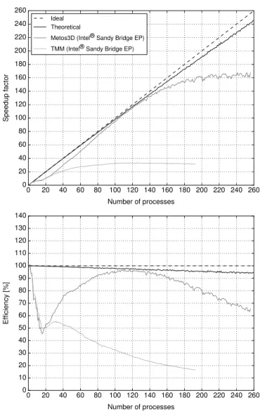
Figure 19 depicts ideal, theoretical and actual data for speed-up and efficiency. Here, the term “ideal” refers to a perfectly parallelizable program and a perfect hardware with no delay in memory access or communication. Regarding the load distribution implemented by us, a good (theoretical) per-formance can be observed over the whole range of processes. This refers again to a perfect hardware except that we dis-tribute a collection of profiles of different lengths here.

(13)

-180 -135 -90 -45 0 45 90 135 180 Longitude [degrees]

-90 -60 -30 0 30 60 90

L

a

ti

tu

d

e

[d

e

g

re

e

s]

1.1e-06 8.0e-04 1.6e-03 2.4e-03 3.2e-03 4.0e-03 4.8e-03 5.6e-03 6.4e-03 7.2e-03

Figure 9. N-DOP model: difference between the phosphate con-centration of the spin-up and the Newton solution at the first layer (0–50 m) in the Euclidean norm. Units are mmol P m−3.

0 100 200 300 400 500 600 700 800 900 10-6

10-5 10-4 10-3 10-2 10-1 100 101 102 103

N

or

m

[m

m

ol

P

m

]

-3

100020003000400050006000700080009000 10 000

Model years

Figure 10.NP-DOP model. Convergence towards an annual cycle using a spin-up and a Newton–Krylov solver.

in this range and speed-up nearly corresponds to the num-ber of processes. In fact speed-up may rise still further up to slightly over 160, but a minimum of 200 processes are re-quired to achieve this.

In comparison, the scalability of the TMM framework is not optimal. Efficiency drops off immediately and speed-up never rises above 40. For 120 cores and above, Metos3D is at least 4 times faster. Interestingly, for low numbers of pro-cesses a significant drop in performance can be observed for both drivers. The implications of this are discussed briefly in Sect. 7. We did not investigate this effect any further, how-ever, since the results presented here already provide a good guideline.

6.4 Convergence control

After this basic verification and the review of some tech-nical aspects of our implementation, we will now investi-gate those settings that control convergence of the Newton– Krylov solver. Once again we use only the

MITgcm-PO4--180 -135 -90 -45 0 45 90 135 180 Longitude [degrees]

-90 -60 -30 0 30 60 90

L

a

ti

tu

d

e

[d

e

g

re

e

s]

2.4e-06 1.1e-04 2.3e-04 3.4e-04 4.5e-04 5.6e-04 6.7e-04 7.8e-04 9.0e-04 1.0e-03

Figure 11.NP-DOP model: difference between the phosphate con-centration of the spin-up and the Newton solution at the first layer (0–50 m) in the Euclidean norm. Units are mmol P m−3.

DOP model. Our intention here is to eliminate the over-solving we observed during the first 200 iterations as shown in Fig. 4. This effect occurs if the accuracy of the inner solver is significantly higher than the resulting Newton residual (cf. Eisenstat and Walker, 1996). The relation between these two is controlled by the parametersγand theαused in Eq. (8).

To investigate the influence of these parameters on con-vergence, we compute the reference solution described in Sect. 6.1 using different values of γ and α. We set over-all tolerance to the difference measured between consecutive states after 3000 model years of spin-up, i.e., approximately 9.0×10−4.γ is varied from 0.5 to 1.0 in steps of 0.1 andα from 1.1 to 1.6, also in steps of 0.1. This makes for a total of 36 model evaluations.

Figure 20 depicts the number of model years and New-ton steps required as a function ofγ andα. We observe that the overall number of years decreases as the two parameters tend towards 1.0 and 1.1, respectively. In contrast, the num-ber of Newton steps increases; i.e., the Newton residual is computed more often and the inner steps become shorter.

Consequently, since the computation of one residual is negligible in comparison to the simulation of 1 model year, we focus on decreasing the overall number of model years. A detailed inspection of the results reveals that forγ₌1.0 andα₌1.2 the solver reaches the tolerance set above after approximately 450 model years, which is significantly less than the 600 years needed when using the default settings.

We therefore use these values for our next experiment. 6.5 Parameter samples

(14)

0 100 200 300 400 500 600 700 800 900 10-6 10-5 10-4 10-3 10-2 10-1 100 101 102 103 N or m [m m ol P m ] 3-100020003000400050006000700080009000 10 000 Model years Spin-up Newton-Krylov

0 100 200 300 400 500 600 700 800 900 10-6 10-5 10-4 10-3 10-2 10-1 100 101 102 103 N or m [m m ol P m ]

3-100020003000400050006000700080009000₁₀000

Model years

Figure 12.NPZ-DOP model. Convergence towards an annual cycle using a spin-up and a Newton–Krylov solver. Top: default Newton– Krylov setting. Middle: initial value altered to 0.5425 mmol P m−3 for all tracers. Bottom: inner accuracy altered toγ=0.3.

0 100 200 300 400 500 600 700 800 900 10-6 10-5 10-4 10-3 10-2 10-1 100 101 102 103 N or m [m m ol P m ] 3

-100020003000400050006000700080009000₁₀000

Model years

(15)

-180 -135 -90 -45 0 45 90 135 180 Longitude [degrees] -90 -60 -30 0 30 60 90 L a ti tu d e [d e g re e s] 7.9e-08 7.2e-05 1.4e-04 2.2e-04 2.9e-04 3.6e-04 4.3e-04 5.0e-04 5.8e-04 6.5e-04

Figure 14. NPZ-DOP model: difference between the phosphate concentration of the spin-up and the Newton solution at the first layer (0–50 m) in the Euclidean norm. Units are mmol P m−3.

-180 -135 -90 -45 0 45 90 135 180 Longitude [degrees] -90 -60 -30 0 30 60 90 L a ti tu d e [d e g re e s] 3.1e-06 1.6e-04 3.1e-04 4.7e-04 6.2e-04 7.8e-04 9.4e-04 1.1e-03 1.2e-03

Figure 15. NPZD-DOP model: difference between the phosphate concentration of the spin-up and the Newton solution at the first layer (0–50 m) in the Euclidean norm. Units are mmol P m−3.

As before we set overall tolerance to a value comparable to 3000 spin-up iterations and let the Newton solver compute a solution for each parameter sample.

Figure 21 shows histograms of the total number of model years or Newton steps required to solve the model equations. We observe that most computations converge after 400 to 550 model years and require 10 to 30 Newton steps. Interestingly, there is a high peak around 15 and a smaller one around 12 for the Newton method. We also find some outliers in both graphs. Nevertheless, all model evaluations we started con-verged towards a solution within the desired tolerance.

7 Conclusions

We designed and implemented a simulation framework for the computation of steady annual cycles for a generalized class of marine ecosystem models in 3-D, driven by trans-port matrices pre-computed in an offline mode. Our frame-work allows computation of steady cycles by spin-up or by a globalized Newton method. The software has been realized as open-source code throughout.

We also introduced a software interface for water-column-based biogeochemical models. We demonstrated the applica-bility and flexiapplica-bility of this interface by coupling the

biogeo-BGCStep 40.4 % MatCopy 13.1 % MatScale 7.9 % MatAXPY 15.1 % MatMult 23.1 % Other 0.5 % BGCStep 19.0 % MatCopy 22.2 %

MatScale _{13.3 %}

MatAXPY 25.4 % MatMult 19.8 % Other 0.4 %

Figure 16.Distribution of computational time among main opera-tions during integration of 1 model year. Left: MITgcm-PO4-DOP model. Right: N model.

BGCStep 19.8 % MatCopy 17.6 % MatScale 10.6 % MatAXPY 20.3 % MatMult 31.0 % Other 0.6 % BGCStep 15.1 % MatCopy 15.6 % MatScale 9.4 %

MatAXPY 18.0 %

MatMult 41.0 %

Other 0.9 %

Figure 17.Distribution of computational time among main opera-tions during integration of 1 model year. Left: N-DOP model. Right: NP-DOP model.

chemical component used in the MITgcm general circulation model to the simulation framework. To test the general us-ability of the interface we then coupled our own implemen-tations of five different biogeochemical models of varying complexity (already used in Kriest et al., 2010) to the frame-work. The source code of these models is also available as part of the software package, and may serve as a template for the implementation or adaption of other models.

We implemented a transient solver based on the transport matrix approach, where all matrix operations and evaluations of biogeochemical models are performed by spatial paral-lelization via MPI using the PETSc library. The transport matrices needed for this process are available directly and require no pre-processing.

(16)

BGCStep 14.1 % MatCopy 13.5 % MatScale 8.2 % MatAXPY 15.6 % MatMult 47.5 % Other 1.0 % BGCStep 6.5 % MatCopy 12.9 % MatScale 7.8 % MatAXPY 14.9 % MatMult 56.7 % Other 1.2 %

Figure 18. Distribution of computational time among main oper-ations during integration of 1 model year. Left: NPZ-DOP model. Right: NPZD-DOP model.

0 20 40 60 80 100 120 140 160 180 200 220 240 260 Number of processes

0 20 40 60 80 100 120 140 160 180 200 220 240 260 S p e e d u p fa ct o r Ideal Theoretical

Metos3D (Intel® Sandy Bridge EP) TMM (Intel® Sandy Bridge EP)

0 20 40 60 80 100 120 140 160 180 200 220 240 260 Number of processes

0 10 20 30 40 50 60 70 80 90 100 110 120 130 140 E ffici e n cy [% ]

Figure 19.MITgcm-PO4-DOP model: ideal and actual speed-up factors and efficiency of parallelized computations. The term “the-oretical” here refers to the use of load distribution as introduced in Sect. 6.3.

With regard to performance, the Newton solver was about 6 times faster for all models. It can be concluded that for complex models the Newton method requires more attention to solver parameter settings, but then is superior to the spin-up, at least when using parameter sets as described above.

Alpha(α)

1.1 1.2 1.3 1.4 1.5 1.6 G am_m a (_γ ) 0.5 0.6 0.7 0.8 0.9 1.0 M o d e l ye a rs 450 500 550 600 650

Alpha(α)

1.1 1.2 1.3 1.4 1.5 1.6 Gamma (_γ ) 0.5 0.6 0.7 0.8 0.9 1.0 N e_w to_n st e_p s 10 12 14 16 18 20

Figure 20.MITgcm-PO4-DOP model: number of model years and Newton steps required for the computation of the annual cycle y(u_d)as a function of different convergence control parametersα andγ (cf. Eq. 8).

In a next step we investigated how performance of the Newton method is influenced by the two solver parameters α, γin Eq. (8), using one model as an example.

(17)

op-300 400 500 600 700 800 900 1000 Model years

0 2 4 6 8 10 12 14 16

O

ccu

rr

e

n

ce

5 10 15 20 25 30 35 40 45

Newton steps 0

2 4 6 8 10 12 14

O

ccu

rr

e

n

ce

Figure 21.Distribution of the number of model years and Newton steps required for the computation of one annual cycle using 100 random parameter samples (cf. Sect. 6.5).

timization, at least for this model, and faster than the usually robust spin-up.

We further analyzed which proportion of computational time is utilized by different parts of our software during sim-ulation of 1 model year. Our experiments showed that with an increase in the number of tracers the matrix–vector op-erations started to dominate the process, thus offering the greatest potential for further performance tuning. This was the case even though the transport operator was the same for every tracer. In contrast, all biogeochemical interactions contained in the nonlinear coupling termsqj, which mostly

are spatially local, become less performance-relevant as the number of tracers increases.

Finally, we implemented a load balancing mechanism that exploits the fact that water columns in the ocean vary in depth, resulting in data vectors of variable length. Using this balancing method, a close to optimal speed-up by spatial

par-allelization was achieved up to the relatively high number of 140 processes. This results in an acceleration factor of 4 com-pared to the TMM framework. The factor increases even to 5 if 200 processes are used. However, here already 20 % of computational resources are wasted.

To summarize, the software framework presented here of-fers high flexibility w.r.t. models and steady cycle solvers. The implemented load balancing scheme results in signif-icant improvement in parallel performance. Especially the applied Newton solver can be tuned to converge for all six biogeochemical models.

8 Code availability

Name of software: Metos3D (Simulation Package v0.3.2) Developer: Jaroslaw Piwonski

Year first available: 2012 Software required: PETSc 3.3 Program language: C, C++, Fortran Size of installation: 1.6 GB

Availability and costs: free software, GPLv3

Software homepage: https://metos3d.github.com/metos3d The toolkit is maintained using distributed revision con-trol systemgit. All source codes are available at GitHub (https://github.com). The current versions ofsimpackand

modelare tagged asv0.3.2. The data repository is tagged

as version v0.2. All experiments presented in this work were carried out using these versions. Associated material is stored in the2016-GMD-Metos3Drepository.

To install the software, users should visit the homepage and follow instructions. Future installations will reflect the state of development at that point of time, but users may still retrieve the versions used in this work by invokinggit

checkout v0.3.2in thesimpackandmodel

(18)

Appendix A: Experimental setup

We assume that all PETSc environment variables have been set, the toolkit has been installed and themetos3d script has been made available as a shell command.

A1 Models

In order to test our interface we couple an N, N-DOP, NP-DOP, NPZ-NP-DOP, NPZD-DOP model hierarchy as well as an implementation of Dutkiewicz et al. (2005)’s original bio-geochemical model. The former has been implemented from scratch for this purpose. The corresponding equations are shown in Appendix B. The latter is the model used for the MIT general circulation model (cf. Marshall et al., 1997, MITgcm) biogeochemistry tutorial. We will denote it as the MITgcm-PO4-DOP model.

For every model implementation that is coupled to the transport driver via the interface a new executable must be compiled. We have established naming conventions for the directory structure so that it fits seamlessly into an automatic compile scheme. We create a folder that is named after the biogeochemical model, for instance MITgcm-PO4-DOP, within themodeldirectory of themodelrepository.

Within this folder the source code file namedmodel.F

is stored. This directory structure is used for all models. Al-though the file suffix used here implies a pre-processed For-tran fixed format, any programming language supported by the PETSc library will be accepted.

To compile all sources (still using the same example) we invoke

$> metos3d simpack MITgcm-PO4-DOP

and obtain an executable named

metos3d-simpack-MITgcm-PO4-DOP.exe

which we will use forallexperiments described below. Specific settings will be provided via option files. A2 Data

All matrices and forcing data used in this work are based on the example material available in Khatiwala (2013). This material originates from MITgcm simulations and requires some post-processing. The corresponding preparation scripts are provided along with the processed data in the data

repository.

The surface grid of the domain used has a longitudinal and latitudinal resolution of 2.8125◦, which produces 128×64 grid points (cf. Fig. 3). Note that the Arctic has been filled in, i.e., set to land. This originates in the data provided at the TMM webpage (cf. Khatiwala, 2013). The depth is divided into 15 vertical layers as described in Table 1. This geometry translates to a (single) tracer vector length ofnx=52749 and

tonp=4448 corresponding profiles. Temporal resolution is

at1t₌1/2880, which is equivalent to an (ocean) time step of 3 h, assuming that 1 year consists of 360 days.

The method of computing photosynthetically available shortwave radiation is the same for all models. It is deduced from insolation, which is computed on the fly using the for-mula of Paltridge and Platt (1976). For this purpose lati-tude and ice cover data are required for the topmost layer, i.e.,nb=2. We use a single latitude file for the former, i.e.,

nb,1=1, and 12 ice cover files for the latter,nb,2=12.

The depths and heights of all vertical layers are required as well, so we havend=2 domain data sets. Each set consists

of only one file, i.e.,nd,1=1 and nd,2=1. This

informa-tion is used to compute the attenuainforma-tion of light by water to determine the fluxes of particulate organic phosphorus and to approximate a derivative with respect to depth. Note that these data sets have to be provided in a specific order, which must correspond to the order used within the model imple-mentation. In addition, 12 implicit transport matrices, i.e., nimp=12, and 12 explicit transport matrices, i.e.,nexp=12,

are provided as mentioned previously. Each simulation starts att0=0 and performsnt =2880 iterations per model year.

Appendix B: Model equations

The N, N-DOP, NP-DOP, NPZ-DOP and NPZD-DOP model hierarchy presented here is based on the descriptions used by Kriest et al. (2010). All parameters introduced are shown in Table 3.

B1 Shortwave radiation

As mentioned in Sect. A2, shortwave radiation for the top-mostlayer is deduced from insolation, which is computed on the fly using the formula of Paltridge and Platt (1976). For this purpose latitudeφand ice coverσice data are required.

We denote the computed value byISWR=ISWR(φ, σice). For

all lower layers, data on depth(zj)n_jx₌₁and height(dzj)n_jx₌₁

are required. Attenuation by water is described by the coef-ficientkwand attenuation by phytoplankton (chlorophyll) by

kc.

B1.1 Implicit phytoplankton

For models N and N-DOP, shortwave radiation is computed

withoutphytoplankton, i.e.,

Ij=ISWR

(

I_j′ j₌1,

I_j′Qj−1

k=1Ik else,

where I_j′ ₌exp(−kwdzj/2), Ij=exp(−kwdzj), and j is

(19)

B1.2 Explicit phytoplankton

For models NP-DOP, NPZ-DOP and NPZD-DOP, shortwave radiation is computedwithphytoplankton included, i.e.,

IP,j=ISWR

(

I_P′_,j j₌1,

I_P′_,jQj−1

k=1IP,k else,

where I_P′_,j₌exp(−(kw+kcyP,j)dzj/2) and IP′,k=

exp(−(kw+kcyP,k)dzk).

B2 N model

The simplest model used here consists of nutrients (N) only, i.e., y₌(y_N). The equation is presented in Table B1. Bio-logical uptake is computed as

fP(yN, I )=µPy∗P

y_N KN+yN

I KI+I

,

where the implicitly prescribed concentration of phyto-plankton is set to y∗_P₌0.0028 mmol P m−3. Note that y∗_P could be a free model parameter as well. However, we stick to this formulation to be consistent with Kriest et al. (2010). The N model introduces nu=5 parameters, with u=(kw, µP, KN, KI, b).

B3 N-DOP model

The N-DOP model consists of nutrients (N) and dissolved organic phosphorus (DOP), i.e.,y₌(yN,yDOP).

Computa-tion of biological uptake remains the same. The equaComputa-tions are shown in Table B2. The N-DOP model introducesnu=7

pa-rameters, withu=(kw, µP, KN, KI, σDOP, λDOP, b).

B4 NP-DOP model

The NP-DOP model consists of nutrients (N), phytoplank-ton (P), and dissolved organic phosphorus (DOP), i.e.,y=

(yN,yP,yDOP). Here nutrient uptake by (explicit)

phyto-plankton is computed as fP(yN,yP, IP)=µPyP

yN

KN+yN

IP

KI+IP

.

Computation of shortwave radiation is altered as well (see Sect. B1.2). In addition, a quadratic loss term for phytoplank-ton is introduced, as is a grazing function

fZ(yP)=µZy∗Z

y2_P K_P2₊y2_P,

where the implicitly prescribed concentration of zoo-plankton is set to y∗_Z₌0.01 mmol P m−3. Again, we stick to this formulation to be consistent with Kriest et al. (2010), though y∗_Z could be a free model parame-ter. The equations are shown in Table B3. The NP-DOP model introduces nu=13 parameters, with u=

(kw, kc, µP, µZ, KN, KP, KI, σDOP, λP, κP, λ′_P, λDOP, b).

B5 NPZ-DOP model

The NPZ-DOP model consists of nutrients (N), phytoplank-ton (P), zooplankphytoplank-ton (Z) and dissolved organic phosphorus (DOP), i.e., y=(yN,yP,yZ,yDOP). The production

func-tion remains the same. For the computafunc-tion of grazing, zoo-plankton is dealt with explicitly, i.e.,

fZ(yP,yZ)=µPyZ

y2_P K_P2₊y2

P

.

The equations are shown in Table B4. The NPZ-DOP model introduces nu=16 parameters, with u₌(kw, kc, µP, µZ, KN, KP, KI, σZ, σDOP, λP, λZ, κZ,

λ′_P, λ′_Z, λ′_DOP, b).

B6 NPZD-DOP model

The NPZD-DOP model consists of nutrients (N), phyto-plankton (P), zoophyto-plankton (Z), detritus (D) and dissolved organic phosphorus (DOP), i.e.,y=(yN,yP,yZ,yD,yDOP).

Most equations are unchanged, except that a depth-dependent linear sinking speed is introduced for detritus. The equations are shown in Table B5. The NPZD-DOP model introduces nu=16 parameters, with u=

(kw, kc, µP, µZ, KN, KP, KI, σZ, σDOP, λP, λZ, κZ, λ′P, λ′Z,