Education
Chapter 10: Mining Genome-Wide Genetic Markers
Xiang Zhang1, Shunping Huang2, Zhaojun Zhang2, Wei Wang3*
1Department of Electrical Engineering and Computer Science, Case Western Reserve University, Ohio, United States of America,2Department of Computer Science, University of North Carolina at Chapel Hill, North Carolina, United States of America,3Department of Computer Science, University of California at Los Angeles, California, United States of America
Abstract: Genome-wide associa-tion study (GWAS) aims to discover genetic factors underlying pheno-typic traits. The large number of genetic factors poses both compu-tational and statistical challenges. Various computational approaches have been developed for large scale GWAS. In this chapter, we will discuss several widely used com-putational approaches in GWAS. The following topics will be cov-ered: (1) An introduction to the background of GWAS. (2) The existing computational approaches that are widely used in GWAS. This will cover single-locus, epistasis detection, and machine learning methods that have been recently developed in biology, statistic, and computer science communities. This part will be the main focus of this chapter. (3) The limitations of current approaches and future di-rections.
This article is part of the ‘‘Transla-tional Bioinformatics’’ collection for
PLOS Computational Biology.
1. Introduction
With the advancement of genotyping technology, genome-wide high-density sin-gle nucleotide polymorphisms (SNPs) of human and other organisms are now available [1,2]. The goal of genome-wide association studies (GWAS) is to seek strong associations between phenotype and genetic variations in a population that represent (genomically proximal) causal genetic effects. As the most abundant source of genetic variation, millions of SNPs have been genotyped across the entire genome. Analyzing such large amount of markers poses great challenges to traditional computational and statistical methods. In this chapter, we introduce the basic concept of genome-wide association study, and discuss recently developed methods for GWAS.
Genome-wide association study is an inter-discipline problem of biology,
statis-tics and computer science [3,4,5,6]. In this section, we will first provide a brief introduction to the necessary biological background. We will then formalize the problem and discuss both traditional and recently developed methods for genome-wide analysis of associations.
A human genome contains over 3 billion DNA base pairs. There are four possible nucleotides at each base in the DNA: adenine (A), guanine (G), thymine (T), and cytosine (C). In some locations in the genome, a genetic variation may be found which involves two or more nucleotides across different individuals. These genetic variations are known as single-nucleotide polymorphism (SNPs), i.e., a variation of a single nucleotide in the DNA sequence. In most cases, there are two possible nucleo-tides for a variant. We denote the more frequent one as ‘‘0’’, and the less frequent one as ‘‘1’’. For bases on autosomal chromosomes, there are two parallel nucle-otides, which leads to three possible combinations, ‘‘00’’, ‘‘01’’ and ‘‘11’’. These genotype combinations are known as ‘‘major homozygous site’’, ‘‘heterozygous site’’ and ‘‘minor heterozygous site’’ re-spectively. These genetic variations con-tribute to the phenotypic differences among the individuals. (A phenotype is the com-posite of an organism’s observable charac-teristics or traits.) Genome-wide association study (GWAS) aims to find strong associa-tions between SNPs and phenotypes across a set of individuals.
More formally, let X~fX1,X2, ,
XNg be the set of N SNPs for M
individuals in the study, and Y be the phenotype of interest. The goal of GWAS
is to find SNPs (markers) in X, that are highly associated with Y. There are several challenging issues that need to be addressed when developing an analytic method for GWAS [7,8].
ScalabilityMost GWAS datasets consist of a large number of SNPs. Therefore the algorithms for GWAS need to be highly scalable. For example, for a typical human GWAS, the dataset may contain up to millions SNPs and involve thousands of individuals. Inefficient methods may con-sume a large amount of computational resources and time to find highly associated SNPs.
Missing markers Even with the
current dense genotyping technique, many genetic variants are still not genotyped. Current methods usually assume genetic linkage to enhance the power. Imputation, which tries to impute the unknown markers by using existing SNPs databases, is another popular approach to handle missing markers. The well known related projects include the International Hap-Map project [9] and the 1000 Genomes Project [10].
Complex traits One approach in
GWAS is to test the association between the trait and each marker in a genome, which is successful in detecting a single gene related disease. However, this ap-proach may have problems in finding markers associated with complex traits. This is because that complex traits are affected by multiple genes, and each gene may only have a weak association with the phenotype. Such markers with low mar-ginal effects are hard to detect by the single-locus methods.
Citation:Zhang X, Huang S, Zhang Z, Wang W (2012) Chapter 10: Mining Genome-Wide Genetic Markers. PLoS Comput Biol 8(12): e1002828. doi:10.1371/journal.pcbi.1002828
Editors:Fran Lewitter, Whitehead Institute, United States of America and Maricel Kann, University of Maryland, Baltimore County, United States of America
PublishedDecember , 2012
Copyright: ß2012 Zhang et al. This is an open-access article distributed under the terms of the Creative Commons Attribution License, which permits unrestricted use, distribution, and reproduction in any medium, provided the original author and source are credited.
Funding:This work was supported by the following grants: NSF IIS-1162369, NSF IIS-0812464, NIH GM076468 and NIH MH090338. The funders had no role in the preparation of the manuscript.
Competing Interests:The authors have declared that no competing interests exist. * E-mail: [email protected]
In the remainder of the chapter, we will first discuss the single-locus methods. We will then study epistasis detection (multi-locus) approaches which are designed for association studies of complex traits. For epistasis detection, we will mainly focus on exact two-locus association mapping methods.
2. Single-Locus Association Mapping
As the rapid development of high-throughput genotyping technology, mil-lions of SNPs are now available for genome-wide association studies. Single-locus association test is a traditional way for association studies. Specifically, for each SNP, a statistical test is performed to evaluate the association between the SNP and the phenotype. A variety of tests can be applied depending on the data types. The phenotype involved in a study can be case-control (binary), quantitative (continuous), or categorical. We categorize the statistical tests based on what kind of phenotypes they can be applied on.
2.1 Problem Formalization
LetfX1, ,XNgbe a set of N SNPs for M individuals and Xn~fXn1, ,XnMg(1ƒnƒN). We use 0, 1, 2 to represent the homozygous major allele, heterozygous allele, and homozygous mi-nor allele respectively. Thus we have that
Xnm[f0,1,2g (1ƒnƒN,1ƒmƒM). Let
Y~fy1, ,yMgbe the phenotype. Note that the values thatYcan take depend on its type.
2.2 Case-Control Phenotype
In a case-control study, the phenotype can be represented as a binary variable with 0 representing controls and 1 repre-senting cases.
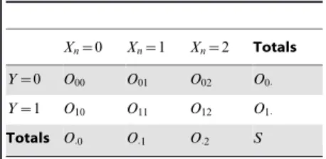
A contingency table records the
frequencies of different events. Table 1 is an example contingency table. For a SNPXnand a phenotypeY, and we use
Oij to denote the number of individuals whoseXnequalsiandYequalsj. Also, we have Oi:~P
j
Oij and O:j~P i
Oij .
The total number of individuals
S~P i,j
Oij .
Many tests can be used to assess the significance of the association between a single SNP and a binary phenotype. The test statistics are usually based on the contingency table. The null hypothesis is that there is no association between the rows and columns of the contingency table.
2.2.1 Pearson’sx2test. Pearson’sx2
test can be used to test a null hypothesis stating that the frequency distribution of certain events observed in a sample is consistent with a particular theoretical distribution [11].
The value of the test statistic is
X2~X i
X
j
(Oij{Eij)2
Eij ,
whereEij~Oi
:O:j
S . The degree of freedom is 2.
2.2.2 G-test. G-test is an approximation of the log-likelihood ratio. The test statistic is
G~2X i
X
j
Oij:ln(
Oij
Eij ),
whereEij~Oi
:O:j S .
The null hypothesis is that the observed frequencies result from random sampling from a distribution with the given expect-ed frequencies. The distribution of G is approximately that of x2, with the same
degree of freedom as in the corresponding
x2test. When applied to a reasonable size
of samples, the G-test and thex2test will
lead to the same conclusions.
2.2.3 Fisher exact test. When the sample size is small, the Fisher exact test is useful to determine the significance of the
association. The p-value of the test is the probability of the contingency table given the fixed margins. The probability of obtaining such values in Table 1 is given by the hypergeometric distribution:
p~
O:0
O00
!
O:1
O01
!
O:2
O02
!
S
O0:
! ~
(O:0!O:1!O:2!)(O0:!O1:!)
S!(O00!O01!O02!O10!O11!O12!)
Most modern statistical packages can calculate the significance of Fisher tests. The actual computation performed by the existing software packages may be different from the exact formulation given above because of the numerical difficulties. A simple, somewhat better computational approach relies on a gamma function or log-gamma function. How to accurately compute hypergeometric and binomial probabilities remains an active research area.
2.2.4 Cochran-Armitage test. For complex traits, contributions to disease risk from SNPs are widely considered to be roughly additive. In other words, the heterozygous alleles will have an inter-mediate risk between two homozygous alleles. Cochran-Armitage test can be used in this case [12,5]. Let the test statistic of U be the following:
U~O1:O0: X2
i~0 i:(O1i
O1: {O0i
O0:)
After substitution, we get
U~S:(O11z2O12{O1::(O:1z2O:2)
The variance of U under the null hypothesis can be computed as
Var(U)~(S
{O1:)O1:
S
½S(O:1z4O:2){(O:1z2O:2)2
Notice that for a large sample sizeS, we have ffiffiffiffiffiffiffiffiffiffiffiU
Var(U)
p *N(0,1), hence U2 Var(U)*x
2 1.
2.2.5 Summary. There is no overall winner of the introduced tests. Cochran-Armitage test may not be the best if the risks are deviated from the additive model. Meanwhile,x2test, G-test, and Fisher exact
test can handle the full range of risks, but they will unavoidably lose some power in the detection of additive ones. Different tests may be applied on the same data to detect different effects.
What to Learn in This Chapter
N
The background of Genome-wide association study (GWAS).N
The existing computational approaches that are widely used in GWAS. This willcover single-locus, epistasis detection, and machine learning methods.N
The limitations of current approaches and future directions.Table 1.Contingency table for a single
SNPXnand a phenotypeY.
Xn~0 Xn~1 Xn~2 Totals
Y~0 O00 O01 O02 O0:
Y~1 O10 O11 O12 O1:
Totals O:0 O:1 O:2 S
2.3 Quantitative Phenotype
In addition to case-control phenotypes, many complex traits are quantitative. This type of study is also often referred to as the quantitative trait locus (QTL) analysis. The standard tools for testing the associ-ation between a single marker and a continuous outcome are analysis of vari-ance (ANOVA) and linear regression.
2.3.1 One-way ANOVA. The F-test in one-way analysis of variance is used to assess whether the expected values of a quantitative variable within several pre-defined groups differ from each other.
For each SNPXn, we can divide all the individuals into three groups according to their genotypes. Let Yi’(i[f0,1,2g) be a
subset of phenotypes of which the individ-uals have the genotypes equal to i. We represent the number of phenotypes inY’i
as Mi, and we haveYi’~fyi1, ,yiMig.
Notice that S2
i~0
Yi’~Y and P2
i~0 Mi~M
The total sum of squares (SST) can be divided into two parts, the between-group sum of squares (SSB) and the within-group sum of squares (SSW):
SST~X M
m~1
(ym{Y)2~
X2
i~0
XMi
m~1
(yim0 {Y)2,
SSB~X
2
i~0
(Yi0{Y)2, and
SSW~SST{SSB~X
2
i~0
XMi
m~1 (yim0 {YY
’
i) 2,
where
Y~ 1
M
XM
m~1
ym and YYi’~ 1 Mi
XMi
m~1 yim’ :
The formula of F-test statistic isF~SSWSSB, and F follows the F-distribution with 2 and S-3 degrees of freedom under the null hypothesis, i.e.,F*F(2,S{3).
2.3.2 Linear regression. In the linear regression model, a least-squares regression line is fit between the phenotype values and the genotype values [11]. For simplicity, we denote the genotypes of a single SNP to bex1,x2, ,xM. Based on the data(x1,y1), ,(xM,yM), we need to fit a line in the form ofY~azbx.
We have the sums of squares as follows:
SSxx~
XM
i~1
(xi{x)2,SSyy~
XM
i~1
(Yi{Y)2,
and SSxy~
XM
i~1
(xi{x)(Yi{Y)
wherex~1 M
PM
i~1
xi and Y~M1 P M
i~1 yi
To achieve least squares, the estimator ofbisSSxy
SSxx. To evaluate the significance of
the obtained model, a hypothesis testing forb~0is then applied.
2.4 Multiple Testing Problem
In a typical GWAS, the test needs to be performed many times. We should pay attention to a statistical issue known as the multiple testing problem. In the remainder of this section, we will discuss the multiple testing problem and how to effectively control error rate in GWAS.
Type 1 error rate, is the possibility that a null hypothesis is rejected when it is actually true. In other words, it is the chance of observing a positive (significant) result even if it is not. If a test is performed multiple times, the overall Type 1 Error rate will increase. This is called the multiple testing problem.
Letabe the type 1 error rate for a statistical test. If the test is performed n times, the experimental-wise error ratea’is given by
a’~1{(1{a)n:
For example, if a~0:05 and n~20, then
a’~1{(1{0:05)20~0:64. In this case, the chance of getting at least one false positive is
64%.
Because of the multiple testing problem, the test result may not be that significant even if its p-value is less than a significant levela. To solve this problem, the nominal p-value need to be corrected/adjusted.
2.5 Family-Wise Error Rate Control
For the single-locus test, we denote the p-value for a association test of a SNPXiand a phenotype Y to be p(Xi,Y), and the corrected p-value to bep’(Xi,Y). Family-wise error rate (FWER), or the experiment-wise error rate, is the probability of at least one false association. We usea’ to denote family-wise error rate, and it is given by
a’~P(rejectH0DH0)~Pðreject at least
one ofHi(1ƒiƒn)DH0Þ,
wherenis the total number of tests andH0is
the hypothesis that all theHi(1ƒiƒn) are true.
Many methods can be used to control FWER. Bonferroni correction is a com-monly used method, in which p-values need to be enlarged to account for the number of comparisons being performed. Permutation test [13] is also widely used to correct for multiple testing in GWAS.
2.5.1 Bonferroni correction. In Bonferroni correction, the p-value of a test is multiplied by the number of tests in the multiple comparison.
p’(Xi,Y)~p(Xi,Y)N
Here the number of tests is the number of SNPsN in a study. Bonferroni correction is a single-step procedure, in which each of the p-values is independently corrected.
2.5.2 Permutation tests. In the permutation test, data are reshuffled. For each permutation, p-values for all the tests are re-calculated, and the minimal p-value is retained. AfterKpermutations, we get totally
Kminimal p-values. The corrected p-value is given by the proportion of minimal p-values which is less than the original p-value.
Let fY1, ,Ykg be the set of K permutations. For each permutation
Yk(1ƒkƒK), the minimal p-value pYk
is given by
pYk~minfp(Xi,Yk)D1ƒiƒng:
Then we have the corrected p-value
p’(Xi,Y)~
#fpYkvp(Xi,Y)D1ƒkƒKg
K :
The permutation method takes advantage of the correlation structure between SNPs. It is less stringent than Bonferroni correction.
2.6 False Discovery Rate Control
False discovery rate (FDR) controls the expected proportion of type 1 error among all significant hypotheses. It is less conservative than the family-wise error rate. For example, if 100 observed results are claimed to be significant, and the FDR is 0.1, then 10 of results are expected to be false discoveries.
One way to control the FDR is as follows [14]. The p-values of SNPs and the phenotype are ranked from smallest to largest. We denote the ordered p-values to bep1, ,pN. Starting from the largest p-value to the smallest, the original p-p-value is multiplied by the total number of SNPs and divided by its rank. For theithp-value
pi, its corrected p-valuepi’ is given by
pi’~pi(N
In this section, we have discussed com-monly used methods in single-locus study, the multiple testing problem and how to control error rate in GWAS. In the next section, we will introduce methods used for two-locus association studies. We will focus on one class work that finds exact solution when searching for SNP-SNP interactions in GWAS.
3. Exact Methods for Two-Locus Association Study
The vast number of SNPs has posed great computational challenge to genome-wide association study. In order to under-stand the underlying biological mecha-nisms of complex phenotype, one needs to consider the joint effect of multiple SNPs simultaneously. Although the idea of studying the association between pheno-type and multiple SNPs is straightforward, the implementation is nontrivial. For a study with totalN SNPs, in order to find the association between nSNPs and the phenotype, a brute-force approach is to exhaustively enumerate all N
n
possible SNP combinations and evaluate their associations with the phenotype. The computational burden imposed by this enormous search space often makes the complete genome-wide association study intractable. Moreover, although permuta-tion test has been considered the gold standard method for multiple testing correction, it will dramatically increase the computational burden because the process needs to be performed for all permuted data.
In this section, we will focus on the recently developed exact method for two-locus epistasis detection. Different from the single-locus approach, the goal of two-locus epistasis detection is to identify interacting SNP-pairs that have strong association with the phenotype. FastA-NOVA [15] is an algorithm for two-locus ANOVA (analysis of variance) test on quantitative traits and FastChi [16] for two-locus chi-square test on case-control phenotypes. COE [17] is a general method that can be applied in a wide range of tests. TEAM [18] is designed for studies involving a large number of individuals such as human studies. In this subsection, we will discuss these algo-rithms, and their strengths and limita-tions.
3.1 The FastANOVA Algorithm
FastANOVA utilizes an upper bound of the two-locus ANOVA test to prune the search space. The upper bound is
ex-pressed as the sum of two terms. The first term is based on the single-SNP ANOVA test. The second term is based on the genotype of the SNP-pair and is indepen-dent of permutations. This property allows to index SNP-pairs in a 2D array based on the genotype relationship between SNPs. Since the number of entries in the 2D array is bound by the number of individ-uals in the study, many SNP-pairs share a common entry. Moreover, it can be shown that all SNP-pairs indexed by the same entry have exactly the same upper bound. Therefore, we can compute the upper bound for a group of SNP-pairs together. Another important property is that the indexing structure only needs to be built once and can be reused for all permutated data. Utilizing the upper bound and the indexing structure, FastANOVA only needs to perform the ANOVA test on a small number of candidate SNP-pairs without the risk of missing any significant pair. We discuss the algorithm in further detail in the following.
LetfX1,X2, ,XNgbe the set of SNPs ofMindividuals (Xi[f0,1g,1ƒiƒN) and
Y~fy1,y2, ,yMg be the quantitative
phenotype of interest, where ym
(1ƒmƒM) is the phenotype value of individualm.
For any SNPXi (1ƒiƒN), we repre-sent the F-statistic from the ANOVA test of Xi and Y asF(Xi,Y). For any SNP-pair (XiXj), we represent the F-statistic from the ANOVA test of(XiXj)andYas
F(XiXj,Y).
The basic idea of ANOVA test is to partition the total sum of squared devia-tions SST into between-group sum of squared deviationsSSB and within-group sum of squared deviationsSSW:
SST~SSBzSSW:
In our application of the two-locus asso-ciation study, Table 2 and Table 3 show the possible groupings of phenotype values by the genotypes of Xi and (XiXj) respectively.
LetA, B, a1, a2, b1, b2 represent the
groups as indicated in Table 2 and Table 3. We use SSB(Xi,Y) and
SSB(XiXj,Y) to distinct the one locus (i.e., single-SNP) and two locus (i.e., SNP-pair) analyses. Specifically, we have
SST(Xi,Y)~SSB(Xi,Y)zSSW(Xi,Y),
SST(XiXj,Y)~SSB(XiXj,Y)z
SSW(XiXj,Y):
The F-statistics for ANOVA tests on Xi
and(XiXj)are:
F(Xi,Y)~
M{2 2{1 |
SSB(Xi,Y)
SST(Xi,Y){SSB(Xi,Y) , ð1:1Þ
F(XiXj,Y)~
M{g g{1 |
SSB(XiXj,Y)
SST(XiXj,Y){SSB(XiXj,Y) , ð1:2Þ
wheregin Equation (1.2) is the number of groups that the genotype of(XiXj) parti-tions the individuals into. Possible values of g are 3 or 4, assuming all SNPs are distinct: If none of groupsA,B,a1,a2,b1, b2is empty, theng~4. If one of them is
empty, theng~3.
Let T~ P
ym[Y
ym be the sum of all phenotype values. The total sum of squared deviations does not depend on the groupings of individuals:
SST(Xi,Y)~SST(XiXj,Y)~
X
ym[Y
y2m{
T2 M:
Let Tgroup~ P ym[group
ym be the sum of
phenotype values in a specific group, and
ngroupbe the number of individuals in that group. SSB(Xi,Y)and SSB(XiXj,Y) can be calculated as follows:
SSB(Xi,Y)~
T2 A
nA
zT
2 B
nB
{T
2
M,
Table 2.Grouping ofYbyXi.
Xi~1 Xi~0
groupA groupB
doi:10.1371/journal.pcbi.1002828.t002
Table 3.Grouping ofYbyXiXj.
Xi~1 Xi~0
Xj~1 groupa1 groupb1
SSB(XiXj,Y)~
T2 a1
na1 z
T2 a2
na2 z
T2 b1
nb1 z
T2 b2
nb2
{T
2
M:
Note that for any group ofA,B,a1,a2,b1, b2, ifngroup~0, then
Tgroup2
ngroupis defined to be 0.
Let fymDym[Ag~fyA1,yA2, ,yAnAg
be the phenotype values in group A. Without loss of generality, assume that these phenotype values are arranged in ascending order, i.e.,
yA1ƒyA2ƒ ƒyAnA:
Let fymDym[Bg~fyB1,yB2, ,yBnBg be the phenotype values in groupB. Without loss of generality, assume that these phenotype values are arranged in ascend-ing order, i.e.,
yB1ƒyB2ƒ ƒyBnB:
We have the overall upper bound on
SSB(XiXj,Y):
Theorem 1 (Upper bound of SSB(Xi
Xj,Y))
SSB(XiXj,Y)ƒSSB(Xi,Y)zR1(XiXjY)z
R2(XiXjY):
The notations in the bound can be found in Table 4. The upper bound in Theorem 1 is tight. The tightness of the bound is obvious from the derivation of the upper bound, since there exists some genotype of SNP-pair
(XiXj)that makes the equality hold. We now discuss how to apply the upper bound in Theorem 1 in detail. The set of all SNP-pairs is partitioned into non-overlapping groups such that the upper bound can be readily applied to each group. For every Xi (1ƒiƒN), let
AP(Xi)be the set of SNP-pairs
AP(Xi)~f(XiXj)Diz1ƒjƒNg:
For all SNP-pairs inAP(Xi),nA,TA,nB,TB and SSB(Xi,Y) are constants. Moreover,
la1,ua1are determined byna1, andlb1,ub1 are determined by nb1. Therefore, in the upper bound, na1 and nb1 are the only variables that depend onXjand may vary for different SNP-pairs(XiXj)inAP(Xi).
Note thatna1 is the number of 1’s inXj
whenXitakes value 1, andnb1is the number
of 1’s inXjwhenXitakes value 0. It is easy to prove that switching na1 andna2 does not
change the F-statistic value and the correct-ness of the upper bound. This is also true if we switch nb1 and nb2. Therefore, without
loss of generality, we can always assume that
na1is the smaller one between the number of
1’s and number of 0’s inXjwhenXitakes value 1, andnb1 is the smaller one between
the number of 1’s and number of 0’s inXj whenXitakes value 0.
If there arem1’s and(M{m)0’s inXi, then for any (XiXj)[AP(Xi), the possible
values that na1 can take are f0,1,2, ,
tm=2sg. The possible values that nb1 can
take aref0,1,2, ,t(M{m)=2sg. To efficiently retrieve the candidates, the SNP-pairs(XiXj) inAP(Xi) are grouped by their(na1,nb1)values and indexed in a
2D array, referred to asArray(Xi). Suppose that there are 32 individuals, and the genotype ofXiconsists of half 0’s and half 1’s. Thus for the SNP-pairs in AP(Xi), the possible values of na1 and nb1 are
f0,1,2, ,8g. Figure 1 shows the 9|9
array, Array(Xi), whose entries represent the possible values of(na1,nb1)for the
SNP-pairs(XiXj)[AP(Xi). The entries in the same
column have the samena1 value. The entries
in the same row have the samenb1value. The
na1 value of each column is noted beneath
each column. Thenb1 value of each row is
noted left to each row. Each entry of the array is a pointer to the SNP-pairs(XiXj)[AP(Xi)
having the corresponding(na1,nb1)values.
For any SNPXi, the maximum number of the entries inArray(Xi)is(qM4rz1)
2. The
proof of this property is straightforward and omitted here. In order to find candidate SNP-pairs, we scan all entries in Array(Xi) to calculate their upper bounds. Since the SNP-pairs indexed by the same entry share the same(na1,nb1)value, they have the same
upper bound. In this way, we can calculate the upper bound for a group of SNP-pairs together. Note that for typical genome-wide association studies, the number of individuals
Mis much smaller than the number of SNPs
N. Therefore, the additional cost for access-ing Array(Xi) is minimal compared to performing ANOVA tests for all pairs
(XiXj)[AP(Xi).
For multiple tests, permutation proce-dure is often used in genetic analysis for controlling family-wise error rate. For genome-wide association study, permuta-tion is less commonly used because it often entails prohibitively long computation times. Our FastANOVA algorithm makes permutation procedure feasible in ge-nome-wide association study.
Let Y’~fY1,Y2, ,YKg be the K permutations of the phenotypeY. Following the idea discussed above, the upper bound in Theorem 1 can be easily incorporated in the algorithm to handle the permutations. For every SNP Xi, the indexing structure
Array(Xi) is independent of the permuted phenotypes in Y’. The correctness of this property relies on the fact that, for any
(XiXj)[AP(Xi),na
1andnb1only depend on
the genotype of the SNP-pair and thus remain constant for different phenotype permutations. Therefore, for eachXi, once we buildArray(Xi), it can be reused in all permutations.
3.2 The FastChi Algorithm
As our initial attempt to develop scalable algorithms for genome-wide association study, FastANOVA is specifically designed for the ANOVA test on quantitative pheno-types. Another category of phenotypes is generated in case-control study, where the phenotypes are binary variables representing disease/non-disease individuals. Chi-square test is one of the most commonly used statistics in binary phenotype association
Table 4.Notations for the bounds.
Symbols Formulas
la1
Xna1 i~1yAi
ua1
XnA i~nA{na1z1
yAi
R1(XiXjY) maxf(nAla1{na1TA)
2,(n
Aua1{na1TA)
2
g
na1(nA{na1)nA
lb1
Xnb1 i~1yBi
ub1
XnB i~nB{nb1z1
yBi
R2(XiXjY) maxf(nBlb1{nb1TB)
2
,(nBub1{nb1TB)
2
g
nb1(nB{nb1)nB
study. We can extend the principles in FastANOVA for efficient two-locus chi-square test. The general idea of FastChi is similar to that of FastANOVA, i.e., re-formulating the chi-square test statistic to establish an upper bound of two-locus chi-square test, and indexing the SNP-pairs according to their genotypes in order to effectively prune the search space and reuse redundant computations. Here we briefly introduce the FastChi algorithm.
For SNPXi, we represent the chi-square test value ofXiand the binary phenotypeYas x2(X
i,Y). For any SNP-pairXiandXj, we use x2(X
iXj,Y) to represent the chi-square test value for the combined effect of(XiXj) withY. LetA,B,C,Drepresent the following events respectively:Y~0^Xi~0; Y~0^
Xi~1;Y~1^Xi~0;Y~1^Xi~1. Let
Oevent denote the observed value of an event.
T1,T2, S1,S2,R1, andR2 represent the
formulas shown in Table 5. We have the upper bound of x2(X
iXj,Y) stated in Theorem 2.
Theorem 2 (Upper bound of x2(X iXj,
Y))
x2(XiXj,Y)ƒx2(Xi,Y)zT1S1R1z
T2S2R2:
For given phenotype Y and SNPXi, x2(X
i,Y),T1,S1,T2, andS2are constants. R1 and R2 are the only variables that
depend on Xj and may vary for different SNP-pairs (XiXj)[AP(Xi). (Recall that AP(Xi)~f(XiXj)Diz1ƒjƒNg.) Thus for a given Xi, we can treat equation x2(X
i,Y)zT1S1R1zT2S2R2~h as a straight linein the 2-D space ofR1 andR2.
The ones whose(R1(XiXj),R2(XiXj)) val-ues fall below the line can be pruned without any further test.
Suppose that there are 32 individuals,Xi contains half 0’s, and half 1’s. For the SNP-pairs inAP(Xi), the possible values of R1 (and R2) are f
0 16,
1 15,
2 14,
3 13,
4 12, 5
11, 6 10,
7 9,
8
8g. Figure 2 shows the 2-D space
ofR1andR2. The blue stars represent the
values that (R1,R2) can take. The line
x2(X
i,Y)zT1S1R1zT2S2R2~h is
plot-ted in the figure. Only the SNP-pairs whose
(R1,R2)values are in the shaded region are subject to two-locus Chi-square test.
Similar to FastANOVA, in FastChi, we can index the SNP-pairs inAP(Xi) accord-ing to their genotype relationships, i.e., by the values of (R1,R2). Experimental results demonstrate that FastChi is an order of
magnitude faster than the brute force alternative.
3.3 The COE Algorithm
Both FastANOVA and FastChi rework the formula of ANOVA test and Chi-square test to estimate an upper bound of the test value for SNP pairs. These upper bounds are used to identify candidate SNP pairs that may have strong epistatic effect. Repetitive computation in a permutation test is also identified and performed once those results are stored for use by all permutations. These two strategies lead to substantial speedup, especially for large permutation test, without compromising the accuracy of the test. These approaches guarantee to find the optimal solutions. However, a common drawback of these methods is that they are designed for specific tests, i.e., chi-square test and ANOVA test. The upper bounds used in these methods do not work for other statistical tests, which are
Figure 1. The index arrayArray(Xi)for efficient retrieval of the candidate SNP-pairs.
doi:10.1371/journal.pcbi.1002828.g001
Table 5.Notations used in the derivation of the upper bound for two-locus
Chi-square test.
Symbols Formulas
T1 M2
(OAzOB)(OAzOC)(OCzOD)
S1 maxfO2
A,O2Cg
R1
minf OXj~1
OXj~0
DXi~0
,OXj~0 OXj~1
DXi~0
g
T2 M2
(OAzOB)(OBzOD)(OCzOD)
S2 maxfO2B,O2Dg
R2
minf OXj~1
OXj~0
DXi~1
,OXj~0 OXj~1
DXi~1
g
also routinely used by researchers. In addition, new statistics for epistasis detection are continually emerging in the literature. There-fore, it is desirable to develop a general model that supports a variety of statistical tests.
The COE algorithm takes the advantage of convex optimization. It can be shown that a wide range of statistical tests, such as chi-square test, likelihood ratio test (also known as G-test), and entropy-based tests are all convex functions of observed frequen-cies in contingency tables. Since the maxi-mum value of a convex function is attained at the vertices of its convex domain, by constraining on the observed frequencies in the contingency tables, we can determine the domain of the convex function and get its maximum value. This maximum value is used as the upper bound on the test statistics to filter out insignificant SNP-pairs. COE is applicable to all tests that are convex.
3.4 The TEAM Algorithm
The methods we have discussed so far provide promising alternatives for GWAS.
However, there are two major drawbacks that limit their applicability. First, they are designed for relatively small sample size and only consider homozygous markers (i.e., each SNP can be represented as af0,1g binary variable). In human study, the sample size is usually large and most SNPs contain hetero-zygous genotypes and are coded using
f0,1,2g. These make previous methods intractable. Second, although the family-wise error rate (FWER) and the false discovery rate (FDR) are both widely used for error controlling, previous methods are designed only to control the FWER. From a compu-tational point of view, the difference in the FWER and the FDR controlling is that, to estimate FWER, for each permutation, only the maximum two-locus test value is needed. To estimate the FDR, on the other hand, for each permutation, all two-locus test values must be computed.
To address these limitations, TEAM is proposed for efficient epistasis detection in human GWAS. TEAM has several advan-tages over previous methods. It supports to both homozygous and heterozygous data. By
exhaustively computing all two-locus test values in permutation test, it enables both FWER and FDR controlling. It is applicable to all statistics based on the contingency table. Previous methods are either designed for specific tests or require the test statistics satisfy certain property. Experimental results dem-onstrate that TEAM is more efficient than existing methods for large sample studies.
TEAM incorporates the permutation test for proper error controlling. The key idea is to incrementally update the contingency tables of two-locus tests. We show that only four of the eighteen observed frequencies in the contingency table need to be updated to compute the test value. In the algorithm, we build a minimum spanning tree [19] on the SNPs. The nodes of the tree are SNPs. Each edge represents the genotype difference between the two connected SNPs. This tree structure can be utilized to speed up the updating process for the contingency tables. A majority of the individuals are pruned and only a small portion are scanned to update the contingency tables. This is advantageous in human study, which usually involves
Figure 2. Pruning SNP-pairs inAP(Xi)using the upper bound.
thousands of individuals. Extensive experi-mental results demonstrate the efficiency of the TEAM algorithm.
As a summary of the exact two-locus algorithms, FastANOVA and FastChi are designed for specific tests and binary geno-type data. The COE algorithm is a more general method that can be applied to all convex tests. The TEAM algorithm is more suitable for large sample human GWAS.
4. Multifactor Dimensionality Reduction
Multifactor dimensionality reduction (MDR) [20] is a data mining method to identify interactions among discrete variables for binary outcomes. It can be used to detect high-order gene-gene and gene-environment interactions in case-control studies. By pooling multi-locus SNPs into two groups, one classified as high-risk and the other classified as low risk, MDR effectively reduces the predictors fromndimensions to one dimen-sion. Then, the one-dimensional variable is evaluated through cross-validation. The steps are repeated for all othernfactor combina-tions, and the factor model which has the lowest prediction error is chosen as the ‘best’n
factor model. Its detailed steps are as follows:
N
Divide the set of factors into 10 equal subsets.N
Select a set ofnfactors from the pool of all factors in the training setN
Create a contingency table for thesen factors by counting the number of cases and controls in each combination.N
Compute the case-control ratio in each combination. Label them as ‘‘high-risk if it is greater than a certain threshold, and otherwise, it is marked as ‘‘low-risk’’.N
Use the labels to classify individuals. Compute the misclassification rate.N
Repeat previous steps for all combina-tions ofnfactors across 10 training and testing subsets.N
Choose the model whose average misclassification rate is minimized and cross-validation consistency is maximized as the ‘‘best’’ model.MDR designs a constructive induction method that combines two or more SNPs before testing for association. The power of the MDR approach is that it can be combined with other methodologies includ-ing the ones described in this chapter.
5. Logistic Regression
Logistic regression is a statistical method for predicting binary and categorical out-come. It is widely used in GWAS [21,22].
The basic idea is to use linear regression to model the probability of the occurrence of a specific outcome. Logistic regression is appli-cable to both single-locus and multi-locus association studies and can incorporate covariates and other factors in the model.
Let Y[f0,1g be a binary variable
representing disease status (diseased verses non diseased), andX[f0,1,2gbe a SNP.
The conditional probability of having the disease given a SNP ish(X)~P(Y~1DX). We define the logit function to convert the range of the probability from ½0,1 to
({?,z?):
logit(X)~ln h(X)
1{h(X):
The logit can be considered as a latent continuous variable that will be fit to a linear predictor function:
logit(X)*b0zbX:
To cope with multiple SNP loci and potential covariates, we can modify the above model. For example, in the follow-ing model the logit is fit with predictors of SNPs (X1,X2) and covariates (Z1,Z2):
logit(X)*b0zb1X1zb2X2zb3
X1X2zb4Z1zb5Z2:
Although logistic regression can handle complicated models, it may be computa-tionally demanding when the number of predictors is large [23].
6. Summary
The potential of genome-wide association study for the identification of genetic variants that underlying phenotypic variations is well recognized. The availability of large SNP data generated by high-throughput genotyping methods poses great computational and statistical challenges. In this chapter, we have discussed serval computational approaches to detect associations between genetic markers and the phenotypes. For further readings, the readers are encouraged to refer to [11,7,24,25] for discussions about current progress and challenges in large-scale genetic association studies.
7. Exercises
Question 1: The table below con-tains binary genotype and case-control phenotype data from ten individuals. Give the contingency table and use x2
test to compute the association test score.
Genotype 0
0 1 0 1 0 1 0 1 0
Phenotype 1
0 1 0 0 0 1 0 1 0
Question 2: Assuming that we have the following SNP and phenotype data, is the SNP significantly associated with the phenotype? Here, we represent each SNP site as the number of minor alleles on that locus, so 0 and 2 are for major and minor homozygous sites, respectively, and 1 is for the heterozygous sites. We also assume that minor alleles contribute to the phe-notype and the effect is additive. In other words, the effect from a minor homozy-gous site should be twice as large as that from a heterozygous site. You may use any test methods introduced in the chapter. How about permutation tests?
Genotype 1 2 2 1 1 0 2 0 1 0
Phenotype 0:53 0:78 0:81
{0:23
{0:73
0:81 0:27 2:59 1:84 0:03
Question 3:Categorize the following methods in the table. The methods arex2
test, G-test, ANOVA, Student’s T-test, Pearson’s correlation, linear regression, logistic regression.
casecontrol phenotype
quantitative phenotype
Question 4: Why is it important to study multiple-locus association? What are the challenges?
Supporting Information
Text S1 Answers to Exercises (PDF)
References
1. Churchill GA, Airey DC, Allayee H, Angel JM, Attie AD, et al. (2004) The collaborative cross, a community resource for the genetic analysis of complex traits. Nat Genet 36: 1133–1137. 2. The International HapMap Consortium (2003)
The international hapmap project. Nature 426(6968): 789–796.
3. Saxena R, Voight B, Lyssenko V, Burtt N, de Bakker P, et al. (2007) Genome-wide association analysis identifies loci for type 2 diabetes and triglyceride levels. Science 316: 1331–1336. 4. Scuteri A, Sanna S, Chen W, Uda M, Albai G, et
al. (2007) Genome-wide association scan shows genetic variants in the FTO gene are associated with obesity-related traits. PLoS Genet 3(7): e115. doi:10.1371/journal.pgen.0030115
5. The Wellcome Trust Case Control Consortium (2007) Genome-wide association study of 14,000 cases of seven common diseases and 3,000 shared controls. Nature 447: 661–678.
6. Weedon M, Lettre G, Freathy R, Lindgren C, Voight B, et al. (2007) A common variant of HMGA2 is associated with adult and childhood height in the general population. Nat Genet 39: 1245–1250.
7. Hirschhorn J, Daly M (2005) Genome-wide association studies for common diseases and complex traits. Nat Rev Genet 6: 95–108. 8. McCarthy M, Abecasis G, Cardon L, Goldstein
D, Little J, et al. (2008) Genome-wide association
studies for complex traits: consensus, uncertainty and challenges. Nat Rev Genet 9(5): 356–369. 9. Thorisson GA, Smith AV, Krishnan L, Stein LD
(2005) The international hapmap project web site. Genome Res 15: 1592.
10. The 1000 Genomes Project Consortium (2010) A map of human genome variation from popula-tion-scale sequencing. Nature 467: 1061–1073. 11. Balding DJ (2006) A tutorial on statistical
methods for population association studies. Nat Rev Genet 7(10): 781–791.
12. Samani NJ, Erdmann J, Hall AS, Hengstenberg C, Mangino M, et al. (2007) Genomewide association analysis of coronary artery disease. N Engl J Med 357: 443–453.
13. Westfall PH, Young SS (1993) Resampling-based multiple testing. Wiley: New York.
14. Benjamini Y, Hochberg Y (1995) Controlling the false discovery rate: a practical and powerful approach to multiple testing. J R Stat Soc Series B Stat Methodol 57(1): 289–300. 15. Zhang X, Zou F, Wang W (2008) FastANOVA:
an efficient algorithm for genome-wide associa-tion study. KDD 2008: 821–829.
16. Zhang X, Zou F, Wang W (2009) FastChi: an effcient algorithm for analyzing gene-gene inter-actions. PSB 2009: 528–539.
17. Zhang X, Pan F, Xie Y, Zou F, Wang W (2010) COE: a general approach for efficient genome-wide two-locus epistatic test in disease association study. J Comput Biol 17(3): 401–415.
18. Zhang X, Huang S, Zou F, Wang W (2010) TEAM: Efficient two-locus epistasis tests in human genome-wide association study. Bioinfor-matics 26(12): 217–227.
19. Cormen TH, Leiserson CE, Rivest RL, Stein C (2001) Introduction to algorithms. MIT Press and McGraw-Hill.
20. Ritchie MD, Hahn LW, Roodi N, Bailey LR, Dupont WD, et al. (2001) Multifactor-dimension-ality reduction reveals high-order interactions among estrogen-metabolism genes in sporadic breast cancer. Am J Hum Genet 69: 138–147. 21. Cordell HJ (2002) Epistasis: what it means, what
it doesn’t mean, and statistical methods to detect it in humans. Hum Mol Genet 11: 2463–2468. 22. Wason J, Dudbridge F (2010) Comparison of
multimarker logistic regression models, with application to a genomewide scan of schizophre-nia. BMC Genet 11: 80.
23. Yang C, Wan X, Yang Q, Xue H, Tang N, et al. (2011) A hidden two- locus disease association pattern in genome-wide association studies. BMC Bioinformatics 12: 156.
24. Hoh J, Ott J (2003) Mathematical multi-locus approaches to localizing complex human trait genes. Nat Rev Genet 4: 701–709.
25. Musani S, Shriner D, Liu N, Feng R, Coffey C, et al. (2007) Detection of gene6gene interactions in genome-wide association studies of human pop-ulation data. Hum Hered 63(2): 67–84. Further Reading