© FECAP
RBGN
Review of Business Management
DOI: 10.7819/rbgn.v18i60.2867
226
Received on 11/24/2015 Approved on 06/07/2016
Responsible editor: Prof. Dr. André Taue Saito
Evaluation process: Double Blind Review
Economic appraisal of production flexibility
in different regions of the Brazilian
sugar and ethanol industry
David Eduardo Lopez Pantoja¹
Carlos Patricio Mercado Samanez¹ (
in memoriam
)
¹Pontiical Catholic University of Rio de Janeiro, Technical and Scientiic Center, Industrial Engineering Department, Rio de Janeiro, RJ, Brazil
Javier Gutierrez Castro
Federal University of Technology Paraná, Campus Ponta Grossa, Production Engineering Department, Ponta Grossa, PR, Brazil
Fernando Antonio Lucena Aiube
State University of Rio de Janeiro, Faculty of Economics, Quantitative Analysis Department, Rio de Janeiro, RJ, Brazil
Abstract
Purpose – he main goal of this study is to demonstrate the value of lexibility within sugar and ethanol production. We use real data for the Southeast and Northeast regions of Brazil, which are subject to diferent taxes rates.
Design/methodology/approach – he framework of this study is based on Real Options valuation. We valued the option to switch between sugar and ethanol production. he dynamics of prices was based on the recombinant trees of Nelson and Ramaswamy (1990) and on the bivariate trees of Hahn e Dyer (2011). Empirical data is from the Center of Advanced and Applied Economic Studies (CEPEA), ESALQ-USP, from May/2003 through July/2014. Prices were delated using the Brazilian Price Index (IGP-DI), available at the Ipeadata site based on July/2014.
Findings – he results show that, in both regions, lexible systems have greater value than those that produce only one product. Southeast plants exhibit greater value added if compared with Northeast plants, not only because of lower taxes, but also due to higher productivity. Originality/value – his paper quantiies value added by the lexible system in the production of sugar and ethanol in two Brazilian regions subject to diferent taxes. Moreover, it demonstrates that regulators can use policies and incentives to establish lexible plants. In this way, both producers and iscal authorities will achieve greater gains.
1
Introduction
he development of the Brazilian ethanol industry is the best example in the world of the production and use of renewable energy on a large scale. In order to achieve this growth, Brazil carried out extensive technological advancement (technology generation, importation, adaptation and transfer) in agricultural and industrial production, in logistics and in end-uses over the last thirty years. It was also crucial to have speciic legislation, as well as initial subsidies and permanent negotiation between the main stakeholders involved: ethanol producers, vehicle manufacturers, government regulatory sectors and the oil industry, in an intense and continuous learning process (Macedo, 2007). hese facts led to the development of the ethanol industry, which, along with the technology of flexible production plants, give businessmen the option of producing two commodities: sugar and/or ethanol, depending on which is most proitable at a given time.
On the other hand, taxation plays an important role in ethanol and sugar prices across diferent Brazilian regions. We refer speciically to the Brazilian tax on the circulation of goods on interstate and county transportation and communications services [Imposto sobre Operações relativas à Circulação de Mercadorias e sobre Prestações de Serviços de Transporte Interestadual e Intermunicipal e de Comunicação, ICMS], which is a state tax, that is, only state governments and Brazil’s federal district have the power to institute it. For example, according to the Sugarcane Industry Union [União da Indústria de Cana-de-Açúcar, UNICA] – the largest local organization representing the sugar and ethanol industry in Brazil –, in 2013 the ICMS in São Paulo was 12%, while in Pará it was 30%.
Since producers have no control over commodity price luctuations in the international market – a reference for prices in the local market –, there is a great deal of uncertainty regarding their future values; this uncertainty lends value to the lexibility that a plant can have to modify its
production process and thus meet the demands of the commodity that is most proitable over a given period.
In real assets investment analysis under uncertainty, it is appropriate to use the Real Options (RO) theory, which takes into account the diferent managerial lexibilities that decision-makers can use to change the course of a project while uncertainties are revealed. hus, one can measure the value resulting from the lexibility of postponing, contracting, expanding, temporarily halting or abandoning a project, or of changing inputs and/or products. Flexible plants harbor within their facilities a system that allows for the production of one product or another. In this way, according to product prices, producers can choose to produce one product or another. Investing in a lexible system means being able to produce the most lucrative product in the future. he real options methodology quantiies the gains resulting from this lexibility.
Di s c re t e m o d e l i n g t h r o u g h t h e recombinant binomial tree developed by Cox, Ross and Rubinstein (1979) to evaluate inancial options was extremely successful by discreetly approaching the model of Black and Scholes (1973); the latter is widely used to assess options whose underlying assets follow a Geometric Brownian Motion (GBM). Boyle (1988), on the other hand, introduced the bivariate binomial tree concept, which was followed by Nelson and Ramaswamy (1990), who presented a binomial sequence method in a comprehensive model that can be used in stochastic processes which follow either a GBM or a Mean Reversion Process (MRP). Hahn and Dyer (2011) modeled within discrete-time two-factor processes using bivariate binomial trees, by means of a two-dimensional tree format for the same problems analyzed by Schwartz and Smith (2000).
or ethanol; next, we will compare their valuations to that of a lex plant that is capable of switching between producing two diferent commodities (sugar and ethanol). Analysis includes the Southeast and Northeast regions of Brazil, assuming that the main source of uncertainty in cash lows is the price of commodities. Given this premise, and after carrying out comparative analysis of the best it to the behavior of historical price series between GBM and MRP, we chose to compute the values of the options using the MRP, following the methodologies of Nelson and Ramaswamy (1990) and Hahn and Dyer (2011).
his study was divided into seven sections. In section 1, we present the introduction and context of the research, defining its goal; in section 2, we address the alcohol and sugarcane industry in Brazil; in section 3, we deine the real options of change and introduce the stochastic processes theory; in section 4, we develop the mean reversion process’ binomial, recombinant binomial and bivariate modeling processes; in section 5, we calculate the value of the option of switching between ethanol and sugar; and in section 6 we present the conclusions of the research.
2
Ethanol in brazil
he irst uses of ethanol as fuel in Brazil occurred around the end of the 1920s, when the Serra Grande Alagoas factory [Usina Serra Grande Alagoas, USGA], in the municipality of São José da Laje – in the Brazilian state of Alagoas –, produced this fuel for the irst time. Meanwhile, Brazil’s National Institute of Technology also produced alcohol for automobile propulsion. In 1931, mixing 5% of ethanol into gasoline became compulsory in order to drain the Brazilian sugar industry’s surplus production, and this percentage gradually increased. Over the following years, even during World War II, thousands of cars were running on alcohol in the Brazilian states of
Pernambuco and Minas Gerais, from sugarcane and cassava, respectively. However, production was weak and failed to compete with gasoline, more commonly used as fuel. Moreover, to the extent that the problems caused by economic recession began to decline, prices of oil and of its derivatives also begun to decrease; this eventually made the production of ethanol impossible at that time (Cavalcante, 2010).
Brazil’s National Alcohol Program (Programa Nacional do Álcool, Proálcool), established on November 14, 1975 by federal government decree n. 76.593, aimed to focus eforts on the production of anhydrous fuel ethanol (AFE) from sugarcane, to be used in the mixture with gasoline in Otto cycle engines, at a 20% ratio. According to the program, the production of ethanol derived from sugarcane, cassava or any other input should be encouraged by expanding the supply of raw materials, with special emphasis on increasing agricultural production, on modernizing and expanding existing distilleries and on installing new production units, whether attached to plants or autonomous, and storage units (Nascimento, 2012).
Lima et al. (2013) mention that Proálcool is a milestone in the evolution of ethanol within the Brazilian market. he program can be divided into three stages: the first spans 1975-1979, following an increase in oil prices; the second, 1980-1990, the Proálcool apex; the third, 1991-2003, including program stagnation in the 1990s and an unsuccessful attempt to reactivate Proálcool in 1996, followed by sugar and ethanol industry deregulation.
2.1 Brazil and sugarcane
Sugarcane is Brazil’s third largest agricultural activity in terms of production area and gross produced value; soy and corn are the country’s main crops. Sugarcane can be produced across almost all Brazilian regions. he largest producers are the states of São Paulo, Paraná, Triângulo Mineiro – in the state of Minas Gerais – and the Brazilian Northeast’s Zona da Mata.
According to the second survey of 2013/2014 crops carried out by the Brazilian Ministry of Agriculture, Livestock and Supply [Ministério da Agricultura, Pecuária e Abastecimento, MAPA] in cooperation with the National Supply Company [Companhia Nacional de Abastecimento, CONAB] in August 2013, the area of sugarcane crops for sugar and cane production was estimated at 8,799,150 hectares, distributed across all producing states according to their characteristics. he state of São Paulo remains the largest producer, with 51.31% (4,515,360 hectares) of planted area, followed by Minas Gerais, with 8.0% (781,920 hectares); Goiás, with 9.3% (818,390 hectares); Paraná, with 7.04% (620,330 hectares); Mato Grosso do Sul, with 7.09% (624,110 hectares); Alagoas, with 5.02% (442,590 hectares); and Pernambuco, with 3.25% (286,030 hectares). In other Brazilian states these areas are smaller, with representations below 3.0%.
2.2 Ethanol prices
he Brazilian sugar and ethanol industry faced major institutional changes with the deregulation process at the end of the 1990s. From the creation of Proálcool in 1975 on, the Brazil State was responsible for the planning and marketing of these products, as well as for regulating and mediating conlicts between agents. For a detailed description of the deregulation process, see Moraes (1999). For a review on the subject, see Barros and Moraes (2002), who report the deregulation process covering the period between March 1996 and February 1999.
According to Brazil’s law n. 9.478/1997, later amended by law n. 9.990/2000, a price freedom regime was established across the chain of fuel production and marketing, distribution and retailing. his removed price tables, maximum and minimum values, government involvement in pricing or prior authorization to increase fuel prices. he regulator of activities within the oil and natural gas and biofuels ield in Brazil is the National Petroleum Agency [Agência Nacional do Petróleo, ANP], which monitors prices through price surveys and fuel marketing margins (Nascimento, 2012).
We should highlight that, due to the field’s deregulation, producers, anticipating problems that could arise, created in 1999 the São Paulo Council of Sugarcane, Sugar and Ethanol Producers [Conselho dos Produtores de Cana-de-Açúcar, de Açúcar e Etanol do Estado de São Paulo, COSENCANA-SP], responsible for establishing the quality of sugarcane and its valuation. hus, a mechanism for pricing the raw material used for producing sugar and ethanol was established; its use by agents was optional. Furthermore, the Council established a model contract to reduce supply procurement costs, making the relationship between sugarcane chain agents easier. Other states began to adapt it according to their regional characteristics (COSENCANA-SP http://www.consecana.com.br/).
2.3 Ethanol taxation in Brazil
of goods and on interstate and intermunicipal transportation and communications services [Imposto sobre Operações relativas à Circulação de Mercadorias e sobre Prestações de Serviços de Transporte Interestadual e Intermunicipal e de Comunicação], which taxes producers and distributors, and the contribution for intervention in the economic domain CIDE tax [Contribuição de Intervenção no Domínio Econômico], belonging exclusively to the Brazilian State, which taxes producers; the third price component is logistics or freight costs in the diferent oices through which the product has to pass to reach the end point (plant-distributor-resale); and the fourth component is the proit margin divided between distributors and retailers.
Furthermore, Samanez et al. (2014) emphasize the importance of the ICMS, which is diferent for each state and for each type of
fuel. hese diferent taxes make ethanol prices vary across states and regions, rendering it more or less attractive to consumers, although its use is more beneicial to the environment than gasoline.
With the adoption of Brazil’s provisional measure n. 613 on May 7, 2013 and its subsequent conversion into law n. 12.859 on 10 September 2013, the PIS/COFINS presumed credit was established for ethanol producers; it efectively zeroed the R$ 0.12 per liter rate for ethanol. hus, there are no longer any federal taxes on ethanol. However, state taxes still exist; the most relevant one is ICMS.
Table 1 presents ICMS rates for diferent regions of Brazil. In it, one can distinguish that the Brazilian state with the smallest ICMS is São Paulo, at 12% over ethanol, and the state with the greatest ICMS is Pará, at 30%.
Table 1 – ICMS rates across Brazilian regions in 2013
Region States ICMS (%) 2013
North Rondônia, Acre, Amazonas, Roraima, Amapá, Tocantins 25
Pará 30
Northeast
Bahia 19
Maranhão, Piauí, Ceará, Rio Grande do Norte, Paraíba, Pernambuco 25
Alagoas, Sergipe 27
Southeast
Minas Gerais 25
Espírito Santo 27
Rio de Janeiro 24
São Paulo 12
South Paraná 18
Santa Catarina, Rio Grande do Sul 25
Midwest Goiás 20
Mato Grosso do Sul, Mato Grosso 25
Source: UNICA
The Brazilian Ministry of Mines and Energy’s (MME) October 2013 bulletin shows that ANP authorized the operation of 365 ethanol plants, adding up to a total capacity of approximately 194 million liters of hydrous ethanol per day and of 99 million liters of anhydrous ethanol per day.
2.4 Literature review
he literature of real options applied to the sugarcane industry in Brazil includes articles that highlight the use of lex vehicles, such as Samanez et al. (2014), and articles that deal with the production of alternative sources of energy, such as Bastian-Pinto et al. (2009).
On the other hand, empirical research referring to this ield reveals analyses based on econometric models established in literature. In Melo and Sampaio (2016), the authors use VAR in the analysis of how ethanol and sugar ofers respond to shocks on ethanol, sugar and gasoline prices. The results of the impulse-response functions indicate that producers respond more strongly to a change in the price of sugar than in ethanol.
Boff (2011) studies the relationship between ethanol/sugar and ethanol/gasoline prices in the retail market in the cities of Rio de Janeiro and São Paulo over the 2001-2010 period, through co-integration analysis (VAR-VECM). he author concludes that the model to explain the long-term behavior of the ethanol market in São Paulo is adequate. However, for the Rio de Janeiro market, the model is only partly suitable, as the study reports.
Balcombe and Rapsomanikis (2008) analyze the inluence of the behavior of ethanol, sugar and oil prices on the Brazilian market. hey use a bivariate error correction model that is best suited to the co-integration behavior of price series, which captures potential nonlinearities of errors when compared to long-run equilibrium. Models are estimated according to the Markov chain Monte Carlo (MCMC). They conclude that oil prices define sugar prices, and that nonlinearities were found in the adjustment of sugar and ethanol prices to oil prices. Moreover, the adjustment between ethanol and sugar is predominantly linear.
This study uses the real options methodology, analyzing the gains of plants that produce sugar and ethanol compared to those who do not have this lexibility. he real options
methodology gained momentum in the 1990s, although its irst article belongs to Tourinho (1979). It is appropriate for evaluating investments under uncertainty, such as uncertainty in future prices, costs or other variables involved in the cash low. he classic texts on the subject are Dixit and Pindyck (1994) and Trigeorgis (1996).
The contribution of this study refers mainly to the analysis of gains arising from operational lexibility in two major Brazilian producing regions that process diferent loads and are subject to diferent taxes. Implications for sector policy regulators refer to the fact that lexibility, because of its greater gains, results in greater tax collection, thus making room for the creation of iscal incentives, especially in places where rates are higher.
3
Real options theory and stochastic
processes followed by the prices
of commodities
The real options theory is a robust approach to investment analysis, in which the problem is dealt with as a case of optimization under uncertainty, seeking to maximize asset value through the optimum use of embedded options, subject to uncertainties and physical, legal and other restrictions. here are various types of real options, but in this article we will model and value the switch option, in which the plant owner can choose between producing sugar or ethanol, depending on the market price behavior of the two commodities. Valuing the option to switch means valuing the lexibility to change between various inputs and/or outputs in a production process in order to achieve the highest proit according to price luctuations. As mentioned above, the details of the Real Options heory can be found in Pindyck and Dixit (1994) and Trigeorgis (1996).
whose changes are uncertain over time, i.e., is a random process as a function of time. In the real options approach, to model and simulate the prices of assets in order to value the options embedded in the investment alternatives, three types of stochastic processes are generally used: Geometric Brownian Motion (GBM), Mean Reversion Motion (MRP) and MRP with Poisson jumps. MRP can be understood by considering that, in a competitive market, if the commodity price is far below the long-term average, supply decreases, forcing prices up due to a shortage of the product in the market; the same applies in the opposite direction. Given this assumption, the series of prices of a commodity has a natural tendency to revert to its long-term average, i.e., to the average of market balance, however slow this reversal process may be (the application of MRP in commodities can be seen in Schwartz (1997) and in Schwartz and Smith (2000)). As demonstrated by Aiube and Samanez (2014) and Samanez et al. (2014), MRP is the process that best describes commodity prices, and it will be used in this study to simulate ethanol and sugar prices.
3.1 Mean Reversion Motion
Literature on inance generally adopts the mean reversion motion when modeling commodities. he motions of price increases and decreases, due to product shortage and oversupply, are the arguments on the side of economic intuition to justify the dynamics of reversion. Nevertheless, empirical studies can capture the reversion process. Bessembinder et al. (1995) show that, under equilibrium, the mean reversion property is detected for agribusiness, metals and energy commodities. For agricultural commodities and for oil, the reversion rate is signiicant and of high magnitude. Pindyck (1999) analyzes the behavior of energy commodities considering long historical series, and concludes that the data adheres to the reversion behavior. In this article, we follow the standards of literature and model the dynamics of ethanol and sugar prices using
the mean reversion process. As is usual in articles of this nature, the adherence of historical prices to the reversion process was veriied, as detailed in section 3.3.
he Mean Reversion Motion (MRP) is deined by the following stochastic diferential equation:
Eq. 1
Where: X = stochastic variable; = speed of the stochastic variable’s mean reversion;
σ
= volatility of the stochastic variable; dz= increase or Wiener diferential; = long-term average of the stochastic variable; dt = instantaneous timevariation.
The conditional distribution of Xt is normal, with average and variance given by Equations 2 and 3 (Dixit and Pindyck, 1994):
Eq. 2
Eq. 3
3.2
Discretization and estimation of
MRP parameters
he discretized form of MRP is given by Equation 4.
Eq. 4
Where is the interval of time and N(0,1) is standard normal distribution.
So that MRP may be used to simulate prices, it is necessary to estimate the parameters present in its stochastic equation, that is, its volatility, its long-term average and the speed of its mean reversion. hus, linear regression on the historic prices of commodities is carried out, according to Equation 5.
Where xt is the commodity price and . Parameters a and b are obtained through linear regression.
As demonstrated in Dixit and Pindyck (1994), MRP parameters are calculated according to equations summarized in Table 2.
Table 2
Summary of formulas to calculate MRP parameters
Parâmetro do MRM Equação
Velocidade de reversão η=−ln(b)∆t
Volatilidade σ=σε 2 ln( ) / ( ²b [b −1)∆t]
Média de longo prazo x=exp[−a(b−1)]
3.3 Determining MRP parameters based
on historical series of prices
The Southeast and Northeast are the biggest producers in Brazil. So, since they are representative of the industry, they are the regions to be examined in this article.
Price data was obtained from the Center for Advanced Studies in Economics (http:// www.cepea.esalq.usp.br), which is part of the Department of Economics, Management and Sociology at ESALQ-USP. he historical series (CEPEA, 2014) were analyzed in a monthly format between May 2003 and July 2014, containing 134 observations. Prices were delated by the general price index of domestic supply IGP-DI [Índice Geral de Preços Disponibilidade Interna], provided by the Getúlio Vargas Foundation (FGV-IBRE, 2014) and available on a monthly basis in the site http://portalibre.fgv.br site, using July 2014 as reference.
Using Equation 5, the regression parameters of the historical price series were estimated. Table 3 shows the values that were found. Estimation results show that the b parameter, related to the reversion process, is signiicant at the 1% level to ethanol, and at 5% for sugar. hus, empirical data shows the adherence of the analyzed price series to MRP.
Table 3
Delated ethanol and sugar prices regression parameters
Parameter Northeast Southeast
Ethanol Sugar Ethanol Sugar
a
b σε
(standard deviation)
0.05502* 0.86141* 0.0687*
0.2649** 0.9357** 0.0837**
0.03883* 0.8344* 0.1025*
0.2365** 0.9409** 0.09327**
Note: (*), (**), represent signiicance levels of 1% and 5%.
4
Assessment through event trees
Because they are easy to use, versatile and accurate, event trees are one of the most used methodologies for pricing options. Used for discrete-time models, event trees contain uncertainty nodes describing the possible behaviors of stochastic factors. In trees, the use of branches is lexible and can be adapted when changing the initial situation. Cox et al. (1979) were pioneers in the assessment of options using recombinant binomial trees, showing that in this type of tree the value of a European-type option converges to the value given by the formula of Black and Scholes (1973). However, Boyle (1988) was the irst one to use the approach of Cox et al. (1979) in a trinomial tree to assess options with a single underlying asset. By using stochastic processes with two factors, the author introduces a new concept, that of bivariate trees. Subsequently, using the same approach, Nelson and Ramaswamy (1990) developed a model for assets that follow both GBM and MRP.
(2011) worked with stochastic processes with two factors and bivariate binomial trees for discrete-time modeling, using a two-dimensional tree format. In Brazil, Samanez and Costa (2014) assessed swing type options in natural gas market contracts, using bivariate binomial trees.
4.1 Recombinant binomial trees
Nelson and Ramaswamy (1990) propose a general method to develop recombinant binomial trees. he problem is to ind a binomial sequence that converges to the following stochastic diferential equation:
Eq. 6
Where X(t) is the natural logarithm of
asset price at instant t, that is, ;
and are the process growth rate (drift) and the standard deviation, respectively, and dz is the
standard Wiener increase.
To solve this problem, the authors proposed a simple binomial sequence with n periods of ∆t duration. his sequence is given by:
is the motion upwards (up); is the motion downwards (down);
is the probability of up; is the probability of down.
With this set of equations, it is possible to determine the values of up e down for each branch, as well as probability pt for each node, and,
thus, to generate the recombinant tree (lattice). However, the values for certain probabilities in each node may be negative; as a result, the authors proposed certain censorship, forcing the values to it into interval 0 ≤ pt ≤ 1.
Substituting α(X,t) and σ(X,t) in Equation
6 by factors and it is possible to obtain the stochastic differential equation for MRP (Equation 1). In this case, the binomial sequence will be given by:
, the motion upwards (up) Eq. 7 , the motion downwards (down) Eq. 8
Probabilities of censored motion upwards up:
Eq. 9
he following is a summary for probabilities:
Eq. 10
Probability will vary over time depending on X(t), where X(t)=ln(xt). This censored
probability produces a model that converges weakly to a mean reversion process.
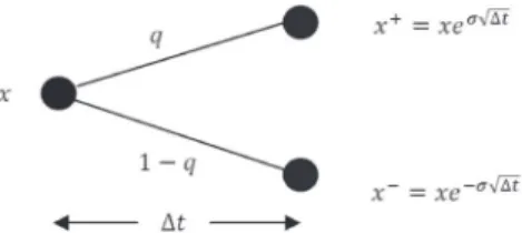
As an illustration, Figure 1 presents the tree for variable X which varies ∆X in the interval
of time ∆t.
Figure 1. Binomial tree for interval of time ∆t
Source: Hahn and Dyer (2011)
The variations of ∆X are as follows:
and . Considering that
represents the natural price logarithm, then
and .
hus:
Eq. 11
Eq. 12
Figure 2. Binomial branch node for prices ()
Source: Hahn and Dyer (2011)
In the assessment of prices, the neutral form of risk to the stochastic process is normally used, so as to be able to discount with the risk-free rate (r). hus, for MRP, the neutral process to risk is given by the following diferential equation
Eq. 13
Where the risk prize is (μ is the total return), and term π/η is a normalized risk prize which penalizes the price logarithm.
Thus, the probability of risk-adjusted Martingale is given by:
Eq. 14
4.2 Bivariate modeling of the Mean
Reversion process
In bivariate modeling, one seeks to combine, in one single tree, two uncertain correlated variables that accompany autoregressive processes. Schwartz and Smith (2000) break down into two factors the natural price logarithm by applying an GBM for the long term and an MRP for the short term. Hahn and Dyer (2011) developed a method for the construction of a bivariate binomial tree that is applicable to the two-factor model of Schwartz and Smith (2000).
Following Hahn and Dyer (2011), the combination of the two variables lead to a quadrinomial tree, as presented in Figure 3.
Figure 3. Bivariate tree (quadrinomial)
Source:Hahn and Dyer (2011)
In the case of the commodities this paper deals with, we presume that the sugar price logarithm (X) and the ethanol price logarithm (Y) follow an MRP. hus,
, and . The relationship
between the increases in the two processes is given by , where ρ is the correlation coeicient.
Hahn and Dyer (2011) use the same basic method used by Boyle (1988) to determine the joint probabilities of the processes. hese probabilities are given by:
Eq. 15
Where the increases are
and . Naturally, the sum of all the
joint probabilities has to be equal to 1, thus
and .The drift of
the processes is given by and
.
out directly, as in the case of one single factor. Given this impossibility, Hahn and Dyer (2011) propose applying Bayesian rules to decompose the joint probabilities in the marginal and conditional
product of the probabilities: .
hus, the marginal probabilities for X would be:
Eq. 16
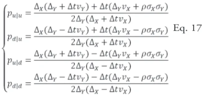
As Equações 15 são divididas pelas probabilidades marginais de X (Equações 16) para se obter as probabilidades condicionais (Equações 17). No presente estudo, as probabilidades apresentadas em Hahn & Dyer (2011) foram corrigidas, pois foram encontrados erros de sinais. A formulação correta, e que foi utilizada neste estudo, é a seguinte:
Eq. 17
Equations 15 are divided by the marginal probabilities of X (Equations 16) to obtain conditional probabilities (Equations 17). In this study, the probabilities presented in Hahn and Dyer (2011) were corrected, since signs of errors were found. he correct formula, which was used in this study, is the following:
The quadrinomial tree with joint probabilities is now divided into two stages of probabilities, conditional and marginal, in the same interval ∆t, for variables X and Y, respectively, which is illustrated in Figure 4. As mentioned, following Nelson and Ramaswamy (1990), in this approach the probabilities are also censored so as not to reach values that are negative or greater than one.
Figure 4. Marginal conditional division of the quadrinomial tree
Source: Hahn and Dyer (2011)
In this new formula the following should
be adhered to: and .
For each of the marginal and conditional probabilities, censorship has to be to the necessary extent.
For the Regions studied in this article (Brazil’s Northeast and Southeast), there are two diferential stochastic equations, one for sugar and one for ethanol:
Eq. 18
Where are the standard Wiener processes in the Northeast for sugar and ethanol respectively, and and , for the Southeast. he processes are correlated
in the following way: , and
.
According to the results of the regressions of the price logarithms of the series used, the values of correlation coeicients that were found are as follows: for the Northeast,
and for the Southeast.
5
Assessment of the switching
option
According to the survey data about the sugar and alcohol production for 2014/15 crops carried out by Brazil’s National Supply Company [Companhia Nacional de Abastecimento, CONAB], Table 4 presents the summary of sugarcane production for the Northeast and Southeast regions, dividing the total by sugar and ethanol products.
Table 4
Production and destination of sugarcane in the Northeast and Southeast regions of Brazil
Sugar and sugarcane industry (1000 Ton.) %Total
Region/states Total Sugar Ethanol Sugar Ethanol
Northeast 55,602 30,963 24,638 55.7% 44.3%
Pernambuco (PE) 14,447 10,107 4,339 70.0% 30.0%
Alagoas (AL) 23,173 16,402 6.771 70.8% 29.2%
Total PE and AL 37,621 26,509 11,111 70.5% 29.5%
Southeast 421,926 214,993 206,933 51.0% 49.0%
São Paulo (SP) 356,283 187,369 168,914 52.6% 47.4%
Source: CONAB - MAPA 2014/2015 crops
In this study, the Northeast region is represented by the states of Pernambuco (PE) and Alagoas (AL), which concentrate 67.66% of the production of sugarcane in this region (37,621/55,602). The Southeast region is represented by the state of São Paulo (SP), which harbors 84.44% of production (356,286/421,926). On the other hand, according to the 2012 CONAB report “Proile of Sugar and Ethanol Industry in Brazil” for Crops 2011/2012 [“Peril do Setor do Açúcar e do Álcool no Brasil” Safra 2011/2012], in the states of Alagoas and Pernambuco operate 46 plants, and in the state of São Paulo there are 169 plants.
With this information, we can determine the quantity (Q) of the annual production of sugarcane by plant in each one of the regions: Northeast (NE) and Southeast (SE).
Regarding productivity rates, Neto and Ramon (2002) mention that, on average, in the state of São Paulo, 93.4 kg of sugar and 76.9 liters of ethanol are obtained per ton of sugarcane. In the Northeast, 92.8 kg of sugar and 65.7 liters of ethanol are obtained per ton of sugarcane.
Considering the sugar and ethanol productivity rates mentioned by Neto and Ramon (2002), and the quantities for each region ( the Gross Revenue (GR) is as follows: GR = Eiciency × Q × Commodity price. hus, one can determine the gross revenue of ethanol and of sugar in a standard plant, for the Northeast and Southeast regions.
Gross Revenue Southeast region:
With the Gross Revenue, one can model the cash low (CF), which can be represented according to Equation 20.
FC= RB[(1-ICMS)-CVT-CFT]×(1-IR) Eq. 20
To determine the components of cash low some considerations were carried out, such as: total variable cost (TVC) is 20% of gross revenue (GR), total ixed cost (TFC) is 10% of
GR, and income tax (IT) is 19% (Bastian-Pinto et al., 2009). hus, the cash lows for the two commodities in the two regions can be modeled in two ways: (1) considering that ethanol is produced exclusively, or (2) considering that the sugar/ ethanol mix provided by CONAB (as shown in Table 4) is produced. In the latter case, it is necessary to consider the proportions of sugar and ethanol to multiply by the production, as follows:
CF in the Southeast Region (in R$1.000): (1) CF considering total production of ethanol:
Eq. 21
(2) CF considering sugar/ethanol production mix:
Eq. 22
CF in the Northeast Region (in R$1.000): (3) CF considering total production of ethanol:
Eq. 23
(4) CF considering sugar/ethanol production mix:
Eq. 24
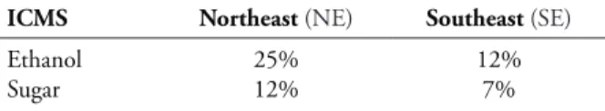
Table 5 presents the ICMS rates for the two commodities in the two regions.
Table 5
ICMS for the Northeast and Southeast regions
ICMS Northeast (NE) Southeast (SE)
Ethanol
Sugar 25%12% 12%7%
Source: CEPEA (2014)
5.1 Assessment using recombinant trees
Capital Asset Pricing Model (CAPM), based on companies in this sector that trade shares on the BMF&BOVESPA (an average of approximately 6% p.a.).
Moreover, using the Equations of Table 2 and the values of the regression coeicients shown in Table 3, the MRP parameters shown in Table 6 are calculated.
Table 6
Parameters of the reversion model for ethanol and sugar in the Northeast and Southeast regions
Parameter Northeast (NE) Southeast (SE)
Ethanol Sugar Ethanol Sugar Initial price (July 2014) 1.5858 57.185 1.3304 47.1785
Long-term average logarithm 0.3970 4.1170 0.2345 4.0036
Long-term average 1.5148 64.9400 1.3088 59.1207
Volatility (σ) 0.2561 0.2999 0.3879 0.3330
Reversion speed (η) 1.7901 0.7979 2.1723 0.7306
With the calculated parameters, and following the procedure described in section 4.1, one can calculate the binomial tree. Using the censored approach of Nelson and Ramaswamy (1990), the probabilities are calculated by
To save space in the text, we will not present the illustration of binomial trees generated for the prices and probabilities. hey are available from the authors at request.
Based on the simulated prices of sugar and ethanol, sugar cash lows in the Northeast region are calculated using equation 24 over a 5-year period (T= 5). Using the risk-free rate and the censored Martingale probabilities, through the backward (Cox et al., 1979) process, the value of the cash low is determined for point t = 0.
Present value, PV, (at point t = 0) of the cash lows for sugar in the Northeast region (NE) is R$ 394.79 thousand. A similar procedure was used for ethanol in the NE region, and sugar and ethanol in the SE region. In this way, Table 7 shows the present values (PV) for the four approached situations.
We observe that the PV is greater for the Southeat region, for both commodities. For the
case of ethanol, the diference between the two regions represents a 242% diference favorable to the Southeast region. For the case of sugar, on the other hand, the PV diference represents an 177% percentage.
Table 7
Present values (PV) of the cash lows of the recombinant trees (in R$ 1.000)
Region Ethanol Sugar
Northeast (NE)
Southeast (SE) 272.28930.42 1.093.25394.79 Diference 658.14 698.46 Diference (%) 241.7% 176.9%
5.2 Assessment using bivariate trees
marginal and conditional probabilities, which, when multiplied, result in the joint probabilities.
Table 8 presents, for the two regions studied, the results of the present values (PV) of
cash lows for plants that produce ethanol or sugar (sugar/ethanol mix), and the present value (PV) of cash lows for lexible plants.
Table 8
Results of the present values (PV) of the cash lows, of the binomial and bivariate trees and the value of the Switching Option (in R$1.000)
Binomial Tree Quadrinomial Tree Value of the Switching Option
PV Ethanol Plant
PV Sugar Plant
Flex Plant
% Dif. Ethanol Plant
% Dif. Sugar Plant
From Ethanol to Flex
From Sugar to Flex
(1) Northeast 272.28 394.79 432.71 58.9% 9.6% 160.43 37.92
(2) Southeast 930.42 1.093.25 1.616.11 73.7% 47.8% 685.69 522.86
Diference (2-1) 658.14 698.46 1.183.40 525.25 484.94
% Diference 241.% 175.9% 273.5% 327.4% 1278.8%
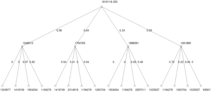
Figure 5. Present value (PV) of the cash lows for the bivariate quadrinomial tree of the Northeast region
he results shown prove that, in the case of the Northeast, the lex plant has a higher value (higher PV) when compared to a plant that produces sugar (sugar/ethanol mix); the diference is 9.6%. As for the comparative case of a plant whose production is focused exclusively
Figure 6. Present value (PV) of the cash lows for the bivariate quadrinomial tree of the Southeast region
In the case of the Southeast, the diference in favor of flex is 73.7% and 47.8%, when compared to a plant that produces only ethanol and one that produces sugar (sugar/ethanol mix), respectively. his means that the decision to use the lex plant increases the present value of the business in R$ 686 million when compared to ethanol production, and R$ 522 million, when compared to sugar production.
hese gains, both in the Northeast and in the Southeast, occur despite the greater eiciency in sugar production compared to ethanol (note the eiciency parameters in the equations that compute the Gross Revenue). his means that the investment in lexibility for the construction of a lex plant is advantageous to the levels of the mentioned gains. That is, the additional investment in the lex plant compared to a non-lex plant should not be smaller than the gain derived from the operation of changing the production of one product to another throughout the plant’s productive life.
After identifying the gains from operating lexible plants, two aspects should be highlighted. The first one refers to the investing agent: investing in inlexible systems means neglecting this gain (i.e. “leaving money on the table”). he second one refers to the regulating agent: a lexible plant results in greater gains for the
investor and, therefore, more tax collection (ceteris paribus), and this means that there is room for tax policies aimed at encouraging the construction of lexible systems. In short, the possibility of increasing lexibilization depends on the investor’s knowledge of potential gains and incentives for the construction of such systems by regulating authorities.
In the case of the value of the lexibility (switching) option, we observed that this value in the Southeast region is more signiicant when compared to the Northeast. This was to be expected, because the comparative advantages (smaller ICMS and greater production) are better in this region. For both regions, Table 8 shows that lexibility adds a signiicant value. We observed that, in the case of ethanol, the switching option value is 327.4% greater in the Southeast than in the Northeast. he same applies to the case of sugar, where, for the Southeast, this option’s value is 1278% greater than in the Northeast.
6
Conclusions
clean production mechanisms. he potential for production and the increase in demand for ethanol make sugarcane one of the most important crops in the current Brazilian agribusiness scenario. Sugarcane is not just another national agricultural product, but the most important source of biomass energy, because of the potential of the sugar and ethanol industry in Brazil.
According to the aspects described and the results generated in the development of this article, we can conclude mainly that the value of the switching option in the sugar and alcohol sector is associated with determining factors. First, the production of sugarcane by region, highlighting the Southeast region which, according to the 2014/15 crops, produces 421,926,000 tons of sugarcane, against 55.602 million tons in the Northeast (sugarcane production from the Northeast region adds up to 38% of the Southeast region production). Another important factor is ethanol’s eiciency ratio in the Southeast, which is 76.9 L/ton, while in the Northeast it is only 65.7 L/ton. On the other hand, the ICMS tax afects the sugar and alcohol industry revenue in a signiicant way; the Southeast has greater tax incentives (ICMS 12% for ethanol and 7% for sugar), while in the Northeast the rates are higher (25% ICMS for ethanol and 12% for sugar).
By modeling commodity prices through MRP and using quadrinomial trees with censored probabilities, we determined the value of the switching option embedded in plants with lexible production (lex plants); according to the values that were found, we conclude that factors such as the level of production and the tax burden, combined with commodity prices, affect the value of the switching option in a relevant way, and that lex plants are always more advantageous than plants that only produce ethanol or sugar. In the study results we found that the plants in the Southeast have a higher cash low present value than the plants located in the Northeast, mainly due to their higher production level and to the considerably lower taxation they face. hus, these components must not be disregarded
when performing the analysis of the value of the lexibility option for lex-type plants in the Brazilian sugar and alcohol sector.
One of the contributions of the study, as proven by the results, are the implications for policies focused on this sector. he results show that it is more attractive for producers to invest in lexible plants. hus, they can take advantage of ethanol production and of sugar production, according to the convenience of product prices. hus, a lexible plant will remain in operation for a longer period of time, and always operate in an optimal situation in terms of revenue. Consequently, it will contribute more taxes both on state and federal level. herefore, the regulators will have more space to prepare tax incentive policies for the construction of lexible systems. his is important, especially for the Northeast region, where the tax burden is high when compared to the Southeast.
Note
1 he authors would like to thank the two anonymous
reviewers for their suggestions, which helped improve the quality of this study. The remaining errors or omissions are our responsibility.
References
Aiube, F. A. L., & Samanez, C. P. (2014). On the comparison of Schwartz and Smith’s two-and three-factor models on commodity prices. Applied Economics, 46(30), 3736-3749.
Balcombe, K.; Rapsomanikis, G. (2008) Bayesian Estimation and selection of nonlinear vector correction models: the case of the sugar-ethanol-oil nexus in Brazil. American Journal of Agricultural Economics. 90(3) August: 658–668
Bastian-Pinto, C., Brandao, L., & Hahn, W. J. (2009). Flexibility as a source of value in the production of alternative fuels: he ethanol case. Energy Economics, 31(3), 411-422. doi: DOI 10.1016/j.eneco.2009.02.004
Bessembinder, H., Cougehnour, J., Seguin, P., & Smoller, M. (1995). Mean reversion in equilibrium asset prices: Evidence from futures term structure. Journal of Finance, vol 50(1), 361-375.
Black, F., & Scholes, M. (1973). he Pricing of Options and Corporate Liabilities. he Journal of Political Economy, 81(3), 637-654.
Bof H. P. (2011) Modeling the Brazilian Ethanol Market: How Flex-Fuel Vehicles are Shaping the Long Run Equilibrium, China-USA Business Review,10 (4), 245-264.
Boyle, P. A. (1988). A Lattice Framework for Option Pricing with Two State Variables. Journal of Financial and Quantitative Analysis, 23(1), 1-12.
Cavalcante, H. P. M. (2010). Aspectos relativos ao etanol brasileiro e as barreiras não-tarifárias à sua importação, jurídicos Direto E-nergia, Ano II, vol 2, January-July. Available at: <http://periodicos. ufrn.br/direitoenergia/article/viewFile/4238/3474>
CEPEA. Available at: <http://www.cepea.esalq.usp. br>. Access on: 02 de maio de 2014.
COSENCANA-SP. Available at: <http://www. consecana.com.br/>. Access on: 20 de maio de 2106.
Cox, J. C., Ross, S. A., & Rubinstein, M. (1979). Option pricing: A simpliied approach. Journal of Financial Economics, 7(3), 229-263. doi: Doi: 10.1016/0304-405x(79)90015-1
Dixit, A. K., & Pindyck, R. S. (1994). Investment under Uncertainty. Princeton: Princeton University Press.
FGV-IBRE. Available at: <http://portalibre.fgv.br>. Access on: 09 de maio de 2014.
Hahn, W. J. (2005). A Discrete-Time Approach for Valuing Real Options with Underlying Mean-Reverting Stochastic Processes. (PhD Dissertation), he University of Texas, Austin.
Hahn, W. J., & Dyer, J. S. (2011). A Discrete Time Approach for Modeling Two-Factor Mean-Reverting Stochastic Processes. Decision Analysis, 8(3), 220-232. doi: 10.1287/deca.1110.0209
Lima, N. C., De Oliveira, S. V. W. B., De Oliveira, M. M. B., & Queiroz, J. V. (2013). Caracterização da demanda do combustível etanol hidratado no mercado brasileiro. Gestão Contemporânea (13), 25-44.
Macedo, I. C. (2007). Situação atual e perspectivas do etanol, Estudos Avançados, 21(59). Available at: http://www.scielo.br/pdf/ea/v21n59/a11v2159.pdf
Melo, A. S.; Sampaio, Y. (2016) Uma Nota Sobre o Impacto do Preço do Açúcar, do Etanol e da Gasolina na Produção do Setor Sucroalcooleiro. Revista Brasileira de Economia. v. 70 n. 1 / p. 61-69.
Moraes, M. A. F. D (1999). A desregulamentação do setor sucroalcooleiro brasileiro. Tese de doutorado, Departamento de Economia, Universidade de São Paulo.
Nascimento, C. C (2012). O valor da opção do carro Flex por região geográica do Brasil: uma aplicação da Teoria das Opções Reais com Movimento de Reversão à Média. Rio de Janeiro, RJ, Masters’ Dissertation. PUC-Rio.
Nelson, D. B., & Ramaswamy, K. (1990). Simple Binomial Processes as Difusion Approximations in Financial Models. Review of Financial Studies, 3(3), 393-430.
Neto, V. C., & Ramon, D. (2002). Análises de opções tecnológicas para projetos de co-geração no setor sucro-alcooleiro. Brasília, DF.
Samanez, C. P., & Costa, L. d. A. (2014). Avaliação de opções de swing em contratos de gás natural usando um modelo de dois fatores. Production Journal, 24(4), 760-775.
Samanez, C. P., Ferreira, L. d. R., & Do Nascimento, C. C. (2014). Avaliação da opção de troca de combustível no carro brasileiro lex: um estudo por região geográica usando teoria de opções reais e simulação estocástica. Production, 24(3), 628-643.
Schwartz, E. S. (1997). he stochastic behavior of commodity prices: Implications for valuation and hedging. he Journal of Finance, 3(52), 923-973.
Schwartz, E., & Smith, J. E. (2000). Short-Term Variations and Long-Short-Term Dynamics in Commodity Prices. Management Science, 46(7), 893-911. doi: 10.1287/mnsc.46.7.893.12034
Tourinho, O. A. F. (1979). he valuation of reserves of natural resources: An option pricing approach. PhD thesis, University of California, Berkeley, 1979.
Trigeorgis, L. (1996). Real Options: Managerial lexibility and strategy in resource allocation, MIT Press.
About the authors:
1. David Eduardo Lopez Pantoja, MSc. in Production Engineering, PUC-RJ, Brazil. E-mail: [email protected].
2. Carlos Patricio Mercado Samanez (in memoriam), PhD in Management, Getúlio Vargas
Foundation-SP, Brazil.
3. Javier Gutierrez Castro, PhD in Production Engineering, UTFPR, Brazil. E-mail: [email protected].
4. Fernando Antonio Lucena Aiube, PhD in Production Engineering, PUC-RJ, Brazil. E-mail: [email protected].
Contribution of each author:
Contribution David Eduardo Lopez Pantoja Mercado SamanezCarlos Patrício Javier Gutierrez Castro Fernando Antonio Lucena Aiube
1. Deinition of research problem √ √
2. Development of hypotheses or research
questions (empirical studies ) √ √
3. Development of theoretical propositions
(theoretical Work ) √ √
4. heoretical foundation/Literature review √ √ √ √
5. Deinition of methodological procedures √ √
6. Data collection √
7. Statistical analysis √ √ √ √
8. Analysis and interpretation of data √ √ √ √
9. Critical revision of the manuscript √ √ √ √
10. Manuscript Writing √ √ √ √