A Multi-Objective Unit Commitment Model for Setting Carbon Tax to Reduce CO2 Emission: Thailand's Electricity Generation Case

A Multi-Objective Unit Commitment Model for Setting Carbon Tax to

Reduce CO2 Emission: Thailand’s Electricity Generation Case

Nuchjarin Intalar, Apirath Phusittrakool, Chawalit Jeenanunta, Aussadavut Dumrongsiri and Pisal Yenradee Sirindhorn International Institute of Technology, Thammasat University,

P.O. Box 22, Thammasat Rangsit Post Ofice, Pathumthani 12120, Thailand

Abstract

Carbon tax policy is a cost-effective instrument for emission reduction. However, setting the carbon tax is one of the challenging task for policy makers as it will lead to higher price of emission-intensive sources especially the utility price.

In a large-scale power generation system, minimizing the operational cost and the environmental impact are conlicting objectives and it is dificult to ind the compromise solution. This paper proposes a methodology of inding a feasible carbon

tax rate on strategic level using the operational unit commitment model. We present a multi-objective mixed integer linear

programming model to solve the unit commitment problem and consider the environmental impacts. The methodology

of analyzing of the effect of carbon tax rates on the power generation, operating cost, and CO2 emission is also provided.

The trade-off relationship between total operating cost and total CO2 emission is presented in the Pareto-optimal curve to

analyze the feasible carbon tax rate that is inluencing on electricity operating cost. The signiicant outcome of this paper

is a modeling framework for the policy makers to determine the possible carbon tax that can be imposed on the electricity generation.

Keywords: CO2 emission reduction; multi-objective unit commitment; carbon tax policy; pareto-optimal curve; energy policy

1. Introduction

Global warming and carbon dioxide (CO2) emissions reduction have become important issues. The power sector is a major CO2 polluter in many countries. Under the pressure of global warming, it is crucial for government to impose the effective policy to promote CO2 emission reduction. Thailand’s CO2 emissions levels are continuing to rise in accordance with the increased volume of national energy consumption.

There are several policies introduced to reduce CO2 emissions. The most widely proposed is a carbon tax policy because it is a cost-effective instrument for emission reduction (Baranzini et al., 2000; Nagurney et al., 2006). Carbon tax is the tax paid by polluters who emit CO2 from burning fossil fuels and releasing CO2 into the atmosphere. In fact, CO2 emissions are already implicitly taxed in every country even in those developing countries that the Kyoto protocol has not targeted (Baranzini et al., 2000). However, setting the carbon tax is a challenging task for policy makers as it will lead to higher price of emission-intensive sources, especially utility prices. The different carbon tax rate imposed in each country depends on the regulation and several factors.

Several researchers have formulated mathematical models and applied tools such as the HERMES

macroeconomic model (Cosmo and Hyland, 2013) and the dynamic Computable General Equilibrium (CGE) model (Wachirarangsrikul et al., 2013; Thepkhun et al., 2013) to explore the impact of the taxation of CO2 on national economies that undertake carbon reduction in the future. Some of the studies estimate the optimal or appropriate carbon tax to impose on the electricity cost (Lu et al., 2010). Most of the studies divided the carbon tax into three scenarios which are a baseline (carbon tax is zero), the average carbon tax rate, and high tax rate. The results show that the CO2 emission can be signiicantly reduced by imposing the fairly moderate tax rate (Wachirarangsrikul et al., 2013) and highest carbon tax (Cosmo and Hyland, 2013). The carbon tax policy shows the effectiveness and potential of CO2 emission reduction and the positive impact on the economic and environmental improvement in long term. Although, the proposed carbon tax rate shows the signiicant reduction of CO2 emission, it cannot suggest a policy maker how much it costs to reduce the CO2 emission to a certain amount based on the current carbon tax rate in Thailand and existing power generation capacity. It is important for the strategic policy maker to work in a cost effective way to reduce CO2 emissions while maintaining minimum operating cost. In spite of this, the power sector intends to improve the operating eficiency and reduce overall operation

The international journal published by the Thai Society of Higher Education Institutes on Environment

E

nvironment

A

sia

Available online at www.tshe.org/EA EnvironmentAsia 8(2) (2015) 9-17

10 costs as much as possible while satisfying all demands.

Power generation planning is a challenging task because of the complications of the generation process, transmission, and generation of electric power which lead to a variety of issues in decision making. The power generator uses the unit commitment (UC) model to plan the operation of the generator unit whether to turn the unit on or off and the amount of power to be generated in each period. In general, the UC model is used to minimize the operating cost which mainly include the fuel cost. In this paper, the multi-objective unit commitment model is proposed with two conlicting objective functions: minimization of the operating cost and CO2 emission. In the multi-objective problem, an optimal solution is generally more dificult to ind. Therefore, the compromise solution can be the best for all conlicting objectives. Many solutions are presented in the Pareto-optimal solutions on a trade-off curve between the fuels cost and emission costs by using a multi-objective optimization (MO) model (Catalão et al., 2008) and another using the decommitment procedure of unit commitment (Yamashita et al., 2010). These solutions showed the trade-off points on the curve for a decision maker to select. However, the studies did not take a carbon tax into account. The models are tested on the simulated model which contains only 10 generating units (Yamashita et al., 2010).

From the strategic policy level view point, the impacts of various carbon tax rates on the operational level of unit scheduling are investigated. By considering different rates of the carbon tax, the impacts of CO2 emission from strategic level planning that lead to the effect on the unit schedules and power generations of power system at the operational level are investigated. The model is coded and solved by using a commercial

optimization package, IBM ILOG CPLEX, which is a computationally eficient solver that can handle large scale mixed integer programming problems.

2. Materials and Methods

2.1. Data of case study

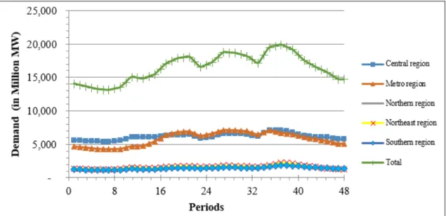
A case study of a large scale power generation system in Thailand is used to demonstrate the methodology. The system comprises the combination of the thermal, gas turbine, hydro and combined cycle generators which are 51 power plants and 171 generators. The power plants are located in ive main regions of Thailand: central, metro, north, northeast, and south regions. There are ive main sources of fuel types: natural gas, coal/lignite, hydro, fuel oil, and diesel oil. The generating units generate electricity by using different types of fuel. Each fuel type has a different eficiency, price and CO2 emission intensity. For daily planning, input of the models is the demand on Monday 12 October, 2011 which directly obtained from EGAT. The time period is started from 12:00 AM of day one until 12:00 AM of day two. It is scheduled in a half-hour schedule with a time horizon of 24 hours (48 periods) with the time slot of 30 minutes as shown in Fig. 1.

There are two fuel modes in each generator which are the single and mixed fuel mode. The single fuel mode means the generating unit is allowed to use only one type of fuel to generate electricity. The mixed fuel mode means the generating unit is allowed to mix two types of fuel and the mixture is considered as a new fuel type.

The combination of fuel types produces different levels of CO2 intensity. Therefore, we assign different

11 values of CO2 intensity depending on the fuel type usage of each generating unit. The CO2 intensity for each generator and fuel is shown in Table 1. For carbon tax imposed in Thailand, in order to estimate a carbon tax in Thailand, a baseline for setting a carbon tax is “Social cost of carbon (SCC)”. The social cost of carbon (SCC) is used by United States Environmental Protection Agency and other federal agencies to estimate the economic damages associated with a small increase in CO₂ emissions. However, the exact value of SCC is not deined. There are more than 200 estimated values of SCC starting from 15 baht/tCO2 to 24,000 baht/tCO2 (Policy Brief). Since, Thailand has not practically been imposed a carbon tax on electricity cost, therefore, this paper relies a carbon tax rate on IPCC Emission Trading value in 2009. Based on the Intergovernmental Panel on Climate Change (IPCC), an average carbon tax for Emission Trading Scheme (ET) in Europe Emission Trading Scheme (EU ETS) in 2009 is 349 baht/tCO2 (Wattanakulcharat and Wongsa, 2011).

2.2. Problem Formulation

In this section, two models are introduced and formulated; the operating cost minimization (Model A) and the utility optimization model (Model B).

2.2.1. Operating Cost Minimization Model (Model A)

The model is formulated to solve the unit commitment (UC) problem to minimize total operating cost regardless of the CO2 emission. The proportion of the fuel usage for each type is obtained by this model.

1) Objective Function: The objective function is the minimization of the total operating cost which includes the fuel cost and the startup cost of the generating units over the planning horizon, subjected to the load demand and other individual unit constraints such as the fuel usage. The objective function is formulated as follows:

(1)

Where I is set of power generating units (thermal, gas turbine, combined cycle and hydro), T is the length of the planning horizon, U is the total number of the generating units, F is the set of fuel types (lignite, natural gas and diesel oil).

The fuel cost function is calculated by the multiplication of cost of fuel type f used in unit i (cif),

the amount of fuel used in unit i at time t (FUt), and the production of unit i at time t (Pt).

The startup cost (SCi) is the cost charged when

any generating unit is started to generate the electricity. If the unit i is started at time t, st has value of 1 and 0 otherwise. The startup cost is calculated by the startup cost of unit i multiplied by startup status.

2) General System and Unit Constraints:

System Load Balance Constraint: There are ive zones of power generation in Thailand which are central, metro, northern, northeast, and southern zones. The total amount of production of unit i in zone z at time t (Pt) plus the total of power transmitted through transmission line from demand zone i to demand zone

j at time t (Lt) minus the amount of water pumped by pump k in plant p at time t (pwt ) must meet load demand d in zone z at time t (dt). We also consider the transmis-sion line capacity among zones and the pump power in this equation. The constraint is expressed as follows:

(2)

General Unit Constraints: This constraint is the turn on/off status for each generating unit. If the unit i is already operating when this scheduling horizon starts, then it is not turned on at the start as (3). If the unit i is already on when this scheduling horizon starts, then it will either be turned off at time 1 or remain operating at time 1 as (4). If the unit i is off when this scheduling horizon starts, then it is not turned off at the start as (5). If the unit i is off when this scheduling horizon starts, then the turn on variable must be the same as operating variable as (6). If the unit i is off at time t and on at

Table 1. CO2 emission intensity value

Generator Type Fuel Type kgCO2/MWha

Thermal

The combination of natural gas, fuel oil, and diesel oil 622

The combination of natural gas and fuel oil 600

Lignite 914

Gas Turbine The combination of natural gas and diesel oil 469

Combined Cycle The combination of natural gas and diesel oil 469

Natural gas 426

Sources:a _{adopted from Sutham (2011) and EGAT (2010)} usage. The objective function is formulated as follows:





   

    

 

  

 

   

 

 

I i t T

t i i U

u f F

t i t i i

f FU P SC s

c Min

Where I is set of power generating units (thermal, gas turbine,

















 





   

    

   

  

 

   

 

 

T

t

Z

z

d

pw

L

p

zt

t kp k j t ij j z i t iz I i

















 

,

,

=

,

=

i

i

i

iz

z ij

12 time t+1, then it was turned on at time t+1 as (7). The constraints are expressed as follows:

(3) (4) (5) (6) (7)

Generation Limit Constraint: The power generation from the generating unit i at time t has upper and lower bound limits. The constraint is expressed as follows:

(8)

Ramp-Up/Down Constraints: The generating unit’s ramp-up (φ) and ramp-down (φ) rate at time t. For each ramping, we divided the equation into two stages which are the initial stage and the processing stage. Constraint (9) and (10) are the initial stages for up and ramp-down, respectively. Constraint (11) and (12) are the ramp-up and ramp-down limitation, respectively. The constraints are expressed as follows:

(9)

(10) (11) (12)

Minimum Up/Down Time Constraints: When the unit i is scheduled to start-up or shutdown, it has a duration of minimum up time (εi) or minimum down

time (εi) before the unit is startup or shutdown because

the generating unit cannot be immediately turned on or turned off. The constraints of minimum up/down time are expressed in (13) and (14) as follows:

(13)

(14)

Fuel Usage Constraints: There are two constraints for the fuel usage limitation. First, the total amount of fuel usages f of the unit i in plant p at time t (qt ) must not exceed the maximum amount of fuel f available

for plant p (qmax). Second, the generating unit i cannot use more than one type of fuel f at time t (FUt). The constraints are expressed as follows:

(15) (16)

Spinning Reserve Constraint: The spinning reserve is provided to compensate when shortfalls occur. The total spinning reserve is greater than or equal to the spinning reserve required ( ). The constraint is expressed as follows:

(17)

2.2.2. Utility Optimization Model (Model B)

The utility optimization model (Model B) is formulated using the multi-objective unit commitment technique to find the compromise solution that minimizes both operating cost and CO2 emission cost. The CO2 emission is converted to monetary cost by using the carbon tax rate. The objective consists of the fuel costs, start-up cost, operating cost, and CO2 emission costs. The formulation are presented as follows.

1) Objective Function: The objective function is the minimization of the total cost as formulated below:

(18)

(19)

The CO2 emission cost is the CO2 emission intensity from generating unit i (Ei) multiplied by the

total production (Pt) and carbon tax rate from generating unit i (CTi). The CO2 emission intensity (Ei) is calculated

by fuel consumption (FCi) multiplied by Emission Factor for each fuel type (Ef). The default value of

emission factor is obtained from Revised 2006 IPCC Guideline for National Greenhouse Gas Inventories. Model B contains objective function with constraints (2)-(17).

3. Results and discussion

In this section, the analysis of the results obtained

1 0

= 0

{

|

> 0}

i S i

s

  

i

I

I

p

0}

|

{

1

0

1

1













i S i

i

o

i

I

I

p

s

0}

|

{

0

0

1











i S i

i

I

I

p

s

1 1 0

=

{

|

= 0}

i i S i

s

o

  

i

I

I

p

1 1

,

{1,

,

1}

t t t

i i i S

o



 

o

s



  

i

I

I

t





T







































~













_

_











_

~

_

















 

















 

  























  



_{ }



_{  }

_

_



p

o

p

p

o

_it _imin



_it



_it _imax

































~













_

_











_

~

_

















 

















 

  























  



_{ }



_{  }

_

_



T

t

I

i











,



























~













_

_











_

~

_

















 

















  %

  























  



_{ }



_{  }

_

_

_















I

i

p

p

_i1



_i0





_i







I

i

p

p

_i0



_i1





~

_i







I

i

p

p

_it1



_it





_i







I

i

p

p

i t i t

i









1

_

~

_

















 

















  %

  























  



_{ }



_{  }

_

_

_

















































_

_











_

_



inimum up/down time are expressed in (1

}

>

|

{

,

t

T

t

_i

I

i















 

}

~

>

|

{

,

t

T

t

i

I

i

















 

  























  



_{ }



_{  }

_

_

_

















































_

_











_

_



turned off. The constraints of minim

1 = ' t i t i t i t t

o

s















 

1

~

1 ~ = ' t i t i t i t t

o

s

















  ip ip i i i max fp t fip I i T t

F

f

P

p

q

q













 

,

I

i

FU

_it

F f











1

Spinning Reserve Constraint: The spinning reserve is provided to com



















 



   

                      















 













T

t

p

o

p

_imax _it _it

I i















)

(



 



   

                      















 

























 formulated below:



 



   

                       I

i t T u U f F

t i t i i

f FU P

c Min















 





























 



   

                       i t i i t i i t CT P E s SC P FC















 





























 



   

                      

CO2 emission for each generation: Ei = i f

FC



Ef

The CO emission cost is the CO emission intensity

i

13 from the Operating Cost Minimization Model (Model A) and the utility optimization model (Model B) is presented. These models were formulated to ind the compromise solution that satisies both strategic and operational levels.

3.1. Compromise Solution of Operating Cost, CO2

emission Cost and CO2 emission

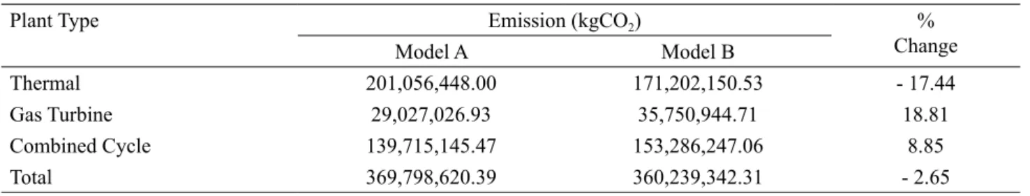
In this section, we present the result of Model A and B using the mixed integer programming. The comparison is divided into three terms which are the total operating cost, the total CO2 emission cost and the total CO2 emission. For the total operating cost comparison, the Utility Optimization Model (Model B) has only 0.28 percent higher cost than the Operating Cost Minimization Model (Model A) which is considered acceptable. For the total CO2 emission cost, Model B is 1.23 percent lower than Model A. Moreover, the total CO2 emission from Model B is lower than Model A approximately 4.82 million kilograms of carbon dioxide (kgCO2) or 4,816 tons of carbon dioxide (tCO2). Once, the multi-objective unit commitment approach is applied, Model B is not only minimize total operating cost, but also the total CO2 cost. Therefore, the main generators are in combined cycle power plants which lead to a lower amount of coal-ired consumption. Therefore, the CO2 emission is signiicantly dropped.

The results of CO2 emission comparison are shown in Table 3. The unit commitment optimization approach decreases the overall emission by 2.65 percent from Model A. The total proportion of emission of Model B from the thermal plants is decreased by 17.44 percent. The emission from the gas turbine and combined cycle plants are increased by 18.81 and 8.85, respectively. The system reduces the usage of lignite and shift to natural

gas instead. The natural gas is typically expensive; therefore, it leads to higher total cost in Model B than Model A. Once the CO2 emission cost is involved in the objective function, the proportion of fuel type consumption is changed. For Model B, the fuel usage of lignite in thermal generator is decreased by 20.15 percent and the usage of natural gas is increased by 21.05 percent.

3.2. Sensitivity Analysis

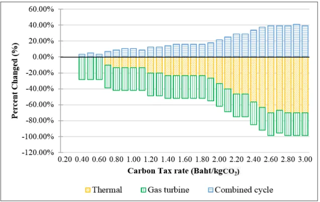
In this section, the sensitivity analysis of Model B shows the comparison of the power generation for each generator by varying the carbon tax rates from 0.10 - 3.00 baht/kgCO2 (Fig. 2). The high carbon tax rate directly impacts the behavior of power generation, especially for the thermal and combined cycle plants.

There is no signiicant change when the carbon tax rate is between 0.10 and 0.60 baht/kgCO2 which indicates that the prices are too small to trigger the change of system behavior compared with the operating cost. However, change occurs slowly when the prices are between 0.70 and 1.80 baht/kgCO2. The proportion of combined cycle plant is slowly increased while the thermal plant is slowly decreased. The obvious change is occurred when the price is greater than 1.90 baht/ kgCO2.

The stacked chart of percent changed of power generation for thermal, gas turbine, and combined cycle plant is shown in Fig. 3. At the rate of 0.70 baht/ kgCO2, the generation from thermal starts to decrease by 10 percent while the combined cycle is increased by 7.14 percent. This shows the carbon tax has higher effect than the operating cost in the thermal plant. On average, from the rate of 0.20 - 1.90 baht/kgCO2, the generation from thermal is decreased by 14.74 percent while the combined cycle is increased by 10.02 percent.

Table 2. Total cost comparison for each model

Model CO2 Emission Cost (THB) Total Operating Cost (THB) Operating Cost Minimization Model 136,723,966.31 633,856,023.21

Utility Optimization Model 135,043,207.04 635,609,670.08

Table 3. Emission comparison for each power plant type

Plant Type Emission (kgCO2) %

Change

Model A Model B

Thermal 201,056,448.00 171,202,150.53 - 17.44

Gas Turbine 29,027,026.93 35,750,944.71 18.81

Combined Cycle 139,715,145.47 153,286,247.06 8.85

14 The signiicant change obvious occurs when the price is greater than 2.00 baht/kgCO2. On average, from the rate of 2.00 - 3.00 baht/kgCO2, the generation from thermal is decreased by 57.58 percent while the combined cycle is increased by 33.93 percent. This leads to higher CO₂ emission reduction.

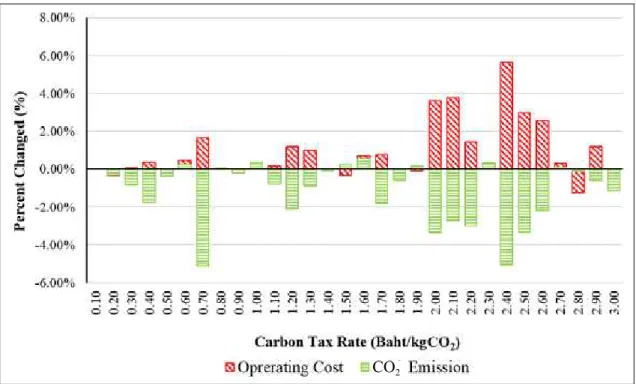
Fig. 4 shows the percentage of change of the operating cost and the CO2 emission when the carbon tax rate is increased by 0.10 baht/kgCO2. There are

called the marginal operating cost and the marginal CO2 emission, respectively. The obvious trade-off between the operating cost and the CO2 emission occurs at the price of 0.70 baht/kgCO2. The CO2 emission is decreased by 5.13 percent while the operating cost is increased only 1.66 percent. For the based case, the imposition of carbon tax at 0.349 baht/ kgCO2 reduces approximately 1.96 percent while the total operating cost increases by only 0.04 percent. Figure 2. Sensitivity analysis of the power generation for each plant type to the carbon tax

15

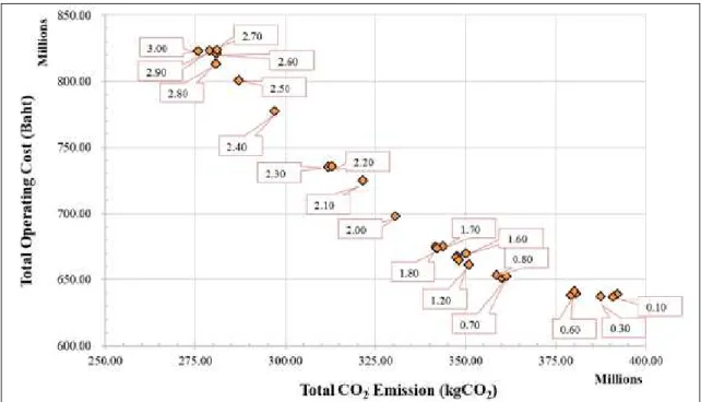
3.3. Pareto-Optimal Analysis of Utility Optimization Model

In this section we present the Pareto-Optimal analysis by using the eficient frontier graph between the total operating cost and the CO2 emission of the utility optimization model. It is illustrated as a guideline for a strategic planner to determine the compromise solution for the power generation based on environmental considerations. Besides, we suggest the methodology to set an appropriate carbon tax that maximizes the reduction of the CO2 emission while the operating cost increases in the lowest proportion.

The trade-off graph of Model B is obtained by plotting the point representing the total operating cost and total CO2 emission for each carbon tax rate as shown in Fig. 5. This graph shows the different behavior of the increment of the total operating cost over the decrement of the total CO2 emission as the carbon tax rate increased. The marginal CO2 emission is the change in the CO2 emission when the carbon tax has an increment by unit. The marginal operating cost is the change in the operating cost when the carbon tax has an increment by unit.

When the carbon tax is changed from 0.60 to 0.70 baht/kgCO2, the marginal CO2 emission is decreased by 6.30 percent while the operating cost is increased only 1.72 percent. The rate of change of the operating cost and the CO2 emission is 1:4. From 1.90 to 2.00 baht/kgCO2, the marginal reduction of CO2 emission is equal to the marginal increment of operating cost

which is 3 percent. From 2.40 to 2.50 baht/kgCO2 and the marginal reduction of CO2 emission is equal to the marginal increment of operating cost which is 5 percent. The suggestion from this relationship is the approapriate carbon tax range that can decreased large proportion of CO2 emission is between 0.60 to 0.70 baht/kgCO2. In the utility optimization model, the carbon tax at any rate can be set to test the effect of the operating cost and the CO2 emission instantly. Therefore, the computational time of the utility optimization model is fast and continent.

4. Conclusions

This paper presented a modeling framework to determine the possible carbon tax rates that can be imposed on the electricity operating cost for the policy makers. It was signiicant to know the best achievable level of the total operating cost and the CO2 emission based on the capacity of existing power generators. The Utility Optimization model was proposed in this paper to generate a good compromise solution for a multi-objective unit commitment problem in large-scale power generation planning. The operating cost was increase in small proportion compared with large amount of CO2 emission it reduced. The trade-off relationship between the operating cost and CO2 emission and the marginal cost of CO2 reduction were illustrated to use as a guideline for a planner to make an optimal decision for the unit commitment dispatch with the acceptable emission allowance.

Figure 4. The increase in percent of total operating cost and reduction of the emission

16 The possible carbon tax rate that can be imposed to reduce CO2 emissions in long term is between 0.60 to 0.70 baht/kgCO2. In order to set the carbon tax on electricity cost, it is needed the involvement of government ofice and related parties. The appropriate carbon tax rate setting will lead to CO2 emissions reduction in a long term. In the beginning phase, the lower carbon tax rate can be imposed on electricity cost to observe the impact on different perspective by using the carbon tax rate of 0.349 baht/kgCO2 as a baseline. It might be applied for a few years. Once the CO2 emissions can be decreased by this policy, the government sector can increase the carbon tax rate and reduce more emissions. The options that can be used to limit the CO2 emissions from electricity generation include increasing the usage of renewable energy, using fuels with lower CO2 emission per kWh produced and/or increasing the efficiency of the electricity production. In future research, the model should consider the share of renewable energy and formulate the equation that also involved renewable energy. Acknowledgments

The authors gratefully acknowledge the support of Grant 51-2115-023-JOB NO.544-SIIT from EGAT and

the BCP Research Grant from Bangchak Petroleum Public Company Limited (BCP).

References

Baranzini A, Goldemberg J, Speck S. A future for carbon

taxes. Ecological Economics 2000; 32(3): 395-412.

Catalão JPS, Mariano SJPS, Mendes VMF, Ferreira LAFM.

Short-term scheduling of thermal units: emission constraints and trade-off curves. European Transactions on Electrical Power 2008; 18(1): 1-14.

Cosmo VD, Hyland M. Carbon tax scenarios and their effects

on the Irish energy sector. Energy Policy 2013; 59:

14.

Energy Policy and Planning Ofice Ministry of Energy. Energy Statistics of Thailand 2012. Report.

Electricity Generating Authority of Thailand (EGAT). Power Development Plan 2010 (PDP2010). EGAT, Bangkok, Thailand. 2010.

IPCC Guidelines for National Greenhouse Gas Inventories.

Chapter 2, Equation 2.1, Energy; 2: 2.11. 2006.

IPCC Guidelines for National Greenhouse Gas Inventories.

Chapter 2, Table 2.2 Default emission factors for

stationary combustion in the energy industries, Energy;

2: 2.16. 2006.

Lu C, Tong Q, Liu, X. The impacts of carbon tax and

complementary policies on Chinese economy. Energy

Policy 2010; 38(11): 7278-85.

Nagurney A, Liu Z, Woolley T. Optimal endogenous carbon

taxes for electric power supply chains with power plants.

Mathematical and Computer Modelling 2006; 44: 899-916.

Social Cost of Carbon Fact Sheet. United States Environ- mental Protection Agency. November 2013. 1-4. Sutham P. Investigation on Carbon Intensity of Cement

Industry, Iron Industry and Energy Industry (Fossil fuel

power plants) in Thailand. The Joint Graduate School of Energy and Environment. Funded by Thailand Greenhouse Gas Management Organization (TGO).

2011.

17

Thepkhun P, Limmeechokchai B, Fujimori S, Masui T, Shrestha RM. Thailand’s low-carbon scenario 2050: The AIM/CGE analyses of CO2 mitigation measures. Energy Policy 2013; 62: 561-72.

Wachirarangsrikul S, Sorapipatana C, Puttanapong N, Chontanawat J. Impact of carbon tax levy on electricity

tariff in Thailand using computable general equilibrium model. Journal of Energy Technologies and Policy 2013; 3(11): 220-28.

Wattanakulcharat A, Wongsa K. Policy brief: imposition of

carbon tax policy to reduce carbon dioxide emissions

and impact on Thailand’s economy. Thai Universities for Healthy Public Policies (TUHPP). 2011. 1-4. Yamashita D, Niimura T, Yokoyama R, Marmiroli M.

Pareto-optimal solutions for trade-off analysis of CO2 vs. cost based on DP unit commitment. Proceedings of 2010 International Conference on Power System

Technology, Hangzhou, China. October 24-28, 2010.

1-6.

Received 12 December 2014 Accepted 19 February 2015

Correspondence to

Assistant Professor Dr. Chawalit Jeenanunta

Head of the School of Management Technology, Sirindhorn International Institute of Technology, Thammasat University, 12120

Thailand