www.ann-geophys.net/26/747/2008/ © European Geosciences Union 2008
Annales
Geophysicae
Long-term wave growth and its linear and nonlinear interactions
with wind fluctuations
Z. Ge1and P. C. Liu2
1Ecosystems Research Division, NERL, USEPA, 960 College Station Road, Athens, GA 30605, USA
2NOAA Great Lakes Environmental Research Laboratory, 2205 Commonwealth Blvd., Ann Arbor, MI 48105, USA
Received: 22 October 2007 – Revised: 29 February 2008 – Accepted: 31 March 2008 – Published: 13 May 2008
Abstract.Following Ge and Liu (2007), the simultaneously recorded time series of wave elevation and wind velocity are examined for long-term (on Lavrenov’sτ4-scale or 3 to 6 h)
linear and nonlinear interactions between the wind fluctua-tions and the wave field. Over such long times the detected interaction patterns should reveal general characteristics for the wave growth process. The time series are divided into three episodes, each approximately 1.33 h long, to represent three sequential stages of wave growth. The classic Fourier-domain spectral and bispectral analyses are used to identify the linear and quadratic interactions between the waves and the wind fluctuations as well as between different compo-nents of the wave field.
The results show clearly that as the wave field grows the linear interaction becomes enhanced and covers wider range of frequencies. Two different wave-induced components of the wind fluctuations are identified. These components, one at around 0.4 Hz and the other at around 0.15 to 0.2 Hz, are generated and supported by both linear and quadratic wind-wave interactions probably through the distortions of the waves to the wind field. The fact that the higher-frequency wave-induced component always stays with the equilibrium range of the wave spectrum around 0.4 Hz and the lower-frequency one tends to move with the downshifting of the primary peak of the wave spectrum defines the partition of the primary peak and the equilibrium range of the wave spec-trum, a characteristic that could not be revealed by short-time wavelet-based analyses in Ge and Liu (2007). Furthermore, these two wave-induced peaks of the wind spectrum appear to have different patterns of feedback to the wave field. The quadratic wave-wave interactions also are assessed using the auto-bispectrum and are found to be especially active dur-ing the first and the third episodes. Such directly detected wind-wave interactions, both linear and nonlinear, may com-Correspondence to:Z. Ge
plement the existing theoretical and numerical models, and can be used for future model development and validation.
Keywords. Oceanography: physical (Air-sea interactions; Surface waves and tides)
1 Introduction
In a previous paper, Ge and Liu (2007), we discussed the nonlinear interaction between the water waves and the over-lying turbulent winds over a very short time scale, approx-imately 40 s. In this investigation, two major conclusions were reached: a) the wavelet-based wave power spectrum can vary significantly over such a short time scale due to the wave’s linear and quadratic phase couplings with the wind fluctuations, and b) the wind-wave linear and quadratic (non-linear) interactions facilitate a complex energy transfer pat-tern that dictates the local energy variation of both the waves and the wind fluctuations. At this point we admit that such a likely structure of energy transfer, although dynamically im-portant over short times, does not necessarily have general meanings for the long-term characteristics of wave growth. On this issue, one may note that the difference between the short-term and the long-term wind-wave interactions is sim-ilar to that between the classic dynamics of water waves and the statistical description of the sea surface using stochastic approaches (Kinsman, 2002, p. 366).
Over a much longer time scale, such as Lavrenov’sτ4scale
(τ4≈104s or 3 to 6 h), the Fourier-based wave spectrum tends
Phillips (1957), Miles (1957), Hasselmann (1962 and 1963), Phillips (1974), Janssen (1991), Koman (1980), Burgers and Makin (1993), Tolman and Chalikov (1996), Donelan et al. (2006), and so on. Miles (1957), for example, developed a linear model and found that energy and momentum can be transferred from the mean wind velocity field near the crit-ical layer, where the mean-wind velocity equals the wave phase velocity, into the wave field through the generation of the wave-induced Reynolds stress. With a first-order signif-icance, the Miles’ effect has been confirmed to be a major contributor to the wave growth over a long time. In modelling of the wave field, the evolution of the wave power spectrum F (k,x, t )(k being the wave number,x denoting the posi-tion, andtdenoting time) in deep water is determined by the energy flux due to the wind inputSin, nonlinear wave-wave
interactionsSnl, and whitecapping dissipationSds, such that
DF
Dt =Sin+Snl+Sds, (1)
where D Dt =
∂ ∂t +cg·
∂ ∂x
is the material derivative advecting with the group velocity cg (Koman et al., 1994, p. 47). Over the areas where the wave spectrum is not very spatially different, the advection part of the material derivative can be neglected, and hence approximately∂F /∂t=Sin+Snl+Sds. In Eq. (1), the wind
input source termSinessentially represents the Miles’ effect
or its further developed forms (e.g. Janssen, 1991), which predicts an exponential growth for the wave spectrum. Com-pared with the contribution of the mean wind field, the wind fluctuations may not have a leading role in a statistical sense. In other words, the turbulence in the winds may not behave as a steady source of energy for the wave field. Even if the contribution of the wind turbulence is tremendous, the simul-taneously measured wind series at only one elevation (see Sect. 3) is far from sufficient for making any conclusions. Therefore, our major objective of the present investigation has been shifted from identification of possible energy trans-fer (Ge and Liu, 2007) to general studies of the wind-wave interactions.
In Ge and Liu (2007), a conspicuous peak in the wind power spectrum centered at 0.4 Hz was detected over all stages of wave growth (their Fig. 3), which appears to be at twice the frequency of the primary wave peak. However, a peak in the wind spectrum that is at the same frequency as the primary wave peak, often conceived in many linear mod-els as the only wave-induced component in the winds, could not be found. This unusual nature that the wind spectrum has revealed motivated us to investigate the wind peak at 0.4 Hz and its related linear and nonlinear interactions with the wave field more closely and over a wider span of the available data. We paid special attention to the nonlinearities in the wind-wave interactions, which cannot be readily explained by any
popular linear models. Unlike Ge and Liu (2007), the time scale considered here is long enough to allow for a good use of the classic higher-order Fourier analysis.
2 Field observation
The same data set as studied by Ge and Liu (2007) is used here. Briefly, the wind and wave data used in the present work were recorded simultaneously from the 3-m discus buoy 45 011 of the NOAA National Data Buoy Center (NDBC) in the autumn of 1997. This type of buoy has been widely used for wave and wind measurements (e.g. Weller et al., 1991; Gilhousen, 1987, 2006), equipped with a Datawell HIPPY 40 heave-acceleration, a pitch and roll sensor, a two-axis magnetometer, compasses, barometers, and water tem-perature sensors. A twin-propeller wind anemometer was mounted on the mast of the buoy 5 m above the designed waterline of the buoy hull, and the wind speed was logged at the same frequency, approximately 1.7 Hz, as the wave mea-surement. This allows for a direct comparison of the wind and wave data with the same precision. Gilhousen (1987 and 2006) performed exhaustive validations for the quality of the wind measurements obtained from such a 3-m discus buoy in response to the suspicion of the possible data contamination due to the buoy’s motions. The measured wind signals from a 3-m discus buoy were compared with those recorded from nearby buoys of the same kind, from stationary platforms (e.g. Gilhousen, 1987), and from ships (Gilhousen, 2006). Excellent agreement was reached for each comparison, in both statistical properties and detailed local time structures. We thus believe that the quality of the wind data is accept-able at least in the interested frequency range (up to 0.6 Hz) of the present investigation. More information about the field experiment was given by Ge and Liu (2007).
3 Fourier-based higher-order spectral analysis
3.1 Linear coupling of Fourier components
Given two real time seriesx(t )andy(t ), their power spectra Pαα(f )(αrepresenting eitherxory) are defined as
Pαα(f )= lim T→∞
1
TE[ ˆα(f )αˆ
∗
(f )], (2)
wheref denotes the frequency,T denotes the time length of the signalα(t ),E[· · ·]denotes a time average,(· · ·)∗ repre-sents the complex conjugate of a quantity, andα(f )ˆ means the Fourier image of the time signalα(t )in the frequency do-main. Similarly, the cross-spectrum of the two signals,x(t ) andy(t ), is given by
Pxy(f )= lim T→∞
1
TE[ ˆx(f )yˆ
∗(f )].
be used as the normalized cross-spectrum of the two signals with a value bounded by zero and one. The linear coherence, Lxy, is usually defined as
Lxy(f )=
|Pxy(f )|2
Pxx(f )Pyy(f )
, (4)
where| · · · |denotes the module of a complex number. From the definitions in Eqs. (2–4), it is apparent that the linear coherence quantifies persistent linear couplings between the spectra ofx(t )andy(t ). Regardless of the local energy den-sity, a high coherence value atf indicates a persistently con-stant phase difference betweenx(f )ˆ andy(f ). One shouldˆ note that the two frequency components,x(f )ˆ andy(f ), areˆ both complex with a phase angle. Hence, a large coherence value is attained atf when their phase anglesθx(f )ˆ andθy(f )ˆ
satisfy thatθx(f )ˆ −θy(f )ˆ ≈θ0over timeT, whereθ0is a
con-stant. The physical meaning of a large linear coherence can be understood by imagining two waves propagating at the same frequency (or wave number) with a constant phase dif-ference or two vortices in a flow rotating at the same angular speed with a constant phase difference. Therefore, if the par-ticular value of the phase difference is not of interest, the two waves or vortices can be regarded as moving at the same pace. This implies strong consistency between the two sig-nals, which might be a significant physical interaction. 3.2 Quadratic coupling of Fourier components
The quadratic (second-order) interaction among three Fourier components can be described by the bispectrum. The auto-bispectrum forx(t )is defined as
Bxxx(fi, fj)= lim T→∞
1
TE[ ˆx(fi+fj)xˆ
∗
(fi)xˆ∗(fj)], (5)
which indicates the level of nonlinear (quadratic) coupling among three frequency components atfi,fj, andfi+fj in
x(t ). Since the frequencyfj in Eq. (5) can be negative, the
nonlinear interaction may represent either a sum (fi+|fj|)
or a difference (fi−|fj|) interaction. The cross-bispectrum
between two frequency components atfiandfjin one signal
y(t )and the frequency component atfi+fjin another signal
x(t )is estimated as Byyx(fi, fj)= lim
T→∞
1
TE[ ˆx(fi +fj)ˆy
∗(f
i)yˆ∗(fj)]. (6)
Since the three complex Fourier components, x(f )ˆ (f=fi+fj),y(fˆ i), andy(fˆ j), can alternatively be expressed
as | ˆx(f )|eiθx(f )ˆ , | ˆy(f
i)|eiθy(fi )ˆ , and | ˆy(fj)|e iθy(fj )ˆ
, respec-tively, the productx(fˆ i+fj)yˆ∗(fi)yˆ∗(fj)in Eq. (6) becomes
| ˆx(f )y(fˆ i)y(fˆ j)|e
i(θx(f )ˆ −θy(fi )ˆ −θy(fj )ˆ )
. Therefore, a large bis-pectrum value usually occurs when the three interacting fre-quency components persistently have large modules and their phase angles satisfy a frequency sum rule over a long time that
θx(fˆ i+fj)−θy(fˆ i)−θy(fˆ j)≈θ0, (7)
where θ0 is a constant. The bispectrum hence indicates
the potential of energy transfer among these three frequency components through a persistent quadratic phase coupling, as the wavelet bispectrum studied in Ge and Liu (2007). How-ever, we must put special emphasis on the difference between the potential energy transfer detected by techniques of sig-nal processing as in the present work and Ge and Liu (2007) and actual physical energy transfer. In fact, the former en-ergy transfer should be fulfilled by a series of latter ones. In the case of wind-generated waves, a detected energy trans-fer from the winds to the waves, for example, includes sur-face pressure fluctuations induced by the turbulent wind field (Belcher and Hunt, 1998), the work that the pressure field does on the water surface (Phillips, 1957), and other non-linear mechanisms such as wave breaking at relatively high wave numbers. Therefore, detected energy transfers may be indirect, and it seems to be more accurate to simply call them “interactions”. In some research topics such as plasma physics and fluid mechanics, nevertheless, the bispectral mo-ments often represent direct energy transfers between Fourier components (e.g. Hajj et al., 1997).
The bispectrum can be normalized to have a value bounded by zero and one, such that the influence of the mod-ules of the individual components (i.e. the energy density in each component) is eliminated. For example, the cross-bispectrum can be normalized to yield the cross-bicoherence:
byyx2 (fi, fj)=
|Byyx(fi, fj)|2
E[| ˆx(fi+fj)|2]E[| ˆy(fi)y(fˆ j)|2]
. (8)
A large bicoherence, which is now independent of the en-ergy in each frequency component, indicates the existence of a persistent nonlinear interaction. Such a nonlinear in-teraction may be critical to the system of interest when the product| ˆx(f )y(fˆ i)y(fˆ j)|is large, while it may also be
dy-namically trivial otherwise. In this sense, the use of the bico-herence helps identify pure nonlinear interactions, while the bispectrum is more suitable for finding nonlinear couplings that considerably influence the dynamics of the system. For the purpose of the present work, we will use the bispectrum rather than the bicoherence.
3.3 Wind-wave interactions as a dynamic system
Intuitively, the sum rulef=fi+fj resembles the resonance
waves may dominate the local nonlinearity of surface grav-ity waves (Herbers and Guza, 1992). Furthermore, the en-ergy exchange among the interacting waves of a three-wave interaction is not always negligible, especially when one or more wave components contain large energy. In field condi-tions, for example, the wave spectrum tends to have a large peak, making it possible for second-order interactions with, at least, the spectral peak to exchange an appreciable amount of energy.
To study the nonlinear energy transfer in a transitioning flow in the wake of a flat plate and in a turbulent edge plasma, Ritz and Powers (1986), Ritz et al. (1988), and Ritz et al. (1989) developed a quadratic system that can be de-scribed by a single input and a single output in the spatial or temporal frequency domain by linear and quadratic elements of the form
ˆ
y(f )=L(f )x(f )ˆ +1 2
X
fi,fj,f=fi+fj
Qf(fi, fj)x(fˆ i)x(fˆ j)
+ǫ(f ), (9)
whereL(f ) andQf(fi, fj)are generally complex
quanti-ties called linear and quadratic transfer functions, andǫ(f ) represents the model error. In the case of a wake flow behind a flat plate,x(t )is the measured time signal at, for example, an upstream location, so that it is considered to be the input signal of the model Eq. (9). y(t )is the time signal obtained from the downstream, thus the output of the system. Given the presumed form of the model, the linear and quadratic transfer functions can be estimated with higher-order spec-tral moments, i.e. the auto- and cross-bispectra ofx(t )and y(t ).
It is tempting to view the wind-wave interaction as such a type of model, although as stressed previously the model should better be referred to as an “interaction” model instead of an “energy-transfer” model for a wind-wave problem. If so, the model can be elegantly determined following the pro-cedure given by Ritz et al. (1986). However, unfortunately, the wind-wave problem is too complex to have a single in-put and single outin-put. More specifically, the winds and the waves both contribute to and gain feedback from each other, unlike the one-way model expressed by Eq. (9). In this case, a quadratic wind-wave model that can be characterized by higher-order spectral moments should at least be expressed as ˆ
y(f )=L(f )x(f )ˆ + 12P
Qf(fi, fj)x(fˆ i)ˆx(fj)
+ 12P
Sf(fi, fj)y(fˆ i)y(fˆ j)+ǫ(f )
ˆ
x(f )=L′(f )y(f )ˆ + 12P
Q′f(fi, fj)y(fˆ i)ˆy(fj)
+ 12P
Sf′(fi, fj)x(fˆ i)x(fˆ j)+ǫ′(f ),
(10) where the summations are for allfi,fj, andf=fi+fj. The
model given by Eq. (10) does not include effects such as dis-sipation. Moreover, one needs to extend this model to the
third order to integrate resonant interactions between tertiary waves (Phillips, 1974). Hence, the system will be very com-plicated. To avoid this situation, we will simply use linear co-herence, auto-, and cross-bispectra as approximate indicators for the interactions or simply relations between Fourier com-ponents. The accurate strength of the interactions, as well as the interaction directions, cannot be determined without first estimating the respective transfer functions which depend on the presumed model (e.g. Eq. 10), and hence is not feasible for the present study. (For a similar reason, the directions of the interactions in Ge and Liu, 2007, could not be accurately determined.)
4 Results and discussion
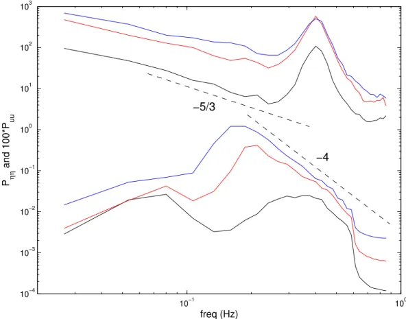
Three episodes in the wave growth process are selected from the data set, each with 213 points. The episodes are centered at the 10 000th, 20 000th, and 48 000th points, respectively, of the data set such that the length of each episode is approx-imately 1.33 h based on a sampling frequency of 1.7 Hz. The mean values of the wind and wave series of each episode are removed, and therefore the remaining parts are wind fluctu-ations, including the wave-induced components and the pure wind turbulence, and the zero-mean wave elevation. The wind and the wave power spectra are estimated by further di-viding the associated episodes into 27(=128) segments and averaging. Figure 1 shows the three pairs of wind and wave power spectra,PuuandPηη, for the three episodes. The
re-sults in Fig. 1 are similar to those in Figs. 2 and 3 of Ge and Liu (2007), but they are different primarily in the length of the episodes and the number of segments used for aver-aging, and hence the frequency resolution. It is evident in Fig. 1 that the−4-power equilibrium range (Phillips, 1985) initially forms in episode 1 overf from 0.4 Hz to 0.6 Hz, and gradually expands to a much lower frequency, approxi-mately 0.2 Hz, in episode 3. The lower end of the equilibrium range forms a spectral peak in both episodes 2 and 3 around 0.2 Hz. This peak will be referred to as the primary peak of the wave spectrum hereafter. Although the growth time from episode 1 to episode 2 is much shorter than that between the last two episodes, the wave spectrum appears to grow much faster between the first two episodes. Besides the ev-ident−5/3-power inertial subrange in the wind fluctuations, the wind power spectrum also varies faster from episode 1 to episode 2. The large peak at aboutf=0.4 Hz, which is interpreted as the primary wave-induced wind component, reaches saturation after episode 2. Unlike the downshifting primary peak of the waves, this primary wind spectral peak stays at 0.4 Hz throughout the data set and appears to be at-tenuated during the last two episodes.
10−1 100 10−4
10−3 10−2 10−1 100 101 102 103
P ηη
and 100*P
uu
freq (Hz)
−4
−5/3
Fig. 1. Wind and wave power spectra for three representative episodes, each with 213 points. Curves on the top: wind spectra; curves on the bottom: wave spectra; black: episode 1 (centered at the 10 000th point); red: episode 2 (centered at the 20 000th point); blue: episode 3 (centered at the 48 000th point).
as strong as the primary peak at 0.4 Hz. Unlike the primary peak, however, the growth of this spectral peak appears to slow down and, in episode 3, this peak is completely flat-tened. One may postulate that the energy of this transient spectral peak is being consumed to support the growth of the primary peak through nonlinear wave-wave interactions. This spectral peak also can be viewed as a swell, because it is at low frequencies around 0.06–0.08 Hz (Kinsman, 2002, p. 22) and it exists even at the initial stage. However, whether this peak reveals a swell will not affect any of the following discussions. Another characteristic is in the wind spectra. Around the joint of the primary wave-induced spectral peak (at about 0.4 Hz) and the turbulence range (the−5/3-power range from approximately 0.06 Hz to the lower bound of the primary wave-induced peak) there is a little bump in all the three episodes. Initially, the bump is at a little higher than 0.2 Hz, and it moves to about 0.2 Hz in episode 2, and it fur-ther moves down to 0.18 Hz in episode 3. A close inspection of this bump suggests that this small spectral peak coincides with the tip (i.e. maximum) of the primary spectral peak of the waves, an interesting property of the wind field.
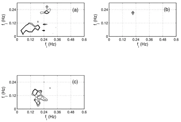
Figure 2 shows the auto-bispectra of the waves in the three episodes for the quadratic wave-wave interaction. First of all, we have the impression that the nonlinear interaction patterns, which potentially will facilitate significant energy transfer between wave components, are very different for the three episodes. In the second episode, for example, only one coupling pattern is evident, indicated by large bispectrum values centered at (0.2, 0.2). In the other two episodes, the nonlinear interactions are much more active and cover wider frequency ranges. We are not going to list all the detected couplings in detail here, for all significant wave-wave inter-actions shown in Fig. 2 will be summarized in Fig. 7. More discussion will be given later.
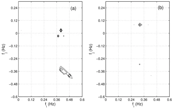
Nonlinear wind-wave interactions for the three episodes are given in Figs. 3 to 5, with the cross-bispectrum Bηηu
shown in (a) andBuuη shown in (b). As defined by Eq. (6),
the cross-bispectrumBηηu quantifies the nonlinear
interac-tion between two wave components that contributes to a third wind component, andBuuηis determined by two wind
0 0.12 0.24 0.36 0.48 0.6 0
0.12 0.24
fi (Hz)
f j
(Hz)
0 0.12 0.24 0.36 0.48 0.6
0 0.12 0.24
fi (Hz)
f j
(Hz)
0 0.12 0.24 0.36 0.48 0.6
0 0.12 0.24
fi (Hz)
f j
(Hz)
(a)
(b)
(c)
Fig. 2. Auto-bispectrum of the wavesBηηη:(a)episode 1;(b)episode 2;(c)episode 3; three contours are shown for each subplot at the
levels of 0.5, 0.7, and 0.9 times the respective maximumBηηη.
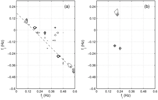
explained by most existing theoretical or numerical mod-els, whose wind-wave interaction components are primar-ily linear. The most evident characteristic in Figs. 3 to 5 is the variability of the coupling patterns revealed byBηηu.
More specifically, an increasing number of components be-come nonlinearly coupled with each other in the waves and their sum/difference components in the winds. Especially in episode 3, many contours indicating high-level quadratic couplings are lined up along a straight line with an invariant sum/difference of approximately 0.18 Hz, i.e. the intercept of the line with thefi-axis. This means that these pairs of
fre-quency components of the wave field, (fi,fj), all contribute
to the same frequency component, 0.18 Hz, in the wind fluc-tuations, a new and prominent pattern compared with those in episodes 1 and 2. This frequency component, at around 0.18 Hz in the wind spectrum, is exactly the small peak that downshifts with the primary peak of the waves (Fig. 1). In contrast, the nonlinear couplings indicated byBuuη are not
so active as those byBηηu.
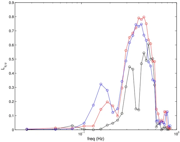
With the growth of the wind-generated wave field, the lin-ear coherence grows at the same time, which is cllin-early shown in Fig. 6. During episode 1, there are two peaks (separated by a valley at about 0.4 Hz) in the linear coherence in the range from 0.3 to 0.6 Hz at the level of 0.4. These peaks of linear coherence experience a rapid growth from episodes 1 to 2, merging and reaching a level of 0.8 over a broad-ened frequency range from 0.23 Hz to 0.6 Hz. Although the
0 0.12 0.24 0.36 0.48 0.6 −0.6
−0.48 −0.36 −0.24 −0.12 0 0.12 0.24
f
i (Hz)
f j
(Hz)
0 0.12 0.24 0.36 0.48 0.6
−0.6 −0.48 −0.36 −0.24 −0.12 0 0.12 0.24
f
i (Hz)
f j
(Hz)
(a)
(b)
Fig. 3.Cross-bispectrum of the waves and the wind fluctuations for episode 1:(a)Bηηu;(b)Buuη; three contours are shown for each subplot
at the levels of 0.5, 0.7, and 0.9 times the respective maximum cross-bispectra.
0 0.12 0.24 0.36 0.48 0.6
−0.6 −0.48 −0.36 −0.24 −0.12 0 0.12 0.24
f
i (Hz)
f j
(Hz)
0 0.12 0.24 0.36 0.48 0.6
−0.6 −0.48 −0.36 −0.24 −0.12 0 0.12 0.24
f
i (Hz)
f j
(Hz)
(a)
(b)
Fig. 4.Same as Fig. 3 but for episode 2.
spectrum. This observation suggests that the bump of the wind spectrum and its downshifting are the signature of the movement of the primary wave peak, where the linear inter-action plays an important role in inducing the corresponding
0 0.12 0.24 0.36 0.48 0.6 −0.6
−0.48 −0.36 −0.24 −0.12 0 0.12 0.24
f
i (Hz)
f j
(Hz)
0 0.12 0.24 0.36 0.48 0.6
−0.6 −0.48 −0.36 −0.24 −0.12 0 0.12 0.24
f
i (Hz)
f j
(Hz)
(a) (b)
Fig. 5.Same as Fig. 3 but for episode 3. All frequency pairs (fi,fj) on the dashed line in(a)have an invariant sum/difference of 0.18 Hz.
based on their different induced components in the wind fluc-tuations through different linear interactions. This property was not revealed by Ge and Liu (2007) using the wavelet-based analyses over short times. Moreover, the statement that the winds’ spectral peak at around 0.4 Hz is induced by the primary peak of the waves based on limited cases over very short times (Ge and Liu, 2007) should be refined accordingly. The major linear and nonlinear couplings that have been detected above are all illustrated in Figs. 7 and 8. For clar-ity, not all interacting components are shown. For the non-linear wind-wave interactions, the arrows in Figs. 7 and 8 do not necessarily indicate the directions of interactions, but always point to the sum/difference components in the cor-responding nonlinear interactions. For the nonlinear wave-wave interactions (Fig. 7), the interacting wave-wave components are marked by open circles and their sum/difference compo-nents are marked by filled circles. Again, the symbols do not imply the directions of interactions, while the wave-wave in-teractions may really be viewed as potential (second-order) energy transfers in the wave field.
Figure 7 shows that in the course of the wave growth both linear and quadratic wind-wave interactions become more and more active. During the first episode, when the pri-mary peak of the wave spectrum has not well formed and the swell component around 0.07 Hz is still energetic, the major feature appears to be a wide range of wave compo-nents coupled with each other through quadratic wave-wave interactions. Almost all wave components, from very low frequencies to high frequencies, are coupled through one or more quadratic interactions, which may result in an
10−1 100 0
0.1 0.2 0.3 0.4 0.5 0.6 0.7 0.8 0.9
L η
u
freq (Hz)
Fig. 6.Linear coherenceLηuof the waves and the wind fluctuations: black: episode 1; red: episode 2; blue: episode 3.
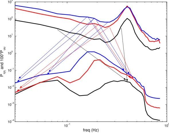
Among other characteristics that Fig. 8 illustrates, it can be observed that in episodes 2 and 3 the small wave-induced component of the winds actively reacts to the wave field, from the low-frequency end (approximately 0.03 Hz) to the equilibrium range around 0.4 Hz. In contrast, the primary wave-induced component of the winds does not have signif-icant feedback to the wave field, except for one quadratic interaction in episode 1. This observation also suggests that the pure wind turbulence does not have persistent influence on the wave growth process or only functions intermittently (Ge and Liu, 2007), consistent with the assumptions of Miles (1957).
It should be pointed out here that the signal processing techniques employed in the present work are up to sec-ond order, while higher order wave-wave interactions have been found to be more important than the second-order ones. Hence, there might be more significant interaction patterns behind the wave growth that we cannot sense from the data. However, fortunately, this limitation is only for the wave-wave interaction, which is typically weak up to the second order. In the presence of an overlying turbulent wind field, the wind-wave interaction is often of first-order significance. Since most findings illustrated in Figs. 7 and 8 are for wind-wave interaction patterns, those results, linear and quadratic,
are adequate to cover major characteristics of the growth of the wind-generated wave field. Modification might be due for the wave-wave interaction patterns when higher-order spectral moments, such as the trispectrum, are used to de-tect third-order couplings (Liu, 1979). For the present case, the use of the trispectrum may add more features to the wave-wave interactions (Figs. 2 and 7), but it will not alter the de-tected general wind-wave coupling characteristics.
5 Conclusions
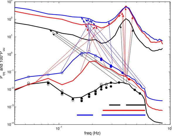
10−1 100 10−4
10−3 10−2 10−1 100 101 102 103
P ηη
and 100*P
uu
freq (Hz)
Fig. 7. Summary of the linear wind-wave interactionsLηu, quadratic wind-wave interactionsBηηu, and quadratic wave-wave interactions
Bηηηfor the three episodes as identified to be significant in Figs. 2–6: black: episode 1; red: episode 2; blue: episode 3; for quadratic
wave-wave interactions, the interacting wave-wave components are represented by open circles and their corresponding sum/difference components are represented by filled circles; arrows start from interacting wave components and point to their corresponding sum/difference components in the wind fluctuations; for clarity, not all interacting components are shown; heavy horizontal lines on the bottom show frequency ranges for significant linear coherence.
concentrated on studying the effects of the wind fluctuations, including the wave-induced components and the wind turbu-lence, on the growth of the wave field and the feedback they receive at the same time.
Similar to those shown by Ge and Liu (2007), the wind and wave power spectra exhibit some special properties of the data set, such as the merging of the primary peak and the equilibrium range of the wave spectrum, a low frequency wave peak that could be interpreted as a swell, and a strongly induced wind component over the same frequency range as the equilibrium range of the wave spectrum. For this par-ticular case, the use of the Fourier-domain analyses allows for detection of long-term linear and quadratic phase cou-plings between the wind fluctuations and the waves. The re-sults show that both the frequency range and the strength of the linear interactions tend to be broadened and enhanced at pace with the growing waves. The linear coupling is found to be an effective and important mechanism especially for the generation of the wave-induced wind components
10−1 100 10−4
10−3 10−2 10−1 100 101 102 103
P ηη
and 100*P
uu
freq (Hz)
Fig. 8.Summary of the quadratic wind-wave interactionsBuuηas identified to be significant in Figs. 3–5: arrows start from interacting wind
components and point to their corresponding sum/difference components in the waves; for clarity, not all interacting components are shown.
generated from the second episode through quadratic interac-tions with wave components in a large frequency range (from 0.06 Hz to 0.4 Hz in episode 2 and from 0.1 Hz to 0.6 Hz in episode 3). At the same time, this small peak of the winds moves to lower frequencies together with the downshifting of the primary wave peak through linear interactions. These two wave-induced wind components are thus distinct due to their different behaviour and different interaction patterns with the wave field. Thirdly, the saturation of the primary wave-induced component of the winds (around 0.4 Hz) dur-ing episode 3 coincides with the observation that no wave components are quadratically coupled with this wind compo-nent, although the local linear interactions are still at work. Lastly, the small wave-induced peak in the winds (around 0.2 Hz) appears to be active in quadratic coupling with its sideband (i.e. its adjacent components) and their associated sum/difference components in the wave field, while the pri-mary wave-induced component of the winds (around 0.4 Hz) does not seem to have such a feedback. This also reveals weak and intermittent influence of the wind turbulence on the wave field.
All the coupling patterns, especially the nonlinear wind-wave interactions, detected above cannot be readily
ex-plained or predicted by the existing theories or numerical models. This work consequently could be beneficial for fu-ture model development and validation.
Acknowledgements. This work was partially supported by the Re-search Associateship Programs of the National ReRe-search Council. The authors also wish to thank W. Frick of USEPA for his helpful advice.
Topical Editor S. Gulev thanks A. Babanin and another anony-mous referee for their help in evaluating this paper.
Disclaimer. This paper has been reviewed in accordance with the US Environmental Protection Agency’s peer and administrative re-view policies and approved for publication. Mention of trade names or commercial products does not constitute endorsement or recom-mendation for use.
References
Belcher, S. E. and Hunt, J. C. R.: Turbulent flow over hills and waves, Annu. Rev. Fluid Mech., 30, 507–538, 1998.
Burgers, G. B. and Makin, V. K.: Boundary-layer model results for wind-sea growth, J. Phys. Oceanogr., 23, 372–385, 1993. Donelan, M. A., Babanin, A. V., Young, I. R., and Banner, M.
spec-tral function. Part II: Parameterization of the wind input, J. Phys. Oceanogr., 36, 1672–1689, 2006.
Ge, Z. and Liu, P. C.: A time-localized response of wave growth process under turbulent winds, Ann. Geophys., 25, 1253–1262, 2007,
http://www.ann-geophys.net/25/1253/2007/.
Gilhousen, D. B.: A field evaluation of NDBC moored buoy winds, J. Atmos. Ocean Tech., 4, 94–104, 1987.
Gilhousen, D. B.: A complete explanation of why moored buoy winds are less than ship winds, Mariners Weather Log, 50, 1, National Oceanic and Atmospheric Administration, April 2006. Hajj, M. R., Miksad, R. W., and Powers, E. J.: Perspective:
Measurements and analyses of nonlinear wave interactions with higher-order spectral moments, J. Fluids Eng., 119, 3–13, 1997. Hasselmann, K.: On the non-linear energy transfer in a
gravity-wave spectrum. Part 1. General theory, J. Fluid Mech., 12, 481– 500, 1962.
Hasselmann, K.: On the non-linear energy transfer in a gravity-wave spectrum. Part 3. Evaluation of the energy flux and swell-sea interaction for a Neumann spectrum, J. Fluid Mech., 15, 385– 398, 1963.
Herbers, T. H. C. and Guza, R. T.: Wind-wave nonlinearity ob-served at the sea floor. Part I: Forced-wave energy, J. Phys. Oceanogr., 21, 1740–1761, 1991.
Herbers, T. H. C. and Guza, R. T.: Wind-wave nonlinearity ob-served at the sea floor. Part II: Wavenumbers and third-order statistics, J. Phys. Oceanogr., 22, 489–504, 1992.
Janssen, P. A. E. M.: Quasi-linear theory of wind-wave generation applied to wave forecasting, J. Phys. Oceanogr., 21, 1631–1642, 1991.
Kinsman, B.: Wind waves: Their generation and propagation on the ocean surface, Dovers Publications, Inc., Mineola, New York, NY, 2002.
Koman, G. J.: Nonlinear contributions to the frequency spectrum of wind-generated waves, J. Phys. Oceanogr., 10, 779–790, 1980.
Komen, G. J., Cavaleri, L., Donelan, M., Hasselmann, K., Hassel-mann, S., and Janssen, P. A. E. M.: Dynamics and modelling of ocean waves, Cambridge University Press, New York, NY, 1994. Lavrenov, I. V.: Wind-waves in oceans: Dynamics and numerical
simulations, Springer-Verlag, 2003.
Liu, P. C.: Spectral growth and nonlinear characteristics of wind waves in Lake Ontario, NOAA Technical Report ERL 408-GLERL 14, November 1979.
Miles, J. W.: On the generation of surface waves by shear flows, J. Fluid Mech., 3, 185–204, 1957.
Phillips, O. M.: On the generation of waves by turbulent wind, J. Fluid Mech., 2, 417–445, 1957.
Phillips, O. M: Nonlinear dispersive waves, Annu. Rev. Fluid Mech., 6, 93–110, 1974.
Phillips, O. M.: Spectral and statistical properties of the equilibrium range in wind-generated gravity waves, J. Fluid Mech., 156, 505– 531, 1985.
Ritz, C. P. and Powers, E. J.: Estimation of nonlinear transfer func-tions for fully developed turbulence, Physica D., 20, 320–334, 1986.
Ritz, C. P., Powers, E. J., Miksad, R. W., and Solis, R. S.: Nonlinear spectral dynamics of a transitioning flow, Phys. Fluids, 31, 3577– 3588, 1988.
Ritz, C. P., Powers, E. J., and Bengtson, R. D.: Experimental mea-surement of three-wave coupling and energy cascading, Phys. Fluids B., 1, 153–163, 1989.
Tolman, H. L. and Chalikov, D.: Source terms in a third-generation wind wave model, J. Phys. Oceanogr., 26, 2497–2518, 1996. Weller, R. A., Donelan, M. A., Briscoe, M. G., and Huang, N. E.: