Nanofluid Flow past an Unsteady Permeable Shrinking Sheet
with Heat Source or Sink and Newtonian Heating in a Porous
Medium
M.Lavanya
1, Dr. M.Sreedhar Babu
2, G. Venkata Ramanaiah
3Research scholar, Dept. of Applied Mathematics, Y.V.University, Kadapa Andhra Pradesh, India. Asst.professor, Dept. of Applied Mathematics, Y.V.University, Kadapa Andhra Pradesh, India. Research scholar, Dept. of Applied Mathematics, Y.V.University, Kadapa Andhra Pradesh, India.
ABSTRACT
The consideration of nanofluids has been paid a good attention on the forced convection; the analysis focusing nanofluids in porous media are limited in literature. Thus, the use of nanofluids in porous media would be very much helpful in heat and mass transfer enhancement. In this paper, the influence of variable suction, Newtonian heating and heat source or sink heat and mass transfer over a permeable shrinking sheet embedded in a porous medium filled with a nanofluid is discussed in detail. The solutions of the nonlinear equations governing the velocɨty, temperature and concentration profiles are solved numerically using Runge-Kutta Gill procedure together with shooting method and graphical results for the resulting parameters are displayed and discussed. The influence of the physical parameters on skin-friction coefficient, local Nusselt number and local Sherwood number are shown in a tabulated form.
Keywords
: nanofluid, Newtonian heating, heat generation/absorption, Shrinking sheet, wall mass suction.I.
INTRODUCTION
For industrial application the heat transfer phenomena in boundary layer flow on a stretching or shrinking sheet is of great importance. Crane (1970) first studied the flow due to a linear stretching plate. The heat transfer in boundary layer flow of Maxwell fluid over a porous shrinking sheet with wall mass transfer is investigated by Bhattacharyya et al. (2013). They revealed that the viscous boundary layer thickness reduces with Deborah number.
The influence of internal heat generation in a problem reveals that it affects the temperature distribution strongly. Internal heat generation is related in the fields of disposal of nuclear waste, storage of radioactive materials, nuclear reactors safely analysis, fire and combustion studies and in many industrial processes. Consideration of internal heat generation becomes a key factor in many engineering applications. Heat generation can be assumed to be constant or space temperature dependent. Crepeau and Clarksean (1997) applied a space dependent heat generation in their study on flow and heat transfer from vertical plate. They observed that the exponentially decaying heat generation model can be used in mixtures where a radioactive material is surrounded by inert alloys. Makinde (2011) computed similarity solutions for natural convection from a moving vertical plate with internal heat generation. It was found that an increase in the exponentially decaying internal heat generation causes a further increase in both velocity and thermal boundary layer thicknesses. Ganga et al (2015) studied the effects of internal heat generation or absorption on magnetohydrodynamic and radiative boundary layer flow of nanofluid over a vertical plate with viscous and ohmic dissipation.
The study of stretched flows with heat transfer is given a much importance. The heat transfer is through constant wall temperature or constant wall heat flux. Also there are another class of flow problems in which the rate of heat transfer is proporsional to the local surface temperature from the boundary surface with finite heat capacity known as Newtonian heating or conjugate convective flow. The boundary layer natural convective flow with Newtonian heating is studied by Merkin (1994). Chaudhary et al. (2007) observed the similarity solution for unsteady free convection flow past on impulsive vertical surface in the presence of Newtonian heating.
In this paper, we have study the phenomenon of unsteady forced convection in Newtonian heating under the application of uniform porous medium when heat generation or absorption appears in the energy equation in the flow of a nanofluid. The flow is induced by a permeable shrinking sheet. The solutions of the nonlinear equations governing the velocɨty, temperature and concentration profiles are solved numerically using Runge-Kutta Gill procedure together with shooting method and graphical results for the resulting parameters are
www.ijera.com
displayed and discussed. The influence of the physical parameters on skin-friction coefficient, local Nusselt number and local Sherwood number are shown in a tabulated form.
II.
MATHEMATICAL FORMULATION
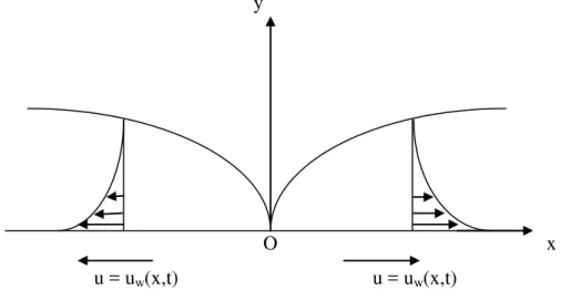
Unsteady, two dimensional, forced convection boundary layer flow past a permeable shrinking sheet is considered. The sheet is embedded in a porous medium filled with a nanofluid in the presence of internal heat generation or absorption and Newtonian heating. The schematic diagram for the present flow model is illustrated in figure A.
y
O x
u = u
w(x,t) u = u
w(x,t)
Figure A: Schematic diagram of the physical configuration and coordinate system.
It is assumed that the velocity of the shrinking sheet is
u
w
x t
,
and the velocity of the mass transfer is
,
w
v
x t
, where x is the coordinate measured along the shrinking sheet and t is the time. The standardized wall temperature of the sheet Tw and standardized nanoparticle volume fraction Cw are unspoken to be superior to the ambient temperature T ͚ and ambient nanoparticle volume fraction C, respectively.With the usual Boussinesq and the boundary layer approximations, the governing equations of continuity, momentum, energy and species are written as follows
� � +
�
� = 0 (2.1) �
� + � � +
� � =
�2
� 2−�′
(2.2)
�� � +
�� � +
�� � =��
�2�
� 2+
�� �
�� � +
�
�∞
�� �
2
+ 0
��� (� − �∞) (2.3)
� � +
� � +
� � = �
�2
� 2+
�
�∞
�2�
� 2 (2.4)
The appropriate boundary conditions for the flow model are written as follows
( , )
,
( , ),
,
1
w w c s
cx
T
C
u
u
x t
v
v x t
h T
h C
t
y
y
aty
'
0
0,
,
u
T
T C
C
asy
'
(2.5) where u and v are the velocity components in the x-direction and y-direction respectively, be kinematic viscosity, hc be heat transfer coefficient, hs is mass transfer coefficient, k′ be permeability of the porous medium constant, q0 be heat generation or absorption coefficient, beelectrical conductivity (assumed constant), ρf be density of the base fluid, �m be thermal diffusivity, DB be Brownian diffusion coefficient, DT be thermophoresis diffusion coefficient and cp be specific heat at constant pressure. Here is the ratio of nanoparticle heat capacity and the base fluid heat capacity, T is variable temperature and C is local nanoparticle volume fraction.The wall mass transfer velocity then becomes
,
1
w
c
v
x t
S
t
where S is the constant wall mass transfer parameter with S > 0 for suction and S < 0 for injection, respectively. The equation of continuity is satisfied for the choice of a stream function
( , )
x y
such thaty
u
and
v
x
(2.7)
In order to transform the equations (2.2) to (2.5) into a set of ordinary differential equations, the following similarity transformations and dimensionless variables are introduced.
0,
,
,
1
1
(
)
'
,
, Pr
,
,
,
1
1
(
)
,
,
,
w w
B w
m f p
T w
c s
B
c
c
T
T
C C
xf x
y
t
t
T
T
C
C
D C
C
q
k c
K
A
Nb
Q
c
c c
t
t
D T
T
Nt
Le
h
h
T
D
c
c
(2.8)where
f
be dimensionless stream function,
be dimensionless temperature,
be dimensionless concentration,
be similarity variable, K be local permeability parameter, A be local unsteadiness parameter, Pr be local Prandtl number, Nb be local Brownian motion parameter, Nt be local thermophoresis parameter, Le be local Lewis number, Q be local heat generation or absorption parameter, be local conjugate parameter for Newtonian heating and
be local conjugate parameter for concentration.After the substitution of these transformations (2.8) along with the equation (2.7) into the Equations (2.2)-(2.6), the resulting non-linear ordinary differential equations are written as
2
1
'''
''
'
'
''
'
0
2
f
ff
f
A f
f
f
K
(2.9)2
1
"
'
'
' '
'
0
Pr
f
A
2
Nb
Nt
Q
(2.10)"
'
''
0
2
Nt
Le f
A
Nb
(2.11) The transformed boundary conditions can be written as
(0)
,
'(0)
1, '(0)
1
(0) , '(0)
1
(0)
f
S f
'
0,
0,
0
f
as
(2.12) where primes denote differentiation with respect to �Physical quantities of interest are Local skin friction coefficient
C
f , the heat transfer rate and masstransfer rate are the main physical characteristics of the problem, which are described in terms of local Nusselt number and local Sherwood number, respectively, defined as
2
,
,
w w m
fx x x
f w w B w
xq
xq
C
Nu
Sh
u
k T
T
D
C
C
(2.13) where
xy is the shear stress at the stretching sheet,q
w andq
mis the heat and mass flux, respectively.Thus, we get
1/ 2 1 2 1 2Re
''(0)
Re
' 0
Re
' 0
x f x x x x
C
f
Nu
Sh
(2.14)Where
Re
w( , )
xu
x t x
www.ijera.com
III.
SOLUTION OF THE PROBLEM
For solving equations (2.9)–(2.11), a step by step integration method i.e. Runge–Kutta method has been applied. For carrying in the numerical integration, the equations are reduced to a set of first order differential equation. For performing this we make the following substitutions:
1 2 3 4 5 6 7
2
3 2 1 3 2 3 2
2
5 5 1 5 5 7 5 4
2
7 1 7 5 1 5 5 7 5 4
,
',
'',
,
',
,
'
1
'
2
'
Pr
2
'
Pr
2
2
y
f y
f
y
f
y
y
y
y
y
y
y y
A y
y
y
K
y
A
y
y y
Nby y
Nty
Qy
Nt
y
Le y
A
y
A
y
y y
Nby y
Nty
Qy
Nb
(3.1) together with the boundary conditions are given by (2.12) taking the form
1 2 5 4 7 6
2 4 6
(0) , (0) 1, (0) 1 (0) , (0) 1 (0)
( ) 0, ( ) 0, ( ) 0
y S y y y y y
y y y
(3.2) In order to carry out the step by step integration of equations (2.9) –(2.11), Gills procedures as given in Ralston and Wilf (1960) have been used. To start the integration it is necessary to provide all the values of
1
,
2,
3,
4,
5,
6y y y y y y
at
0
from which point, the forward integration has been carried out but from the boundary conditions it is seen that the values ofy y y
3,
4,
7 are not known. So we are to provide such values of3
,
4,
7y y y
along with the known values of the other function at
0
as would satisfy the boundary conditions as
to a prescribed accuracy after step by step integrations are performed. Since the values ofy y y
3,
4,
7 which are supplied are merely rough values, some corrections have to be made in these values in order that the boundary conditions to
are satisfied. These corrections in the values ofy y y
3,
4,
7 are taken care of by a self-iterative procedure which can for convenience be called ‘‘Corrective procedure’’.IV.
RESULTS AND DISCUSSION
In order to acquire physical understanding, the velocɨty, temperature & concentration distributions have been illustrated by varying the numerical values of the various parameters demonstrated in the present problem. The numerical results are tabulated and exhibited with the graphical illustration.
Figures 1(a)-1(c) establishes the different values of permeability of the porous medium parameter (K) on velocɨty, temperature and concentration profiles, respectively. The values of K is taken to be K = 0.1, 0.6, 1.2, 2 and the other parameters are fixed as A = -1, σt = 0.1, σb = 0.1, Q = 0.β, = 0.γ, = 0.γ, Le = 1, Pr = 0.7 and S = 2. It is noticed that, with the hype in the values of K from 0.1 to 2.0 then the velocity decreases consequently decreases the thickness of momentum boundary layer but the temperature and concentration of the fluid increases. The reason for this, the porous medium obstructs the fluid to move freely through the boundary layer. This leads to the raise in the thickness of thermal and concentration boundary layer. Figures 2(a)-2(c) establishes the different values of unsteadiness parameter (A) on velocɨty, temperature and concentration profiles, respectively. The values of A is taken to be A = - 1, - 2, - 3, - 4 and the other parameters are fixed as K = 0.5, Nt = 0.1, σb = 0.1, Q = 0.β, = 0.γ, = 0.γ, Le = 1, Pr = 0.7 and S = β. It is noticed that, with the hype in the values of A from -4 to -1 then the velocity, temperature and concentration profiles increases consequently enhanced the thickness of momentum, thermal and concentration boundary layer.
The velocɨty, temperature and concentration distributions for suction parameter S are illustrated in Figures 3(a) -3(c). The values of S is taken to be S = 2, 3, 4, 5 and the other parameters are fixed as A = -1, K = 0.5, Nt = 0.1, σb = 0.1, Q = 0.β, = 0.γ, = 0.γ, Le = 1 and Pr = 0.7. It can be viewed that suction will lead to fast cooling of the surface. This is remarkably important in numerous industrial applications. It is observed that the velocity, temperature and concentration diminish with raising the values of S. This results in a reduction in the thickness of momentum, thermal and concentration boundary layers.
enhance the thickness of thermal and concèntration boundary layer. The effect of Brownian motion parameter (Nb) on the temperature and concentration fields is illustrated in figures 5(a) & 5(b) respectively. The values of Nb is taken to be Nb = 0.1, 0.3, 0.5, 0.8 and the other parameters are fixed as A = -1, K = 0.5, Nt = 0.1, Q = 0.2, = 0.γ, = 0.γ, Le = 1, Pr = 0.7 and S = β. It is conformed that enhances the values of Nb from 0.1 to 0.8, the temperature profile increases but concentration decreases. In the system nanofluid, the Brownian motion takes a place in the presence of nànoparticles. When hype the values of Nb, the Brownian motion is affected and the concèntration boundary layer thickness reduces and accordingly the heat transfer characteristics of the fluid changes.
The effect of heat generation or absorption parameter (Q) on temperature and concentration fields is depicted in figures 6(a) and 6(b), respectively. The values of Q is taken to be Q = - 0.5, - 0.2, 0, 0.2, 0.5 and the other parameters are fixed as A = -1, K = 0.5, σt = 0.1, σb = 0.1, = 0.γ, = 0.γ, Le = 1, Pr = 0.7 and S = β. It is observed that the thickness of thermal and concentration boundary layer increases with raising the values of δ from -0.5 to 0.5. Figures 7(a) and 7(b) depicts the various values of conjugate parameter for Newtonian heating ( ) on the temperature and concentration profiles, respectively. The values of is taken to be = 0.1, 0.β, 0.γ, 0.4 and the other parameters are fixed as A = -1, K = 0.5, σt = 0.1, σb = 0.1, Q = 0.β, = 0.γ, Le = 1, Pr = 0.7 and S = 2. It can be understood that raising the values of from 0.1 to 0.4 the resultant temperature and concentration increases consequently thickness of thermal and concèntration boundary layer enhances.
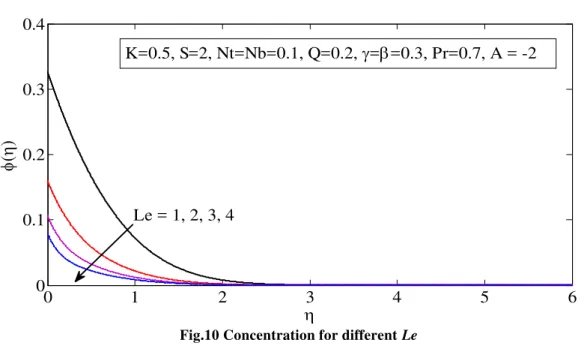
Figures 8(a) and 8(b) depicts the various values of conjugate parameter for concentration ( ) on the temperature and concentration fields, respectively. The values of is taken to be = 0.1, 0.5, 0.8, 1 and the other parameters are fixed as A = -1, K = 0.5, σt = 0.1, σb = 0.1, Q = 0.β, = 0.γ, = 0.γ, Le = 1, Pr = 0.7 and S = β. It is obtained that raising the values of from 0.1 to 1.0, the temperature of the fluid increases. This leads to enhance the thermal and concentration boundary layer thickness. The effect of Prandtl number Pr on temperature and concentration fields is shown in figures 9(a) & 9(b) respectively. The values of Pr is taken to be Pr = 1, 2, 3, 4 and the other parameters are fixed as A = -1, K = 0.5, σt = 0.1, σb = 0.1, Q = 0.β, = 0.γ, = 0.γ, Le = 1 and S = 2. Physically, increasing Prandtl number becomes a key factor to reduce the thickness of thermal and nanoparcle concèntration boundary layers. The effect of Lewis number Le verses concentration profile is shown in figure 10 respectively. The values of Le is taken to be Le = 1, 2, 3, 4 and the other parameters are fixed as A = -1, K = 0.5, σt = 0.1, σb = 0.1, Q = 0.β, = 0.γ, = 0.γ, Pr = 0.7 and S = 2. It can be obtained that the concentration of the fluid decreases with raising the values of Le from 1 to 4.
In order to standardize the method used in the present study and to decide the accuracy of the present analysis and to compare with the results available (Khan et al. (2015), Wang (1989), Khan and Pop (2010), and Gorla and Sidawi (1994)) relating to the local skin-friction coefficient in the absence of porous medium and found in an agreement (Table.1).
Table 2 reveals the magnitude of skin fraction on different values of A, S and K. It is noticed that with the raise in values of A from -4 to -1, the resultant values of then
f
''(0)
increases. With the raise in the values of S from 2 to 5, then the resultant values off
''(0)
increases and with the raise in the values of K from 0.5 to 2, then the resultant values off
''(0)
decreases. Table 3 reveals the local Nusselt number and local Sherwood number on different parameters. It is noticed that with the raise in values of A from -4 to -1, then the resultant values of
'(0)
and
'(0)
increases. With the raise in the values of Nt from 0.1 to 0.7, then the resultant values of
'(0)
and
'(0)
increases. With the raise in values of Nb from 0.1 to 1.0, the resultant values of
'(0)
increases whereas
'(0)
decreases. With the raise in the values of Q from -0.5 to 0.5, the resultant values of
'(0)
and
'(0)
is to be increases. With the raise in the values of S from 2 to 5, the resultant values of
'(0)
and
'(0)
is to be decreases. With the raise in the values of Le from 1 to 4, the resultant values of
'(0)
and
'(0)
is to be decreases. With the raise in the values of Pr from 0.7 to 3, the resultant values of
'(0)
and
'(0)
is to be decreases. With the raise in the values of K from 0.5 to 2, the resultant values of
'(0)
and
'(0)
is to be increases. With the raise in the values of from 0.1 to 1.0, the resultant values of
'(0)
and
'(0)
is to be increases. Finally, with the raise in the values of from 0.1 to1, the resultant values of
'(0)
and
'(0)
is to be increases.V.
CONCLUSIONS
www.ijera.com
1. Thickness of velocity, temperature and concentration boundary layer decreases with a rising the values of mass suction parameter.
2. Velocity decreases whereas temperature and concentration increases with increases the values of permeability parameter and unsteadiness parameter.
3. Temperature and concentration increases with an increase thermophoresis parameter, heat generation or absorption parameter, conjugate parameter for Newtonian heating and conjugate parameter for concentration. Temperature increases and concentration decreases with an increase Brownian motion parameter.
4. Skin-friction coefficient increases with increases the values of suction parameter and unsteadiness parameter and opposite results were found in permeability parameter.
5. Local Nusselt number and local Sherwood number increases with increases thermophoresis parameter, heat generation or absorption parameter, conjugate parameter for Newtonian heating and conjugate parameter for concentration whereas it decrease with raising the values of suction parameter, Lewis number and Prandtl number.
6. Local Nusselt number increases but local Sherwood number decreases with increasing the values of Brownian motion parameter.
Fig. 1(a) Velocity for different K
0
1
2
3
4
5
-1
-0.8
-0.6
-0.4
-0.2
0
f '
(
)
Fig. 1(b) Temperature for different K
Fig. 1(c) Concentration for different K
0
1
2
3
4
5
0
0.05
0.1
0.15
0.2
0.25
0.3
(
)
A = -1, Nt=Nb=0.1, Q=0.2,
=
=0.3, Le=1, Pr=0.7, S =2
K = 0.1, 0.6, 1.2, 2
0
1
2
3
4
5
0
0.05
0.1
0.15
0.2
0.25
0.3
0.35
0.4
(
)
K = 0.1, 0.6, 1.2, 2
www.ijera.com Fig. 2(a) Velocity for different A
Fig.2(a) Temperature for different A
Fig.2(c) Concentration for different A
0 0.5 1 1.5 2 2.5 3 3.5 4
-1 -0.8 -0.6 -0.4 -0.2 0
f '
(
)
A = -1, -2, -3, -4
K=0.5, Nt=Nb=0.1, Q=0.2, ==0.3, Le=1, Pr=0.7, S =2
0 1 2 3 4 5
0 0.05 0.1 0.15 0.2 0.25
(
)
K = 0.5, Nt=Nb=0.1, Q=0.2, ==0.3, Le=1, Pr=0.7, S =2
A = -1, -2, -3, -4
0
1
2
3
4
5
0
0.05
0.1
0.15
0.2
0.25
0.3
0.35
(
)
A = -1, -2, -3, -4
Fig.3(a) Velocity for different S
Fig.3(b) Temperature for different S
Fig.3(c) Concentration for different S
0
1
2
3
4
5
-1
-0.8
-0.6
-0.4
-0.2
0
f '
(
)
S = 2, 3, 4, 5
K=0.5, Nt=Nb=0.1, Q=0.2, ==0.3, Le=1, Pr=0.7, A =-2
0
0.5
1
1.5
2
2.5
3
3.5
4
0
0.05
0.1
0.15
0.2
0.25
(
)
S = 2, 3, 4, 5
K = 0.5, Nt=Nb=0.1, Q=0.2, ==0.3, Le=1, Pr=0.7, A =-2
0 0.5 1 1.5 2 2.5 3 3.5 4
0 0.05 0.1 0.15 0.2 0.25 0.3
(
)
S = 2, 3, 4, 5
www.ijera.com Fig.4(a) Temperature for different Nt
Fig.4(b) Concentration for different Nt
Fig.5(a) Temperature for different Nb
0
2
4
6
8
10
0
0.2
0.4
0.6
0.8
1
(
)
Nt = 0.1, 0.3, 0.5, 0.8
K = 0.5, S=2, Nb=0.1, Q=0.2, ==0.3, Le=1, Pr=0.7, A =-2
0 2 4 6 8 10
0 0.5 1 1.5 2 2.5 3
(
)
K=0.5, S=2, Nb=0.1, Q=0.2, ==0.3, Le=1, Pr=0.7, A = -2
Nt = 0.1, 0.3, 0.5, 0.8
0 1 2 3 4 5 6
0 0.1 0.2 0.3 0.4 0.5 0.6
(
)
Nb = 0.1, 0.3, 0.5, 0.8
Fig.5(b) Concentration for different Nb
Fig.6(a) Temperature for different Q
Fig.6(b) Concentration for different Q
0 1 2 3 4 5 6
0 0.1 0.2 0.3 0.4 0.5 0.6
(
)
K=0.5, S=2, Nt=0.1, Q=0.2, ==0.3, Le=1, Pr=0.7, A = -2
Nb = 0.1, 0.3, 0.5, 0.8
0
2
4
6
8
10
0
0.2
0.4
0.6
0.8
(
)
Q = -0.5, -0.2, 0, 0.2, 0.5
K = 0.5, S=2, Nt=Nb=0.1, ==0.3, Le=1, Pr=0.7, A =-2
0
1
2
3
4
5
6
0
0.1
0.2
0.3
0.4
0.5
0.6
(
)
Q = -0.5, -0.2, 0, 0.2, 0.5
www.ijera.com Fig.7(a) Temperature for different Ȗ
Fig.7(b) Concentration for different Ȗ
Fig.8(a) Temperature for different ȕ
0 1 2 3 4 5 6
0 0.2 0.4 0.6 0.8 1
(
)
= 0.1, 0.2, 0.3, 0.4
K = 0.5, S=2, Nt=Nb=0.1, Q=0.2, =0.3, Le=1, Pr=0.7, A =-2
0
1
2
3
4
5
6
0
0.2
0.4
0.6
0.8
1
(
)
= 0.1, 0.2, 0.3, 0.4
K=0.5, S=2, Nt=Nb=0.1, Q=0.2, =0.3, Le=1, Pr=0.7, A = -2
0
1
2
3
4
5
6
0
0.2
0.4
0.6
0.8
(
)
= 0.1, 0.5, 0.8, 1
Fig.8(b) Concentration for different ȕ
Fig.9(a) Temperature for different Pr
Fig.9(b) Concentration for different Pr
0
1
2
3
4
5
6
0
1
2
3
4
5
(
)
= 0.1, 0.5, 0.8, 1
K=0.5, S=2, Nt=Nb=0.1, Q=0.2, =0.3, Le=1, Pr=0.7, A = -2
0 0.5 1 1.5 2 2.5 3 3.5 4
0 0.05 0.1 0.15 0.2
(
)
Pr = 1, 2, 3, 4
K = 0.5, S=2, Nt=Nb=0.1, Q=0.2, ==0.3, Le=1, A =-2
0 0.5 1 1.5 2 2.5 3 3.5 4
0 0.05 0.1 0.15 0.2 0.25 0.3
(
)
Pr = 1, 2, 3, 4
www.ijera.com Fig.10 Concentration for different Le
Table 1. Comparison of the present results of local Nusselt number
'(0)
for Nt=Nb=Q= = =Le=A=0 Pr
'(0)
Present Study Khan et al. (2015)
Khan and Pop (2010)
Wang (1989) Gorla and Sidawi (1994) 0.7 2 7 20 0.454470 0.911353 1.895400 3.353902 0.45392 0.91135 1.89543 3.35395 0.4539 0.9113 1.8954 3.3539 0.4539 0.9114 1.8954 3.3539 0.5349 0.9114 1.8905 3.3539
Table 2 Numerical values of
f
''(0)
for various values of A, S and K when Nt=Nb=0.1, Pr=0.7, Le=1,Q=0.β, = =0.γ.
A S K
f
''(0)
-1 -2 -3 -4 2 2 2 2 0.5 0.5 0.5 0.5 2.196829 1.969200 1.732552 1.487845 -2 -2 -2 3 4 5 0.5 0.5 0.5 2.987691 3.993987 4.996660 -2 -2 -2 2 2 2 1.0 1.5 2.0 0.350960 0.324649 0.316211Table 3 Numerical values of
'(0),
'(0)
for various values of A, Nt, Nb, Q, S, Le, Pr, K, and .A Nt Nb Q S Le Pr K
'(0)
'(0)
-1 -2 -3 -4 0.1 0.1 0.1 0.1 0.1 0.1 0.1 0.1 0.2 0.2 0.2 0.2 2 2 2 2 1 1 1 1 0.7 0.7 0.7 0.7 0.5 0.5 0.5 0.5 0.3 0.3 0.3 0.3 0.3 0.3 0.3 0.3 0.388167 0.374842 0.366859 0.361283 0.414886 0.397972 0.387530 0.380142 -2 -2 -2 0.3 0.5 0.7 0.1 0.1 0.1 0.2 0.2 0.2 2 2 2 1 1 1 0.7 0.7 0.7 0.5 0.5 0.5 0.3 0.3 0.3 0.3 0.3 0.3 0.377387 0.380147 0.383156 0.498900 0.600252 0.702108 -2 -2 -2 0.1 0.1 0.1 0.3 0.5 1.0 0.2 0.2 0.2 2 2 2 1 1 1 0.7 0.7 0.7 0.5 0.5 0.5 0.3 0.3 0.3 0.3 0.3 0.3 0.376121 0.377431 0.380852 0.364442 0.357736 0.352707
0
1
2
3
4
5
6
0
0.1
0.2
0.3
0.4
(
)
Le = 1, 2, 3, 4
-2 -2 -2 -2 -2 0.1 0.1 0.1 0.1 0.1 0.1 0.1 0.1 0.1 0.1 -0.5 -0.2 0.0 0.2 0.5 2 2 2 2 2 1 1 1 1 1 0.7 0.7 0.7 0.7 0.7 0.5 0.5 0.5 0.5 0.5 0.3 0.3 0.3 0.3 0.3 0.3 0.3 0.3 0.3 0.3 0.362822 0.367212 0.370717 0.374842 0.382652 0.397501 0.397671 0.397809 0.397972 0.398287 -2 -2 -2 0.1 0.1 0.1 0.1 0.1 0.1 0.2 0.2 0.2 3 4 5 1 1 1 0.7 0.7 0.7 0.5 0.5 0.5 0.3 0.3 0.3 0.3 0.3 0.3 0.347960 0.335184 0.327737 0.365112 0.348472 0.338486 -2 -2 -2 0.1 0.1 0.1 0.1 0.1 0.1 0.2 0.2 0.2 2 2 2 2 3 4 0.7 0.7 0.7 0.5 0.5 0.5 0.3 0.3 0.3 0.3 0.3 0.3 0.374431 0.374263 0.374169 0.348114 0.331861 0.323801 -2 -2 -2 0.1 0.1 0.1 0.1 0.1 0.1 0.2 0.2 0.2 2 2 2 1 1 1 1 2 3 0.5 0.5 0.5 0.3 0.3 0.3 0.3 0.3 0.3 0.350960 0.324649 0.316211 0.397027 0.396188 0.395942 -2 -2 -2 0.1 0.1 0.1 0.1 0.1 0.1 0.2 0.2 0.2 2 2 2 1 1 1 0.7 0.7 0.7 1.0 1.5 2.0 0.3 0.3 0.3 0.3 0.3 0.3 0.376209 0.377042 0.377658 0.399735 0.400808 0.401601 -2 -2 -2 0.1 0.1 0.1 0.1 0.1 0.1 0.2 0.2 0.2 2 2 2 1 1 1 0.7 0.7 0.7 0.5 0.5 0.5 0.6 0.8 1.0 0.3 0.3 0.3 1.014202 1.820552 4.427824 0.483246 0.589735 0.924805 -2 -2 -2 0.1 0.1 0.1 0.1 0.1 0.1 0.2 0.2 0.2 2 2 2 1 1 1 0.7 0.7 0.7 0.5 0.5 0.5 0.3 0.3 0.3 0.5 0.8 1.0 0.375470 0.376777 0.378045 0.741888 1.443634 2.108415
REFERENCES
[1.] Chaudhary RC, Jain P., (2007), an exact solution to the unsteady free convection boundary layer flow past an impulsively started vertical surface with Newtonian heating, J. Engin. phys. Thermophys, Vol.80, pp.954–960.
[2.] Crane L.J., (1970), Flow past a stretching plate, J. Appl. Math. Phys., (ZAMP), Vol.21, pp.645-647. [3.] Crepeau J.C., and Clarksean R, (1997), Similarity solutions of natural convection with internal heat
generation, Journal of heat and mass transfer, Vol.119, No.1, pp.183- 185.
[4.] Ganga, B., Mohamed Yusuff Ansari, S., Vishnu Ganesh, N., Abdul Hakeem, A.K., (2015), MHD radiative boundary layer flow of nanofluid past a vertical plate with internal heat generation/ absorption, viscous and ohmic dissipation effects, Journal of the Nigerian Mathematical Society, Vol. 34, Pp. 181–194.
[5.] Krishnendu Bhattacharyya, Tasawar Hayat, Rama Subba Reddy Gorla, (2013), Heat transfer in the boundary layer flow of Maxwell fluid over a permeable shrinking sheet, TEPE Volume 2, Issue 3, PP. 72-78
[6.] Makinde OD, (2011), Similarity solution for natural convection from a moving vertical plate with internal heat generation and a convective boundary condition, Journal of Mechanical Science and Technology, Vol.26, No.5, pp.1615-1622.
[7.] Merkin JH., (1994), Natural convection boundary layer flow on a vertical surface with Newtonian heating, Int. J. Heat Fluid Flow, Vol.15, pp.392–398.
[8.] Muhammad Ramzan(2015), Influence of Newtonian Heating on Three Dimensional MHD Flow of Couple Stress Nanofluid with Viscous Dissipation and Joule Heating, LoS One, Vol.10(4): e0124699.
[9.] Ralston, Wilf, (1960), Mathematical Methods for Digital Computers, John Wiley and Sons, N.Y., 117.
[10.] Masood Khan, Rabia Malik, Asif Munir, Waqar Azeem Khan, (2015), Flow and Heat Transfer to Sisko Nanofluid over a Nonlinear Stretching Sheet, PLOS ONE, DOI:10.1371/journal.pone.0125683, pp.1-13.
[11.] Khan WA, Pop I., (2010), Boundary-layer flow of a nanofluid past a stretching sheet, Int J Heat Mass Transf., Vol.53, pp.2477–2483.
[12.] Wang C.Y., (1989) Free convection on a vertical stretching surface, J Appl Math Mech (ZAMM), Vol.69, pp. 418– 420.