MHD Unsteady Flow and Heat Transfer of Micropolar Fluid through Porous Channel with Expanding or Contracting Walls

(1)

Journal of Applied Fluid Mechanics, Vol. 9, No. 4, pp. 1807-1817, 2016.

Available online at www.jafmonline.net, ISSN 1735-3572, EISSN 1735-3645.

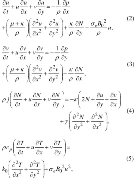
MHD Unsteady Flow and Heat Transfer of Micropolar

Fluid through Porous Channel with Expanding or

Contracting Walls

Y. Asia, A. Kashif and

A. Muhammad

†

Centre for Advanced Studies in Pure and Applied Mathematics, Bahauddin Zakariya University, Pakistan

†Corresponding Author Email: mashraf_mul@yahoo.com

(Received March 26, 2014; accepted September 6, 2015)

ABSTRACT

The unsteady laminar incompressible flow and heat transfer characteristics of an electrically conducting micropolar fluid in a porous channel with expanding or contracting walls is investigated. The relevant partial differential equations have been reduced to ordinary ones. The reduced system of ordinary differential equations (ODEs) has been solved numerically by lower-upper (LU) triangular factorization or Gaussian elimination and successive over relaxation (SOR) method. The effects of some physical parameters such as magnetic parameter, micropolar parameters, wall expansion ratio, permeability Reynolds number and Prandtl number on the velocity, microrotation, temperature and the shear and couple stresses are discussed.

Keywords: Magnetohydrodynamics (MHD); Expanding or contracting walls; Porous channel; Wall expansion ratio; Quasi-linearization.

1. INTRODUCTION

There are many fluids which are important from the industrial point of view, and display non-Newtonian behavior. Due to the complexity of such fluids, several models have been proposed but the micropolar model has been found to be the most appropriate one. It has been experimentally predicted that the fluids which could not be characterized by Newtonian relationships, indicated significant reduction in shear stress near a rigid body. The micropolar model has been successful in explaining such behaviors of the non-Newtonian fluids. Since its introduction, the micropolar fluid has been a hot area of research, and therefore many investigators have studied the related flow and heat transfer problems in different geometries. For example, natural convection heat transfer between two differentially heated concentric isothermal spheres utilizing micropolar fluid has been numerically investigated by Khoshab and Dehghan, (2011). Govardhan and Kishan (2011) studied the MHD effects on the unsteady boundary layer flow of an incompressible micropolar fluid over a stretching sheet when the sheet was stretched in its own plane. Ashmawy (2014) considered the problem of fully developed natural convective micropolar fluid flow in a vertical channel, under the slip boundary conditions for fluid velocity. The effect of the presence of a thin perfectly conductive baffle on the fully developed laminar mixed convection in a vertical channel containing

micropolar fluid was analyzed by Umavathi (2011).

There has been a growing interest of the research community in flows through porous channel with expanding or contracting walls. This is due to their significance in many biological and engineering models, including the transport of biological fluids through contracting or expanding vessels, the synchronous pulsation of porous diaphragms, the air circulation in the respiratory system, and the regression of the burning surface in solid rocket motors. Due to their extensive applications, many studies related to the internal flows in different geometries with contracting or expanding domains

have been carried out. Xin-Hue et al. (2011)

investigated the flow of a viscoelastic fluid in porous channels with expanding or contracting walls. Analytic solution of the problem was obtained by employing the homotopy analysis method (HAM) to the nolinear ODEs arising due to the introduction of similarity transformation. The study was further extended to the micropolar fluids

by Xin-Hue et al. (2010). Xinhui et al. 2012

considered the asymmetric viscoelastic fluid in a rectangular domain bounded by two porous moving channels with expanding or contracting walls.

(2)

micropolar fluid in a channel having permeable expanding or contracting walls, with an external magnetic field acting normally. A similarity transformation has been employed to construct a set of nonlinear coupled ordinary differential equations in the dimensionless form, which are numerically solved by employing an algorithm based on the Quasi-linearization and finite difference discretization. The ease in obtaining the numerical solution using the technique makes it superior than the shooting like approach used in our earlier investigations (for example, Ali et al. 2014)

2. PROBLEM

FORMULATION

We consider the flow and heat transfer characteristics of an unsteady, incompressible, viscous and electrically conducting micropolar fluid in a porous channel with expanding or contracting walls under the action of an external magnetic field. Compared to the imposed field, the induced magnetic field is assumed to be negligible. Further, the magnetic Reynolds number (defined as the ratio of the product of characteristic length and fluid velocity, to the magnetic diffusivity) is assumed to be small. For small magnetic Reynolds number, the magnetic field will tend to relax towards a purely diffusive state. Moreover, it is assumed that there is no applied polarization voltage which implies the absence of any electric field. Otherwise, the electrical current flowing in the fluid will give rise to an induced magnetic field which would exist if the fluid was an electrical insulator. But, in the present study, we have taken the fluid to be electrically conducting. The distance between the

porous walls is2a t

 

, which is much smaller than

the width and length of the channel. Both the channel walls have the same permeability and are expanding or contracting uniformly at a time-dependent rate a t

 

.

The geometry of the problem suggests that the Cartesian coordinate system may be chosen with the origin at the middle of the channel, as shown in the

Fig. 1. With u and v being the velocity

components in, respectively, the xand y directions,

the governing equations for the problem in the absence of body couples are:

Fig. 1. Physical model of the problem.

0,

u v

x y

 _ _

  (1)

2

2 2

0

2 2

1

,

e

u u u p

u v

t x y x

B

u u N

u y

x y





  

  

   

   

   

 

     

 _  _ _ 

 

  

(2)

2 2

1

,

v v v p

u v

t x y y

v v N

x

x y



  

 

 _  _  _{ } 

   

 

     

_ _  _



 

  

(3)

2 2

2

,

N N N u v

j u v N

t x y y x

N N

y x

 



 _  _  _{ }  _ _ 

_ _ _   _ _ 

   

  

 _  _

 

 

(4)

2 2

0 2 2 0 ,

p

e

T T T

c u v

t x y

T T

k B u

x y





 _  _  _

_ _ _ 

 

_ _ 

 

 

_ _ 

 

(5)

Here, , , T, c_pand 0 are, respectively, the

dynamic viscosity, density, temperature, specific heat at constant pressure, and thermal conductivity

of the fluid. Further, the symbolsj,  and 

denote the microinertia per unit mass, the spin gradient viscosity and the vortex viscosity of

micropolar fluids. Finally, e is the electrical

conductivity of the fluid, B0 is the strength of the

external magnetic field, and N is the component of

the microrotation normal to the xyplane.

It is important to mention that Eq. (1) is the continuity equation, Eqs. (2) and (3) correspond to the x- and y-components of the momentum equation (respectively), Eq. (4) is the microrotation equation, and finally Eq. (5) is the heat equation.

The micro-inertia density is the intensity of the inertial forces due to the micro particles of the fluid, whereas the microrotation is defined as the rotation of microscopic particles of a fluid, and is evaluated by taking the curl of the velocity field at microscopic level.

We also assume that there is strong concentration of microelements and the microelements close to the walls are unable to rotate. This assumption leads to the following boundary conditions for the problem:













 

1

2

, 0, , , , 0,

( , ) , , 0, , ,

, 0, ( , ) .

u x a v x a Aa N x a

T x a T u x a v x a Aa

N x a T x a T



      



    



  _



 (6)

Here

A

is the measure of the wall permeability,

and the dots denote the derivative w. r. t. the time

t

, whereas T1 and T2 (withT1T2) are the fixed

(3)

We introduce the following similarity transformations:

 

2 1 3 2 1 2 , , , , , , , . y

u a x F t

a t

v a F t N a x G t

T T T T                 _        _    _ (7)

It is to note that, with the above mentioned transformation, Eq. (1) is identically satisfied which means that the proposed velocity field is compatible with the continuity equation. It may, therefore, represent the possible fluid motion.

After eliminating the pressure term from the governing equations, we use Eq. (7) in the resulting equations, and arrive at:









1 2

2 2

0

(1 ) 3

0,

t

e

F G F F

F F FF a F

a B F            _ _                      _  (8)



 







2 1 2 3

2 t 0,

G G G F G FG

j a

G F a G

j       _ _   _        _         (9)





2

0

Pr F cpa _t 0.

k

  

       (10)

Here,  a a t( )



  is the wall expansion ratio,

Re Aa a



  is the permeability Reynolds number,

and

0

Pr cp

k



 is the Prandtl number.

The boundary conditions acquire the form:

1; Re, 0, 0, 1,

1; Re, 0, 0, 0.

F F G

            _{ } 

     _ (11)

Finally, we set Re

F f ,

Re

G

g , and consider the

case following Majdalani and Zhou, 2003 when



is a constant, ff( )

, g g ( ) and  

 

, which leads to _t0, g_t0 and ft0.

Thus we have the following equations













1 1

1 3

Re 0,

C f C g f f

f f ff Mf

   

   

 

   

    (12)







 



3 2

2 1

3

Re 2 0,

C g C g g

C f g f g C g f

 

  

 

  

    (13)





Pr Ref 0,

 

     (14)

where 2 2 0 e a B M  

 is magnetic parameter,

1

C 



 is vortex viscosity parameter, 2 ₂

j C

a

 is

microinertia density parameter and C3 ₂

a

 

 is

spin gradient viscosity parameter.

The boundary conditions (11) are reduced as

1;f 1,f_ 0,g 0, 1

       and

1;f 1,f_ 0,g 0, 0.

     (15)

3. NUMERICAL

SOLUTION

We use quasi-linearization to construct three

sequences of vectors

 

f k ,

 

g k and

 

 k , which converge to the numerical solutions of Eqs. (12), (13) and (14) respectively. To construct

 

 

k

f we linearize Eq. (12), by retaining only the

first order terms, as follows:

We set

























1 1 ( ) ( ) ( ) ( ) ( )

( 1) ( ) ( 1) ( )

( ) ( )

( 1) ( ) ( 1) ( )

( )

( , , , , ) 1

(3 ) Re ,

( k , k , k, k, k )

k k k k

k k

k k k k

k

f f f f f C f

f f f f ff C g Mf

f f f f f

f f f f

f f

f f f f

f f                                                             





( )

( 1) ( )

( ) 0,

k k k k f f f           (16) which yields









   





     

( 1) ( ) ( 1)

1

( 1)

1 ( ) ( 1)

( ) ( ) ( )

1

1 Re

(3 Re )

Re Re

k k k

k k

k k k k

k k

k k k

C f f f

f M f

f f f f

f f C g f f

                              (17)

Now Eq. (17) gives a system of linear differential

equations, with _fk

being the numerical solution

vector of the th

k equation. To solve the linear

(4)

sequence

 

f k , generated by the following linear system:

(k 1)

Bf  C (18)

with BBn n

 

f( )k andCCn1

 

f( )k , where n

is the number of grid points. On the other hand,

Eqs. (13) and (14) are linear in gand 

respectively, and therefore, in order to generate the

sequences

 

g k and

 

 k , we write:

 



 



 





   





1 1 ( 1)

3 2

1 ( 1) 1

1 1

( 1) ( 1)

2

3

2

Re 0,

k k k

k k

C g C g g

C f g

C f g f g

 



 

 

  

 

  

 

  (19)

 ₁



 ₁



 1

Pr Re k 0,

k k

f

 

        (20)

Importantly f(k1) is considered to be known in

the above equations and its derivatives are approximated by the respective central differences approximations.

It is important to note that the coefficient

matrixB in Eq. (18) will be pentadiagonal and

not diagonally dominant, and hence the iterative method like Successive over relaxation (SOR) may fail or work very poorly. Therefore, some direct method like Lower-Upper (LU) triangular factorization or Gaussian elimination with full pivoting (to ensure stability) may be employed. On the other hand, Eqs. (19) and (20) will give rise to the diagonally dominant algebraic system when discretized using the central differences, which allows us to use the SOR method. Lastly, we may also improve the order of accuracy of the solution by using polynomial extrapolation scheme.

4. RESULTS

AND

DISCUSSION

In this section, we will interpret the graphical and tabular presentation of our results. The physical quantities of our interest are the shear stresses, the couple stresses and the heat transfer rates at the channel walls which are, respectively, proportional to f

   

1 ,g 1 and 

 

1 . Because of the symmetry of the problem, the results are given only at the lower wall. The physical parameters of the problem are the Reynolds number Re, the magnetic parameter

,

M the Prandtl number Pr, the wall expansion

ratio



and the micropolar parameters C C1, 2

andC3. We shall study the effect of the

parameters onf

   

1 ,g 1 and 

 

1 , as well

as, on the velocity profilesf

   

 ,f , the

microrotation profileg

 

 , and the heat

profile 

 

. It is to note that 0 or 0 according to the case when the channel walls are

contracting or expanding, whereas Re0 for

suction.

The values of micropolar parameters C C₁, ₂&C₃

are chosen arbitrarily (given in Table 1), whereas the first case corresponds to the Newtonian fluid.

Table 1 Values of micropolar parameters used in the present study

Cases C₁ C₂ C₃

1 2 3 4 5

0 2 4 6 8

0 0.4 0.8 1.2 1.6

0 0.3 0.4 0.5 0.6

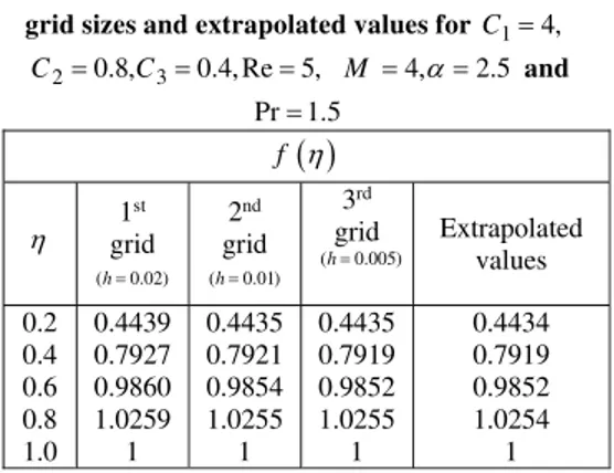
Table 2 shows the convergence of our numerical results as the step-size decreases, which gives us confidence on our computational procedure.

Table 2 Dimensionless velocity f

 

 on three grid sizes and extrapolated values for C₁4,

2 0.8, 3 0.4, Re 5,

C  C   M 4,2.5 and

Pr1.5

 

f 

 1

st

grid

(h0.02)

2nd

grid

(h0.01)

3rd

grid

(h0.005)

Extrapolated values

0.2 0.4 0.6 0.8 1.0

0.4439 0.7927 0.9860 1.0259

1

0.4435 0.7921 0.9854 1.0255

1

0.4435 0.7919 0.9852 1.0255

1

0.4434 0.7919 0.9852 1.0254

1

Table 3 shows that the effect of micropolar structure of the fluid is to reduce the shear stresses while increasing the couple stresses and the heat transfer rates at the channel walls, whether the walls are expanding or contracting. It is further noted that, compared with the shear and couple stresses, the effect of the micropolar parameters on the heat transfer rate is not much pronounced. It is perhaps due the reason that the micropolar parameters do not appear in the heat equation (please see Eq. (14)), and therefore do not influence the heat transfer rate directly.

Table 3 Effect of the micropolar parameters on

   

1 , 1

f  g  and  

 

1 for Re1,M 4

and Pr1.5

Cases

_{ }

 1.5

1

 

f g 

 

1  

 

1 1

2 3 4 5

4.8919 3.3166 2.9428 2.7788 2.6871

0 4.7287 6.4612 7.4153 8.0260

(5)

Cases

_{ }

1.5

1

 

f f

 

1 f

 

1

1 2 3 4 5

2.6648 2.3005 2.0183 1.8593 1.7587

Table 4 shows that the shear stress increases with the Reynolds number while slightly decreasing the heat transfer rate, for the case of contracting channel walls. However, the trend is reversed for the expanding walls. On the other hand, a remarkable rise in the couple stress is noted whether the walls are approaching or receding.

Table 4 Effect of the Reynolds number Reon

   

1 , 1

f  g  and  

 

1 for 1 4, 2 0.8,

C  C  C30.4,M 4 and Pr1.5.

Re

_{ }

 1.5

1  

f g 

 

1  

 

1 3.0

3.5 4.0 4.5 5.0

2.9879 3.0032 3.0199 3.0378 3.0567

8.4576 8.9771 9.4985 10.0192 10.5374

-1.5590 -1.5587 -1.5585 -1.5582 -1.5580

Re

_{ }

 1.5

1  

f g 

 

1  

 

1 3.0

3.5 4.0 4.5 5.0

1.6564 1.5667 1.4844 1.4125 1.3527

10.1184 11.7264 13.5062 15.4296 17.4634

-0.4383 -0.4386 -0.4388 -0.4389 -0.4390

It is obvious from the Table 5 that the role of the external magnetic field is to enhance both the shear and couple stresses while lowering the heat transfer rate, for both the cases of .

Table 5 Effect of the magnetic parameter M on

   

1 , 1

f  g  and  

 

1 for 1 4, 2 0.8,

C  C  C30.4, Re1 and Pr1.5

M

1.5

 

 

1



f g 

 

1  

 

1

0 25 50 75 100

2.7832 3.6593 4.3340 4.8900 5.3675

6.3829 6.7894 7.0627 7.2619 7.4151

-1.5619 -1.5511 -1.5437 -1.5382 -1.5339

M 1.5



 

1



f g 

 

1  

 

1

0 25 50 75 100

1.8141 2.8971 3.6818 4.3067 4.8321

5.4674 6.0599 6.4369 6.7037 6.9053

-0.4385 -0.4300 -0.4247 -0.4211 -0.4183

Table 6 predicts that the wall expansion ratio increases the shear and couple stresses as well as the heat transfer rate, when the walls are contracting. Again, a completely opposite trend is noted for the expanding walls.

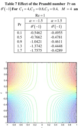
It is clear from the Table 7 that the Prandtl number enhances the heat transfer rate only in case of contracting walls. It does not affect the other two physical quantities, due to the one way coupling of the governing equations (please see Eqs. (12)-(14) ).

Physical model of the problem is shown in the Fig. 1, whereas the streamlines for the present problem are shown in the Fig. 2.

Table 6 Effect of the wall expansion ratio  on

   

1 , 1

f  g  , 

 

1 for C₁4,

2 0.8, 3 0.4, 4, Pr 1.5

C  C  M   and Re1

 f

 

1 g 

 

1  

 

1 -2.5

-1.5 0.0 1.5 2.5

3.1683 2.9428 2.5485 2.0183 1.4886

6.6371 6.4612 6.1076 5.5850 5.0734

-2.1421 -1.5599 -0.8755 -0.4368 -0.2608

Table 7 Effect of the Prandtl number Pron

 

1

  For C₁4,C₂0.8,C₃0.4, M 4 and

Re1

Pr

1.5

  1.5

 

1

   

 

1 0.1

0.5 0.9 1.3 1.7

-0.5462 -0.7662 -1.0421 -1.3742 -1.7575

-0.4955 -0.4781 -0.4611 -0.4448 -0.4289

r

z

-1 -0.8 -0.6 -0.4 -0.2 0 0.2 0.4 0.6 0.8 1 -1

-0.8 -0.6 -0.4 -0.2 0 0.2 0.4 0.6 0.8 1

Fig. 2. Contours of stream function for

1 4, 2 0.8, 3 0.4, Re 5, Pr 1.5,

C  C  C   

2.5,M 4

  .

It is to mention that the position of viscous layer (the point  0 for whichf

 

 0) lies in the

middle of the channel, that is, in the planez0,

(6)

However, it may shift towards either of the walls for the asymmetrical case, which may be a topic of a subsequent study. Moreover, the normal velocity

takes its dimensionless value 1 at the lower wall,

and acquires its maximum value 1 at the upper one,

with a point of inflection lying at 0(due to the

symmetry of the problem) where it changes its concavity.

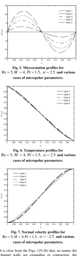
Figures (3-10) reflect the effect of the micropolar parameters on the velocity, microrotation and heat

profiles. It is noted that, for both the cases of ,

the micropolar parameters increase the magnitude of the normal velocity and the microrotation across the whole computational domain. The streamwise velocity is, however, raised only in the middle of the channel. Again, the micropolar parameters are not much influential for the thermal distribution.

For the case of expanding walls, the effect of the Reynolds number is similar to that of micropolar parameters (please see Figs. (11-18)). however, for the other case, we note two points: the Reynolds number is not much influential; and the way it affects the streamwise velocity and the microrotation, is changed.

-1 -0.8 -0.6 -0.4 -0.2 0 0.2 0.4 0.6 0.8 1 -1.5

-1 -0.5 0 0.5 1 1.5



f (



)

Case 1 Case 2 Case 3 Case 4 Case 5

Fig. 3. Normal velocity profiles for

Re



5,

M



4,

Pr



1.5,





2.5

and various cases of micropolar parameters.

-1 -0.8 -0.6 -0.4 -0.2 0 0.2 0.4 0.6 0.8 1

-1 -0.5 0 0.5 1 1.5 2 2.5 3 3.5



f'

(

)

Fig. 4. Streamwise velocity profiles for

Re5,M 4, Pr1.5,2.5 and various cases of micropolar parameters.

-1 -0.8 -0.6 -0.4 -0.2 0 0.2 0.4 0.6 0.8 1

-15 -10 -5 0 5 10 15



g (



)

Fig. 5. Microrotation profiles for

Re



5,

M



4, Pr



1.5,

 

2.5

-1 -0.8 -0.6 -0.4 -0.2 0 0.2 0.4 0.6 0.8 1 0

0.1 0.2 0.3 0.4 0.5 0.6 0.7 0.8 0.9 1





( 

)

Fig. 6. Temperature profiles for

Re



5,

M



4, Pr



1.5,

 

2.5

-1 -0.8 -0.6 -0.4 -0.2 0 0.2 0.4 0.6 0.8 1



f (



)

Fig. 7. Normal velocity profiles for

Re5,M4, Pr1.5,

  

2.5

(7)

results in increasing the shear stress at the wall but also causes greater spinning of the micro fluid particles hence, increases the couple stress as well (evident from Table 5).

-1 -0.8 -0.6 -0.4 -0.2 0 0.2 0.4 0.6 0.8 1

-0.2 0 0.2 0.4 0.6 0.8 1 1.2 1.4 1.6



f'

(



)

Fig. 8. Streamwise velocity profiles for

Re



5,

M



4,

Pr



1.5,



 

2.5

and various cases of micropolar parameters.

-1 -0.8 -0.6 -0.4 -0.2 0 0.2 0.4 0.6 0.8 1

-0.8 -0.6 -0.4 -0.2 0 0.2 0.4 0.6



g (



)

Fig. 9. Microrotation profiles for

Re



5,

M



4, Pr



1.5,

  

2.5

-1 -0.8 -0.6 -0.4 -0.2 0 0.2 0.4 0.6 0.8 1

0 0.1 0.2 0.3 0.4 0.5 0.6 0.7 0.8 0.9 1





(



)

Fig. 10. Temperature profiles for

Re



5,

M



4, Pr



1.5,

  

2.5

and various cases of micropolar parameters.

-1 -0.8 -0.6 -0.4 -0.2 0 0.2 0.4 0.6 0.8 1 -1.5

-1 -0.5 0 0.5 1 1.5



f (



)

Re = 1 Re = 5 Re = 9 Re = 13 Re = 17

Fig. 11. Normal velocity profiles for 1 4, 2 0.8, 3 0.4,

C  C  C  M 4,

Pr1.5,2.5 and various

Re

.

-1 -0.8 -0.6 -0.4 -0.2 0 0.2 0.4 0.6 0.8 1 -1

-0.5 0 0.5 1 1.5 2 2.5 3



f'

(

)

Re = 1 Re = 5 Re = 9 Re = 13 Re = 17

Fig. 12. Streamwise velocity profiles for 1 4, 2 0.8,

C  C  C₃0.4,M 4, Pr1.5,2.5 and variousRe.

-1 -0.8 -0.6 -0.4 -0.2 0 0.2 0.4 0.6 0.8 1

-15 -10 -5 0 5 10 15



g (



)

Re = 1 Re = 5 Re = 9 Re = 13 Re = 17

Fig. 13. Microrotation profiles for 1 4, 2 0.8, 3 0.4,

C  C  C  M 4,

Pr1.5,2.5 and various Re.

-1 -0.8 -0.6 -0.4 -0.2 0 0.2 0.4 0.6 0.8 1 0

0.1 0.2 0.3 0.4 0.5 0.6 0.7 0.8 0.9 1





(



)

Re = 1 Re = 5 Re = 9 Re = 13 Re = 17

Fig. 14. Temperature profiles for 1 4, 2 0.8, 3 0.4,

C  C  C  M 4,

(8)

-1 -0.8 -0.6 -0.4 -0.2 0 0.2 0.4 0.6 0.8 1 -1

-0.8 -0.6 -0.4 -0.2 0 0.2 0.4 0.6 0.8 1



f (



)

Re = 1 Re = 5 Re = 9 Re = 13 Re = 17

Fig. 15. Normal velocity profiles for 1 4, 2 0.8,

C  C 

C

₃



0.4,

4, Pr 1.5, 2.5

M     and various Re.

-1 -0.8 -0.6 -0.4 -0.2 0 0.2 0.4 0.6 0.8 1 -0.2

0 0.2 0.4 0.6 0.8 1 1.2 1.4 1.6



f'

(



)

Re = 1 Re = 5 Re = 9 Re = 13 Re = 17

C  C  C₃0.4,M 4, Pr1.5, 2.5 and various Re.

-1 -0.8 -0.6 -0.4 -0.2 0 0.2 0.4 0.6 0.8 1 -0.5

-0.4 -0.3 -0.2 -0.1 0 0.1 0.2 0.3 0.4 0.5



g (



)

Re = 1 Re = 5 Re = 9 Re = 13 Re = 17

Fig. 17. Microrotation profiles for 1 4, 2 0.8,

-1 -0.8 -0.6 -0.4 -0.2 0 0.2 0.4 0.6 0.8 1 0

0.1 0.2 0.3 0.4 0.5 0.6 0.7 0.8 0.9 1





( 

)

Re = 1 Re = 5 Re = 9 Re = 13 Re = 17

Fig. 18. Temperature profiles for 1 4, 2 0.8,

-1 -0.8 -0.6 -0.4 -0.2 0 0.2 0.4 0.6 0.8 1 -1

-0.8 -0.6 -0.4 -0.2 0 0.2 0.4 0.6 0.8 1



f (



)

M = 0 M = 25 M = 50 M = 75 M = 100

C  C  C₃0.4, Pr1.5,

Re2,2.5 and various M.

-1 -0.8 -0.6 -0.4 -0.2 0 0.2 0.4 0.6 0.8 1 -0.5

0 0.5 1 1.5 2



f'

(

)

M = 0 M = 25 M = 50 M = 75 M = 100

C  C  C₃0.4, Pr1.5,

Re



2,





2.5

and various M .

-1 -0.8 -0.6 -0.4 -0.2 0 0.2 0.4 0.6 0.8 1

-3 -2 -1 0 1 2 3



g (



)

M = 0 M = 25 M = 50 M = 75 M = 100

C  C  C₃0.4, Pr1.5,

Re2,2.5 and various M .

-1 -0.8 -0.6 -0.4 -0.2 0 0.2 0.4 0.6 0.8 1 0

0.1 0.2 0.3 0.4 0.5 0.6 0.7 0.8 0.9 1





(



)

M = 0 M = 25 M = 50 M = 75 M = 100

C  C  C₃0.4, Pr1.5,

(9)

-1 -0.8 -0.6 -0.4 -0.2 0 0.2 0.4 0.6 0.8 1 -1

-0.8 -0.6 -0.4 -0.2 0 0.2 0.4 0.6 0.8 1



f (



)

M = 0 M = 25 M = 50 M = 75 M = 100

C  C  C₃0.4, Pr1.5,

Re2, 2.5 and various M.

-1 -0.8 -0.6 -0.4 -0.2 0 0.2 0.4 0.6 0.8 1 -0.2

0 0.2 0.4 0.6 0.8 1 1.2 1.4 1.6



f'

(

)

M = 0 M = 25 M = 50 M = 75 M = 100

C  C  C₃0.4, Pr1.5,

Re2, 2.5 and various M .

-1 -0.8 -0.6 -0.4 -0.2 0 0.2 0.4 0.6 0.8 1 -0.5

-0.4 -0.3 -0.2 -0.1 0 0.1 0.2 0.3 0.4 0.5



g (



)

M = 0 M = 25 M = 50 M = 75 M = 100

C  C  C₃0.4, Pr1.5,

Re2, 2.5and various M .

-1 -0.8 -0.6 -0.4 -0.2 0 0.2 0.4 0.6 0.8 1 0

0.1 0.2 0.3 0.4 0.5 0.6 0.7 0.8 0.9 1





(



)

M = 0 M = 25 M = 50 M = 75 M = 100

C  C  C₃0.4, Pr1.5,

Re2, 2.5 and various M.

As  varies from negative to positive, we note

the rise in the magnitudes of the normal velocity and the microrotaion across the whole domain. The temperature profile, however, tends to become an almost linear function of the

dimensionless spatial variable  (please see

Figs. (27-30)).

-1 -0.8 -0.6 -0.4 -0.2 0 0.2 0.4 0.6 0.8 1 -1

-0.8 -0.6 -0.4 -0.2 0 0.2 0.4 0.6 0.8 1



f (



)

 = -2.5

 = -1.5

 = 0.0

 = 1.5

 = 2.5

C  C  C₃0.4,M 4,

Re2, Pr1.5 and various



.

Fig. 28. Streamwise velocity profiles for C₁4,

2 0.8, 3 0.4, 4,

C  C  M  Re2, Pr1.5 and

various



.

-1 -0.8 -0.6 -0.4 -0.2 0 0.2 0.4 0.6 0.8 1

-3 -2 -1 0 1 2 3



g (



)

 = -2.5

 = -1.5

 = 0.0

 = 1.5

 = 2.5

Fig. 29. Microrotation profiles forC₁4,C₂0.8,

3 0.4, 4,

(10)

-1 -0.8 -0.6 -0.4 -0.2 0 0.2 0.4 0.6 0.8 1 0

0.1 0.2 0.3 0.4 0.5 0.6 0.7 0.8 0.9 1





( 

)

 = -2.5  = -1.5  = 0.0  = 1.5  = 2.5

C  C  C₃0.4,M 4,

Re2, Pr1.5 and various



.

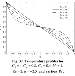
Figures (31-32) show that, in the case of contracting walls, the Prandtl number tends to lower the thermal distribution in the lower half of the channel whereas an opposite effect is noted in the upper half. The trend is however reversed for the case of expanding walls.

Compared with the work of Aski et al. 2014, we

have noticed a qualitative change in the way in which the micropolar parameters and the Reynolds number affect the streamwise velocity profiles in case of expanding walls. Both the parameters tend to lower the velocity distribution near both the walls, predicting a negative velocity component in these regions. Thus, the parabolic nature of the profile for the Newtonian fluid at low Reynolds number is changed. No such change was noticed in

the work of Aski et al. 2014, where the channels

were stationary. We therefore conclude that this particular influence of the micropolar parameters and the Reynolds number is due to the expanding channel walls. Moreover, we notice a non uniform way in which the Reynolds number affects the microrotation profiles for the case of approaching walls. It decreases the magnitude of the microrotation everywhere except for the small regions near the two walls where the trend is opposite, which is again contrary to the results reported by Aski et al. 2014.

-1 -0.8 -0.6 -0.4 -0.2 0 0.2 0.4 0.6 0.8 1

0 0.1 0.2 0.3 0.4 0.5 0.6 0.7 0.8 0.9 1





( 

)

Pr = 0.1 Pr = 0.5 Pr = 0.9 Pr = 1.3 Pr = 1.7

Fig. 31. Temperature profiles forC₁4,C₂0.8, C₃0.4,M 4,

Re2,2.5 and various Pr.

-1 -0.8 -0.6 -0.4 -0.2 0 0.2 0.4 0.6 0.8 1

0 0.1 0.2 0.3 0.4 0.5 0.6 0.7 0.8 0.9 1





(



)

Pr = 0.1 Pr = 0.5 Pr = 0.9 Pr = 1.3 Pr = 1.7

C  C  C₃0.4,M 4, Re2, 2.5 and various Pr.

5. CONCLUSUONS

The characteristics of laminar, incompressible, viscous and unsteady flow of an electrically conducting micropolar fluid in a porous channel with expanding or contracting walls under the action of an applied magnetic field are explored numerically.

It has been observed that the micropolar structure of the fluid is responsible for reducing the shear stress while increasing the couple stress and the heat transfer rate at the channel walls, whether the walls are expanding or contracting. The shear stress increases with the Reynolds number while slightly decreasing the heat transfer rate, only for the case of contracting channel walls. The external magnetic field always enhances both the shear and couple stresses while lowering the heat transfer rate. The wall expansion ratio increases or decreases the three physical quantities according to the case of contracting or expanding walls, whereas the Prandtl number enhances the heat transfer rate only in case of contracting walls.

The micropolar parameters increase the magnitudes of the normal velocity and the microrotation across the channel, for the both wall conditions. For approaching walls, the Reynolds number decreases the magnitude of the microrotation everywhere except for the small regions near the two walls where the trend is opposite. No matter the channel walls are expanding or contracting, the magnetic field reduces the normal velocity and the microrotation. In case of expanding walls, the micropolar parameters and the Reynolds number tend to lower the velocity distribution near both the channel walls, predicting a negative velocity component in these regions. For contracting walls, the Prandtl number tends to lower the thermal distribution in the lower half of the channel whereas an opposite effect is noted in the upper half. The trend is however reversed for the case of expanding walls.

ACKNOWLEDGEMENTS

(11)

Education Commission of Pakistan for the financial support to carry out this research. The authors are also grateful to the learned reviewers for their comments to improve the quality of this paper.

REFERENCES

Ali, K. and M. Ashraf (2014). Numerical simulation of the micropolar fluid flow and heat transfer in a channel with a shrinking and a stationary wall.

Journal of Theoretical and Applied Mechanics

52, 557-569.

Ali, K., F. M. Iqbal, Z. M. Akbar and M. Ashraf (2014). Numerical simulation of unsteady water-based nanofluid flow and heat transfer between two orthogonally moving porous coaxial disks.

Journal of Theoretical and Applied Mechanics

52, 1033-1046.

Ali, K., M. Ashraf, and N. Jameel (2014). Numerical simulation of magnetohydro dynamic micropolar fluid flow and heat transfer in a

channel with shrinking walls. Canadian Journal

of Physics 92(9), 987-996.

Ali, K., Z. M. Akbar, F. M. Iqbal and M. Ashraf (2014). Numerical simulation of heat and mass transfer in unsteady nanofluid between two

orthogonally moving porous coaxial disks. AIP

Advances. 4.

Ashmawy, E. A. (2014). Fully developed natural convective micropolar fluid flow in a vertical

channel with slip. Journal of the Egyptian

Mathematical Society.

Govardhan, K. and N. Kishan (2011). Unsteady MHD boundary layer flow of an incompressible

micropolar fluid over a stretching sheet. Journal

of Applied Fluid Mechanic. 5(3), 23-28.

Khoshab, M. and A. A. Dehghan (2011). Numerical simulation of buoyancy-induced micropolar fluid flow between two concentric isothermal spheres.

Journal of Applied Fluid Mechanic 4(2), 51-59.

Majdalani, J. and C. Zhou (2003). Moderate-to-large injection and suction driven channel flows

with expanding or contracting walls. Zeitschrift

fur Angewandte Mathematik and Mechanik

83(3), 181-196.

Umavathi, J. C. (2011). Mixed convection of micropolar fluid in a vertical double-passage

channel. International Journal of Engineering,

Science and Technology 3(8), 197-209.

Xin-Hue, SI. , Z. Lian-Cun, Z. Xin-Xin and Y. Chao (2010). Analytic solution to the micropolar fluid flow through a semi-porous channel with an

expanding or contracting wall. Applied

Mathematics and Mechanics –English Edition

31(9) 1073–1080.

Xin-Hue, SI., Z. Lian-Cun, Z. Xin-Xin, SI. Xin-Yi and Y. Jian-Hong (2011). Flow of a viscoelastic fluid through a porous channel with expanding or

contracting walls. Chin. Phys. Lett. 28(4),

044702.

Xinhui, S., Z. Liancun, Z. Xinxin, S. Xinyi, and L. Min (2012). Asymmetric viscoelastic flow through a porous channel with expanding or contracting walls: a model for transport of

biological fluids through vessels. Computer

(12)