An information theoretic approach for
pri-vacy metrics
Michele Bezzi
SAP Labs.F-06560, Mougins, France
E-mail:[email protected]
Abstract. Organizations often need to release microdata without revealing sensitive information. To this scope, data are anonymized and, to assess the quality of the process, various privacy metrics have been proposed, such as k-anonymity,ℓ-diversity, andt-closeness. These metrics are able to capture different aspects of the disclosure risk, imposing minimal requirements on the association of an individual with the sensitive attributes. If we want to combine them in a optimization problem, we need a common framework able to express all these privacy conditions. Previous studies proposed the notion of mutual information to measure the different kinds of disclosure risks and the utility, but, since mutual information is an average quantity, it is not able to completely express these conditions on single records. We introduce here the notion of one-symbol information (i.e., the contribution to mutual information by a single record) that allows to express and compare the disclosure risk metrics. In addition, we obtain a relation between the risk valuestandℓ, which can be used for parameter setting. We also show, by numerical experiments, howℓ-diversity andt-closeness can be represented in terms of two different, but equally acceptable, conditions on the information gain.
Keywords. Database Applications-Statistical databases; Systems and Information Theory; Anonymiza-tion
1
Introduction
Governmental agencies and corporates hold a huge amount of data containing information on individual people or companies (micro data). They have often to release part of these data for research purposes, data analysis or application testing. However, these data con-tain sensitive information and organizations are hesitant to publish them. To reduce the risk, data publishers use masking techniques (anonymization) for limiting disclosure risk in releasing sensitive datasets. In many cases, the data publisher does not know in advance the data mining tasks performed by the recipient, or even it does not know who the re-cipients are (so calledprivacy preserving data publishing[18]). Therefore, the data publisher tasks are basically to anonymize (under some privacy constraints) and to release the data.
0Some parts of this paper has been presented at the International Conference on Privacy in Statistical
In other scenarios, the data publishers may know the data mining activities in advance (privacy preserving data mining scenario), therefore they can customize the anonymiza-tion to preserve some statistical properties. In this paper we will mainly focus on the first scenario, privacy preserving data publishing, which is relevant in many real use cases, such as creating test data for application testing, outsourcing the development of new mining algorithms [2], and it is also pushed by regulatory frameworks [9].
Typically, data are contained in tables, and the attributes (columns) in the original table can be categorized, from disclosure perspective, in the following types:
• Identifiers. Attributes that explicitly identify individuals. E.g., Social Security Num-ber, passport numNum-ber, complete name.
• Quasi-identifiers (QIs) or key attributes[10]. Attributes that in combination can be used to identify an individual E.g., Postal code, age, gender, etc ... .
• Sensitive attributes. Attributes that contain sensitive information about an individual or business, e.g., salary, diseases, political views, etc ...
Various anonymization methods can be applied to obfuscate the sensitive information, they include: generalizing the data, i.e., recoding variables into broader classes (e.g., re-leasing only the first two digits of the zip code) or rounding numerical data, suppressing part of or entire records, randomly swapping some attributes in the original data records, permutations or perturbative masking, i.e., adding random noise to numerical data val-ues. These anonymization methods increase protection, lowering the disclosure risk, but, clearly, they also decrease the quality of the data and hence its utility [14]. There are two types of disclosure: identity disclosure, and attribute disclosure. Identity disclosure oc-curs when the identity of an individual is associated with a record containing confidential information in the released dataset. Attribute disclosure occurs when an attribute value may be associated with an individual (without necessarily being able to link to a specific record). Anonymizing the original data, we want to prevent both kinds of disclosures. In the anonymization process Identifiers are suppressed (or replaced with random values), but this is not sufficient, since combining the quasi-identifiers values with some external source information (e.g., a public register) an attacker could still be able to re-identify part of the records in the dataset. To reduce the risk some of the masking techniques described above are applied on the quasi-identifiers. To assess the quality of the anonymization pro-cess, there is the need to measure the disclosure risk in the anonymized dataset and its utility. Typically, disclosure risk metrics are set to define the privacy constraints, and then we look for the masking mechanisms that maximize the utility. Both disclosure risk and utility metrics are hard to define in general, because they may depend on context variables, e.g., data usage, level of knowledge of the attacker, amount of data released, etc..., and many possible definitions have been proposed so far.
We focus here on disclosure risk measures. Various models have been proposed to capture different aspects of the privacy risk (see [18] for a review). From the data publisher point of view, it would be desirable to have these privacy models expressed in terms of semantically “similar” measures, so he could be able to compare their impact and optimize the trade off between the different privacy risks.
wide range of well established information theory tools to risk optimization (e.g., privacy-distortion trade off problem [24]). Note that, mutual information (or, similarly, information loss) has been also proposed as utility measure [11]. Although, we will use this definition in our simulations (see Sect. 4), the main focus of our paper is investigating how we can compare the different privacy metrics among them, independently on the utility metrics used.
In this paper, we extend the information theoretic formulation of disclosure risk mea-sures. In particular, existing privacy metrics (k-anonymity,ℓ-diversity and t-closeness met-rics [25, 22, 20]) define minimal requirements for each entry (or QI group) in the dataset, but because mutual information is an average quantity, it is not able to completely express these conditions on single entries. In fact, as pointed out in [21], privacy is an individual concept and should be measured separately for each individual, accordingly average measures, as mutual information, are not able to fully capture privacy risk.
Thus, we introduce here two types of one-symbol information (i.e., the contribution to mutual information by a single record), and define the disclosure risk metrics in terms of information theory (see Sect. 3). By introducing one-symbol information we are able to express and compare different risk concepts, such ask-anonymity, ℓ-diversity and t -closeness, using the same units. In addition, we obtain a set of constraints on the mutual and one-symbol information for satisfyingℓ-diversity and t-closeness. We also derive a relation between the risk parameterstandℓ, which allows to assesstin terms of the more intuitiveℓvalue.
We present a simple example, to point out that in presence of a constant average risk, the records at risk may depend on the information metric used (Sect. 3.1). In Sect. 4, we test our framework, using a census dataset, to show the relevant differences between risk estimation based on average measures, as mutual information, and record specific metrics, as one-symbol information. We also show how focusing on the information contribution of a single record or group, we can minimize the information loss during anonymization. Lastly, we discuss our results and introduce some directions for future work.
In summary, this paper does not provide a unique answer to what disclosure risk is, but it gives the necessary theoretical ground for expressing and comparing different risk mea-sures, and provides some useful relations for setting risk parameters.
Before entering in details about the proposed model, in the following sections we will introduce some background on disclosure risk metrics (Sect. 2.1) and information theory (Sect. 2.2).
2
Preliminaries
2.1
Privacy Metrics
Let us consider a dataset containing identifiers, quasi-identifiers (QIs),X, and sensitive at-tributes,W (for example as in Table 2). We create an anonymized version of such data, re-moving identifiers, and anonymizing quasi-identifiers (X˜), for example generalizing them in classes (see Table 3).
To estimate the disclosure risk in the anonymized data, various metrics have been pro-posed so far.
probability1/kto re-identify a record, but it does not necessarily protect against attribute disclosure. In fact, a QI group (with minimal size ofkrecords) could also have the same confidential attribute, so even if the attacker is not able to re-identify the record, he can discover the sensitive information.
To capture this kind of riskℓ-diversity was introduced [22].ℓ-diversity condition requires that foreverycombination of key attributes there should be at least ℓ“well represented” values for each confidential attribute. In the original paper, a number of definitions of “well represented” were proposed. Because we are interested here in providing an information-theoretic framework, the more relevant for us is in terms of entropy, i.e.,
H(W|x)˜ ≡ − X
w∈W
p(w|˜x) log2p(w|x)˜ ≥log2ℓ
for every QI groupx˜, and with ℓ ≥ 1. For example, if each QI group have n equally distributed values for the sensitive attributes, the entire dataset will ben-diverse. Note that ifℓ-diversity condition holds, also thek-anonymity condition (withk ≤ ℓ) automatically holds, since there should be at leastℓrecords for each group of QIs.
Although,ℓ-diversity condition prevents the possible attacker to infer exactly the sensitive attributes, he may still learn a considerable amount of probabilistic information. In partic-ular if the distribution of confidential attributes within a QI group is very dissimilar from the distribution over the whole set, an attacker may increase his knowledge on sensitive attributes (skewness attack, see [20] for details). t-closeness estimates this risk by computing the distance between the distribution of confidential attributes within the QI group and in the entire dataset. The authors in [20] proposed two ways to measure the distance, one of them has a straightforward relationship with mutual information (see Eq. 7 below), as we discuss in the next section.
Another notion for assessing the privacy risk is differential privacy [15]. The basic idea is that the removal, addition or replacement of a single personal information (a record) in the original database should not significantly impact the outcome of any statistical analy-sis. This privacy model requires that the data publisher knows in advance the exact set of queries/analysis that need to be performed on the released data. However, this does not fit the requirements of theprivacy preserving data publishingscenario we are addressing in this paper. We will discuss possible extension to include differential privacy in our framework in the last section.
These measures provide a quantitative assessment of the different risks associated to data release, but they have also major limitations. First, they impose strong constraints on the anonymization, resulting in a large utility loss; second, it is often hard to find a computa-tional procedure to achieve a pre-defined level of risk; third, since they capture different features of disclosure risks, they are difficult to compare and optimize at the same time. To address the last point, we propose in the next sections a common framework, one-symbol information, for expressing these three risk measures. We will discuss the first two issues, in the last Section.
2.2
Information theory
Definition Positive Chain rule Chain rule Average
definite X Y MI
I1 Yes Yes No Yes
I2 No Yes Yes Yes
I3 No Yes No Yes
I4 Yes Yes Yes/No No
Table 1: Main properties of the four definitions of one-symbol information. I1andI2are
discussed in the main text,I3(x, Y)≡Py∈Y p(y|x)[H(X)−H(X|y)][8] is a definition based on weighted average of reduction of uncertainty,I4(x, Y)≡I({x,x¯};Y)[3] is the mutual
information betweenY and a set composed by two elements:xand its complement inX: ¯
x≡X\x. For more details, see [5].
andp(x|y)the corresponding joint and conditional probability functions. Following Shan-non [26], we can define the mutual informationI(X;Y)as:
I(X;Y) = X
x∈X,y∈Y
p(x, y) log2
p(x, y)
p(x)p(y)
= X
x∈X,y∈Y
p(y)p(x|y) log2
p(x|y)
p(x)
, (1)
(with conditional probability p(x|y) = p(x, y)/p(y)according to Bayes’ rule) or, equiva-lently, introducing the entropy of a probability distribution:H(Y) =−P
y∈Yp(y) log2p(y),
I(X;Y) =H(Y)−H(Y|X) = X
x∈X
p(x)[H(Y)−H(Y|x)] (2)
whereH(Y|X)≡P
x∈Xp(x)H(Y|x)is the conditional entropy.
Mutual information summarizes theaverageamount of knowledge we gain aboutXby ob-servingY (or vice-versa); e.g.: in the trivial case, they are completely independent,p(x, y) =
p(x)p(y)andI= 0. Mutual information has some mathematical properties that agree to our
intuitive notion of information. In particular, we expect that any observation does not de-crease the knowledge we have about the system. So, mutual information has to be positive, as it can be easily shown starting from Shannon’s definition. In addition, for two indepen-dent random variables{X1, X2}, we expect:I({X1, X2}, Y}) =I(X1, Y) +I(X2, Y). This
additivity property is a special case of a more general property, known as chain rule [26]. Mutual information is an average quantity, for some applications (see Sect. 3 and e.g., [5] and references therein), it is important to know which is the contribution of a single symbol (i.e., a single valuexory) to the information. In his original formulation, Shannon did not provide any insights about how much information can be carried by a single symbol, such as a single tuple in our case. After Shannon’s seminal work, to the author’s knowledge, four different definitions of so called one-symbol specific information (sometimes also called
stimulus specific information, because it has been used in the framework of neural response analysis) have been proposed. Ideally, thisspecific informationshould be proper information in a mathematical sense (non-negative, additive) and give mutual information as average.
proposed definitions have these desired mathematical properties, but each of them can capture different aspects of information transmission. We also showed, in the context of brain processing, how each of them should be used according to the aspect of neural cod-ing we are interested in studycod-ing.
In this paper, we want to express existing privacy metrics in terms of such specific infor-mations, accordingly, we will focus on two of them, following [12] referred asI1andI2, that
can be directly linked to well-known risk metrics (see below). The other two measures,I3
andI4are not considered here, because they have no easy interpretation as privacy metrics,
and, as mentioned above, the scope of this study is not introducing new privacy metrics, but to redefine the existing ones in a common framework.
I1, Surprise (j-measure)
Originally proposed by Fano [17], this definition can be immediately inferred from Eq. (1), simply taking the single symbol contribution to the sum:
I1(x, Y) =Surprise(x) =
X
y∈Y
p(y|x) log2
p(y|x)
p(y)
This quantity measures the deviation (Kullback-Leibler distance) between the marginal dis-tribution p(y) and conditional probability distribution p(y|x). It clearly averages to the mutual information, i.e. P
x∈Xp(x)I1(x;Y) = I(X;Y), and it is always non-negative:
I1(x;Y) ≥ 0 for x ∈ X. Furthermore it is the only positive decomposition of the
mu-tual information [7]. SinceI1(x, Y)is large whenp(y|x)dominates in the regions where p(y)is small, i.e., in presence ofsurprisingevents, this quantity is often referred to as “sur-prise” [12] (it is also called j-index [27]). Surprise lacks additivity, and this causes many difficulties when we want to apply it to a sequence of observations. Despite this main drawback,surprisehas been widely used, for example for exploring the encoding of brain signals or for association rule discovery [27].
I2, Specific Information (i-measure)
An entropy based definition was proposed by Blachman [7] and it may be derived from Eq. (2), extracting the single symbol contribution from the sum:
I2(Y, x) = H(Y)−H(Y|x) = (3)
= −
X
y∈Y
p(y) log2p(y)−p(y|x) log2p(y|x)
Here, information is identified with the reduction of entropy between marginal distribu-tionp(y) and conditional probabilityp(y|x). The I2(Y, x)measure is calledspecific infor-mationin [12], andi-measurein [27]. This quantity captures how diverse are the entries in Y for a given entry (tuple)x. Indeed, it expresses the difference of uncertainty between the a priori knowledge ofY,H(Y), and the knowledge for a given symbolx,H(Y|x). As shown in [12], this is the only decomposition of mutual information that is also additive, but, unlike mutual information, it can assume negative values.
Note that any weighted combination ofI1andI2averages to mutual information, and it
Original Dataset{X, W}
Name HeightX DiagnosisW
Timothy 166 N
Alice 163 N
Perry 161 N
Tom 167 N
Ron 175 N
Omer 170 N
Bob 170 N
Amber 171 N
Sonya 181 N
Leslie 183 N
Erin 195 Y
John 191 N
Table 2: Original dataset.
infinite number of plausible choices for a one-symbol decomposition of mutual informa-tion. But, as mentioned above, onlyI1is always non-negative and forI2only the chain rule
is fulfilled. In addition, as we will see in the next section, onlyI1andI2have a
straightfor-ward interpretation as disclosure risk measures.
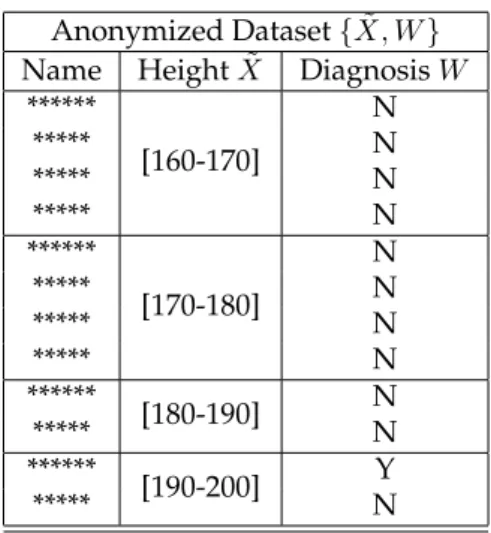
Anonymized Dataset{X, W˜ }
Name HeightX˜ DiagnosisW ******
[160-170]
N
***** N
***** N
***** N
******
[170-180]
N
***** N
***** N
***** N
******
[180-190] N
***** N
******
[190-200] Y
***** N
Table 3: Anonymized dataset.
3
Information theoretic Risk Metrics
Before entering in the details of the different privacy metrics, let us deduce a general rela-tion between the informarela-tion about the sensitive attributes and the quasi-identifiers before,
QIs can be generally represented as a function betweenX andX˜ 1for the data processing
inequality of the mutual information, we have:
I(W,X˜)≤I(W, X) (4)
Let us consider the different privacy metrics in terms of information theory.
• k-anonymity. In case of suppression and generalization, we have that a single QI group in the anonymized databasex˜can correspond to a number,Nx˜ of records in
the original tableX. Accordingly, the probability of re-identifying a recordxgivenx˜ is simply:p(x|˜x) = 1/Nx, and˜ k-anonymity reads:
H(X|x)˜ ≥log2k (5)
for eachx˜∈X˜. In terms of one-symbol specific informationI2, it reads
I2(X,x)˜ ≡H(X)−H(X|x)˜ ≤log2
N
k (6)
whereNis the number of tuples in the original datasetX(assumed different).I2(X,x)˜
measures the identity disclosure risk for a single record. Eq. 5 holds also in case of perturbative masking [4], thereforeI2can be used for any kind of masking
transfor-mations.
Averaging Eq. 6 overX˜ we get:
I(X,X˜)≤log2
N k
So, the mutual information can be used as a risk indicator for identity disclosure [13], but we have to stress that this condition does not guarantee thek-anonymity QI group ˜
x, i.e., it is necessary but not sufficient.
• t-closeness condition requires:
D(p(w|x)˜ ||p(w))≡ X
w∈W
p(w|x) log˜ 2
p(w|x)˜
p(w) ≤t (7)
for each x˜ ∈ X˜. This is equivalent to the one-symbol specific informationI1
(sur-prise), i.e.,
I1(W,x)˜ ≡
X
w∈W
p(w|x) log˜ 2
p(w|x)˜
p(w) ≤t (8)
I1(W,x)˜ is a measure of attribute disclosure risk for a QI groupx˜, as difference
be-tween the prior belief aboutW from the knowledge of the entire distributionp(w), and the posterior beliefp(w|x)˜ after having observedx˜and the corresponding sensi-tive attributes. Averaging over the setX˜ we get an estimation of the disclosure risk (based on t-closeness) for the whole set [24],
I(W,X˜)≡ X
˜
x∈X˜
p(˜x) X
w∈W
p(w|x) log˜ 2
p(w|x)˜
p(w) ≤t (9)
Again, this is necessary but not a sufficient condition to have t-closeness table, since this condition requires to havet-closeness for eachx˜.
• ℓ-diversity condition, in terms of entropy, reads:
H(W|˜x)≥log2ℓ
for each QI groupx˜ ∈X˜. It can be expressed in terms of one-symbol specific infor-mationI2,
I2(W,x)˜ ≡H(W)−H(W|x)˜ ≤H(W)−log2ℓ (10)
I2(W,x)˜ is a measure of attribute disclosure risk for a QI group ˜x, as reduction of
uncertainty between the prior distribution and the conditional distribution.
Averaging over the setX˜ we get an estimation of the average disclosure risk for the whole set [24].
I(W,X)˜ ≡H(W)−H(W|X)˜ ≤H(W)−log2ℓ (11)
This is theℓ-diversity condition on average. Again, this is necessary but a not suffi-cient condition to satisfyℓ-diversity for eachx˜. Note that, since the mutual informa-tion is a non-negative quantity,I(W,X)˜ ≥ 0, from Eq. 11 immediately follows that H(W)is an upper bound forlog2ℓ, i.e.,
log2ℓ≤H(W)
or equivalentlyℓ≤ℓmax≡2H(W).
Eqs. 9, 11 suggest a way to compare the two risk parametersℓandt. Indeed, if we equalize the maximal contribution to information ofℓandt, we can derive the following relation:
ℓt= 2H(W)−t (12)
ℓttells us, for a givent, what theequivalentvalueℓis, i.e., the value ofℓthat has the same impact on the information. The advantage of Eq. 12 is that it allows us to express the value oftparameter, which it is often hard to set, in terms ofℓ, that has a much more intuitive meaning.
In summary, for any anonymized dataset which satisfiesℓ-diversity andt-closeness, the following average conditions arenecessary:
I(W,X˜)≤I(W, X)
I(W,X˜)≤t
I(W,X˜)≤H(W)−log2ℓ
(13)
whereas thenecessaryandsufficientconditions are:
I1(W,˜x)≤t
I2(W,˜x)≤H(W)−log2ℓ
(14) for eachx˜∈X˜.
For setting the risk parameters, we derived lower and upper bounds forℓ,
1≤ℓ≤ℓmax≡2H(W) (15)
and theℓtequivalent tot,
ℓt= 2H(W)−t
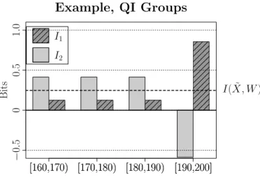
[160,170) [170,180) [180,190) [190,200]
Example, QI Groups
Bits
[160,170) [170,180) [180,190) [190,200] I2
I1
−
0
.
5
0
0
.
5
1
.
0
I( ˜X, W)
Figure 1: Values of information-based disclosure risk metrics: I1 (t-closeness) andI2 (ℓ
-diversity related) for the different entries in the anonymized database. Dashed line indi-cated mutual informationI( ˜X, W), i.e., the average ofI1andI2.
3.1
Example
To illustrate the qualitative and quantitative differences in the behavior oft-closeness and ℓ-diversity based risk metrics,I1andI2, let us consider a simple example. This example is
not realistic, but the aim is to show some basic features ofI1andI2without any additional
complexity. Let us take a medical database{X, W}(Table 2) containing three fields only: a unique identifier (name), a quasi-identifier (Height) and a sensitive attribute (Diagno-sis). In the released, anonymized dataset{X, W˜ }, Table 3, names are removed, the Height generalized in broader classes, and the sensitive attribute unchanged. Let us say that after this anonymization process, we have reached an acceptable level of identity and attribute disclosure risk as measured byI(X,X)˜ andI(W,X)˜ . But, if we analyze the contribution to this risk of single entries inX˜ in terms of symbol specific informationsI1,I2(see Fig. 1),
we observe:
• The distribution of risk shows large fluctuations, so the average is not a good repre-sentation of the risk level.
• The entries at risk (say, well above the average) depends on the risk measures used (I1 orI2). In other words, set of tuples (QI groups) largely at risk accordingI2 (ℓ
-diversity based) have low value ofI1(so they are acceptable from t-closeness point of
view), and vice versa.
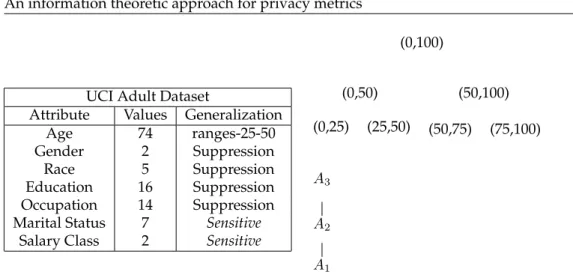
UCI Adult Dataset
Attribute Values Generalization
Age 74 ranges-25-50
Gender 2 Suppression
Race 5 Suppression
Education 16 Suppression
Occupation 14 Suppression Marital Status 7 Sensitive
Salary Class 2 Sensitive
(0,100)
(0,50) (0,25) (25,50)
(50,100) (50,75) (75,100)
A3
A2
A1
Table 4: Left. Summary of the anonymization methods. Right. Generalization hierarchy for age attribute: first level,A1, Age is generalized in25years range,A2in50years andA3
fully generalized. Un-generalized Age (A0) not shown.
(0,100)
(0,50) (0,35) (35,50)
(50,100) (50,60) (60,100)
A3
A2
A∗
1
]
Table 5: Generalization hierarchy for age attribute: first level, A∗
1, Age is generalized in
ranges of variable size, for minimizing information loss.A2in50years andA3fully
gener-alized. Un-generalized Age (A0) not shown.
4
Experiments
For testing our framework, we performed some numerical analysis on a relatively large dataset widely used in the research community. We ran our experiments on the Adult Database2from the UCI Machine Learning Repository, which contains32561tuples from
US Census data with15demographic and employment related variables. We removed the tuples with missing values, ending with30162usable tuples.
The choice of the identifiers, QIs, and sensitive attribute set, typically depends on the spe-cific domain. In particular, for QIs, they should include the attributes a possible attacker is more likely to have access to (e.g., using a phonebook or a census database) and for sensitive attribute to the application the anonymized data are used for. Generally speak-ing increasspeak-ing the number of QIs increases the risk, or results in strong anonymization impacting final data quality. In our experiments we limited the QIs to four attributes:
QI ≡ {Age, Gender, Race, Education}. The generalizations applied are summarized in
Ta-ble 4. In the census data the salary is typically chosen as sensitive attribute. In this dataset,
I( ˜X, W) H(W) -log2ℓ
t I(X, W)
Generalization: A2
Bits
0
0
.
2
0
.
4
0
.
6
0
.
8
[0,50) [50,100]
Gen.:A2, QI Groups
Bits
[0,50) [50,100]
I2 I1
0
0
.
4
0
.
8
1
.
2
H(W )-log2(2.7)
t=0.55
Figure 2: Left: Mutual informationI( ˜X, W)between the anonymized QIs and the sensitive attribute (black bar), thetvalue (shaded dark gray bar),ℓ-diversity threshold for informa-tion (light gray bar), and the mutual informainforma-tion between the original QIs and the sensitive attributes (white bar). Right: information contributions in terms ofI1 (shaded dark gray
bar) andI2(light gray bar) for theA2QI groups. Straight line indicates thetthreshold, for I1, witht= 0.55. Dashed line indicates theℓ-diversity threshold forI2(ℓ= 2.7).
salary attribute can assume two values>50kand<50k, and the entropy of this attribute is quite small (H ≈0.80), limiting its effectiveness for demonstrating the different features of the privacy metrics. Therefore, for our tests, we used as sensitive attribute the Marital Status, which has7possible values and a larger entropy (H ≈1.85), which corresponds to a maximum value ofℓmax≈3.53.
Let us consider that we want to release this dataset, assuring that the privacy risk is under a certain threshold value, as measured bytandℓ.
We set these thresholds as following: ℓ = 2.7andt = 0.55. For setting theℓthreshold, we had to find a compromise between having a sufficient level of privacy, and the same time not impacting too much the quality of data. In particularℓvalues lower than2do not clearly provide much privacy, whereas, considering the maximum value ofℓmax ≈ 3.53, values larger than3need a strong anonymization, which removes most of the information. We sett in a way that its information contribution does not differ too much from theℓ contribution, for our analysis we choset= 0.55, which corresponds to a value ofℓt= 2.42 so differing of≃10%from the chosen value ofℓ.
For the anonymization step, we used as anonymizaton engine the UT Dallas Anonymiza-tion Toolbox [19], which implements Incognito algorithm fork-anonymity andℓ-diversity. This toolbox comprises an implementation of Incognito fort-closeness, too, but it measures tvalue against the Earth Moving distance (whereas we use Eq. 7), so we did not use it, and we verified thetvalue, according to our metric, on the anonymized dataset.
We run the anonymization engine using the transformations listed in Table 4(Left), and we obtained that the attributes{Gender, Race, Education}were suppressed (or fully gen-eralized) andAgegeneralized in two groups,A2(see Table 4(Right)).
I( ˜X, W) H(W) -log2ℓ
t I(X, W)
Generalization: A1
Bits
0
0
.
2
0
.
4
0
.
6
0
.
8
[0,25) [25,50) [50,75) [75,100]
Gen.:A1, QI Groups
Bits
[0,25) [25,50) [50,75) [75,100] I2 I1
0
0
.
4
0
.
8
1
.
2
H(W )-log2(2.7)
t=0.55
Figure 3: Left: Original mutual informationI( ˜X, W)(black bar), thetvalue (shaded dark gray bar), ℓ-diversity threshold (light gray bar), and the mutual information for anoyn-mized dataset (white bar). Right: information contributionsA1QI groups. For details see
the caption of Fig. 2
average information are fulfilled, and I( ˜X, W)(white bar) is lower than the other three bars. In Fig. 2(Right), we plot the information contributions in terms ofI1 andI2 for the
two QI groups. Both of them are lower than the corresponding thresholds fort (contin-uous line) andℓ, fulfilling the conditions expressed by Eqs. 14. In other words, for this anonymized dataset2.7-diversity and0.55-closeness are fulfilled.
On the other hand, the information loss is quite relevant≈88%(see white bar vs. black bar in Fig. 2(Left)), and it is typically desirable to preserve as much information as possible in the anonymization3. To this scope, we consider a weaker generalization on{Age}attribute,
i.e., one single levelA1instead of twoA2of the previous case.
In Fig. 3(Left) we show the amount of information I( ˜X, W) (white bar) left after the anonymization, and (as in the previous case) we compared it with Eq. 11, thetvalue, and the original informationI(X, W). We can see thatI( ˜X, W)is lower than the other bars, i.e., the conditions expressed by Eqs. 13 are fulfilled. These conditions are necessary but not sufficient for havingℓ-diversity and t-closeness enforced. Indeed, if we analyze the contribution of the level of QI group, Fig. 2(Right), we observe that two groups (labeled [0,25)and[75,100]) do not satisfy thetcloseness condition (continuous line), and one of them,[0,25), does not satisfyℓ-diversity condition (dashed line). Note, as in the example of Section 3.1,[75,100]group has a very different risk profile depending whether we uset orℓ, i.e., very risky fromt-closeness point of view, and pretty safe forℓ-diversity.
In short, although the conditions on the average are satisfied, the same is not true for each ˜
x, QI group, so the dataset is neither2.7-diverse nor satisfies0.55-closeness.
We identified the two QI groups that do not fulfill the privacy requirements, the next step is trying to increase the size of these outlier groups for reducing the privacy risk (both in terms ofℓ and t). To this scope, we modified the first level of the generalization A1
3Note that here we try to maximize the informationI( ˜X, W), or minimize the information loss, whereas, as
I( ˜X, W) H(W) -log2ℓ
t I(X, W)
Generalization: A∗1
Bits
0
0
.
2
0
.
4
0
.
6
0
.
8
[0,35) [35,50) [50,60) [60,100]
Gen.:A∗1, QI Groups
Bits
[0,35) [35,50) [50,60) [60,100] I2 I1
0
0
.
4
0
.
8
1
.
2
H(W )-log2(2.7)
t=0.55
Figure 4: Left: Original mutual informationI( ˜X, W)(black bar), thetvalue (shaded dark gray bar), ℓ-diversity threshold (light gray bar), and the mutual information for anoyn-mized dataset (white bar). Right: information contributionsA∗
1QI groups. For details see
the caption of Fig. 2
hierarchy for age attribute, in particular we run an heuristic search for the optimal size of the two groups, which maximizes the informationI( ˜X, W), and satisfies thet-closeness and ℓ-diversity requirements. The resulted generalization A∗
1 is reported in Table 5. In
Fig. 4, we plotted, as in the previous cases, the mutual informationI( ˜X, W)compared to ℓandtthresholds and to the original informationI(X, W). On the right panel, we show I1andI2for each QI group compared to the risk thresholds. We can see ast-closeness and ℓ-diversity conditions are satisfied, and that we were able to preserve a larger amount of information compared toA2, Fig. 2, (we do not considerA1, since it does not satisfy our
privacy requirements), indeed the information loss was reduced to≈55%, compared to≈
88%ofA2, and in terms of information we haveI( ˜X, W) = 0.34forA∗1vs.I( ˜X, W) = 0.09
forA2.
In summary in our numerical analysis, using a census dataset, we showed the main fea-tures of information-based privacy metrics, including their application for setting risk pa-rameters, and how they can be used to reduce the information loss in the anonymization process.
5
Conclusions and Future Works
all the tools of information theory for optimizing the privacy constraints, and, possibly, utility. The last point can be technically difficult in many cases, because expressing condi-tions on particular records largely increases the complexity of the optimization problem. Indeed, Eq. 14 must hold for each QI group, resulting in large number of constraints, so making difficult to obtain analytical results and even numerical solutions. Clearly, this is a relevant question to address in the near future, and, in particular, it is important to test the applicability of our approach to realistic cases.
Another possible extension is considering other data release scenarios, and the corre-sponding privacy models. For example, if we examine the scenario where the data pub-lisher knowns in advance the data mining tasks, we can consider thedifferential privacy
notion [15]. In a nutshell, the idea of differential privacy model, calledǫ-differential privacy, is to guarantee that small changes (one record) in the original database has a limited im-pact on the outcome of any statistical analysis on the data. More formally, let us consider a databaseX0 (we do not distinguish between identifiers and sensitive attributes, so we
will use X0 to indicate the whole original database), and a randomized functionF that
has as output a real number4, for example composed by a query on the original database
that returns a numerical value plus an appropriately chosen random noise. We say that the random functionF ensuresǫ-differential privacy if for all the datasetsX0
sup X∈X
sup s∈S
lnp(F =s|X0)
p(F=s|X)
≤ǫ (16)
whereX ≡ {X|δ(X0, X) ≤ 1}, i.e., the set of databases differing for at most one record
fromX0(δis the Hamming distance),S ≡Range(F), where Range(F) is the set of possible
outputs of the randomized functionF, andǫis the privacy parameter. The closerǫis to0, the stronger privacy is guaranteed (for a discussion onǫsee [16]).
A good candidate for expressing theǫ-differential privacy as an information metric is the surprise,I1, of the databaseX0(not of a single record, as used above), i.e.
I1(F, X0)≡
X
s∈S
p(s|X0) log2
p(s|X0)
p(s) ≤θǫ (17)
with
p(s) = X
X∈X
p(s|X)p(X)
andθǫis a parameter related to theǫof Eq. 16
Note that the condition expressed by Eq. 17 is different from Eq. 16, since in the first case we compare the probabilityp(s|X0)of having a certain outcomesfrom the analysis of the
databaseX, with the average outcome over “similar” databases,p(s), and then we average over all the possible outcomes. Whereas, in the originalǫ-differential privacy, we compare p(s|X0)directly withp(s|X)(so, not with the average), and we take the maximum overs
and over all the neighbor databases. Therefore, the latter condition is more conservative. The formal relationship between Eq. 17 and Eq. 16, and between the corresponding thresh-olds, θǫ and ǫ, as well as a more detailed analysis of possible advantages of expressing differential privacy in terms of information theory have to be investigated in future works.
4For sake of simplicity, we consider here a single functionF that takes values inR, but the same analysis
can be applied to a functionFwhich takes values inRn
Acknowledgements
The research leading to these results has received funding from the European Community’s Seventh Framework Programme (FP7/2007-2013) under grant agreement no. 216483. I also thank Stuart Short for the careful reading of the manuscript.
References
[1] Dakshi Agrawal and Charu C. Aggarwal. On the design and quantification of privacy preserv-ing data minpreserv-ing algorithms. InPODS ’01: Proceedings of the twentieth ACM SIGMOD-SIGACT-SIGART symposium on Principles of database systems, pages 247–255, New York, NY, USA, 2001. ACM.
[2] J. Bennett and S. Lanning. The Netflix Prize.KDD Cup and Workshop, 2007.
[3] M. Bezzi, I. Samengo, S. Leutgeb, and S.J. Mizumori. Measuring information spatial densities.
Neural computation, 14(2):405–420, 2002.
[4] Michele Bezzi. An entropy-based method for measuring anonymity. In Proceedings of the IEEE/CreateNet SECOVAL Workshop on the Value of Security through Collaboration, pages 28–32, Nice, France, September 2007.
[5] Michele Bezzi. Quantifying the information transmitted in a single stimulus. Biosystems, 89(1-3):4–9, May 2007 (http://arxiv.org/abs/q-bio/0601038).
[6] Michele Bezzi. Expressing privacy metrics as one-symbol information. InEDBT ’10: Proceedings of the 2010 EDBT Workshops, pages 1–5, New York, NY, USA, 2010. ACM.
[7] N. Blachman. The amount of information that y gives about X.IEEE Transactions on Information Theory, 14(1):27–31, 1968.
[8] D.A. Butts. How much information is associated with a particular stimulus? Network: Compu-tation in Neural Systems, 14(2):177–187, 2003.
[9] D.M. Carlisle, M.L. Rodrian, and C.L. Diamond. California inpatient data reporting man-ual, medical information reporting for california. Technical report, Technical report, Office of Statewide Health Planning and Development, 2007.
[10] T. Dalenius. Finding a needle in a haystack-or identifying anonymous census record. Journal of Official Statistics, 2(3):329–336, 1986.
[11] AG DeWaal and L. Willenborg. Information loss through global recoding and local suppression.
Netherlands Official Statistics, 14:17–20, 1999.
[12] M.R. DeWeese and M. Meister. How to measure the information gained from one symbol.
Network: Comput. Neural Syst, 10:325–340, 1999.
[13] J. Domingo-Ferrer and D. Rebollo-Monedero. Measuring Risk and Utility of Anonymized Data Using Information Theory. International workshop on privacy and anonymity in the information society (PAIS 2009), 2009.
[14] GT Duncan, S. Keller-McNulty, and SL Stokes. Disclosure risk versus data utility: The RU confidentiality map.Technical paper, Los Alamos National Laboratory, Los Alamos, NM, 2001. [15] Cynthia Dwork. Differential privacy. In Michele Bugliesi, Bart Preneel, Vladimiro Sassone, and
Ingo Wegener, editors,Automata, Languages and Programming, volume 4052 ofLecture Notes in Computer Science, pages 1–12. Springer Berlin / Heidelberg, 2006.
[17] R. M. Fano. Transmission of Information; A Statistical Theory of Communications. MIT University Press, New York, NY, USA, 1961.
[18] Benjamin C. M. Fung, Ke Wang, Rui Chen, and Philip S. Yu. Privacy-preserving data publishing: A survey of recent developments.ACM Comput. Surv., 42(4):1–53, 2010.
[19] Ali Inan, Murat Kantarcioglu, and Elisa Bertino. Using anonymized data for classification. In
ICDE ’09: Proceedings of the 2009 IEEE International Conference on Data Engineering, pages 429–440, Washington, DC, USA, 2009. IEEE Computer Society.
[20] Ninghui Li, Tiancheng Li, and S. Venkatasubramanian. t-closeness: Privacy beyond k-anonymity and l-diversity. InData Engineering, 2007. ICDE 2007. IEEE 23rd International Confer-ence on, pages 106–115, April 2007.
[21] T. Li and N. Li. On the tradeoff between privacy and utility in data publishing. InProceedings of the 15th ACM SIGKDD international conference on Knowledge discovery and data mining, pages 517–526. ACM New York, NY, USA, 2009.
[22] Ashwin Machanavajjhala, Johannes Gehrke, Daniel Kifer, and Muthuramakrishnan Venkita-subramaniam. l-diversity: Privacy beyond k-anonymity. InICDE ’06: Proceedings of the 22nd International Conference on Data Engineering (ICDE’06), page 24, Washington, DC, USA, 2006. IEEE Computer Society.
[23] Frank McSherry and Kunal Talwar. Mechanism design via differential privacy. Foundations of Computer Science, Annual IEEE Symposium on, 0:94–103, 2007.
[24] David Rebollo-Monedero, Jordi Forne, and Josep Domingo-Ferrer. From t-closeness-like pri-vacy to postrandomization via information theory. IEEE Transactions on Knowledge and Data Engineering, 99(1), 2009.
[25] Pierangela Samarati. Protecting respondents’ identities in microdata release.IEEE Trans. Knowl. Data Eng., 13(6):1010–1027, 2001.
[26] C. E. Shannon. A mathematical theory of communication. Bell System Tech. J., 27:379–423,623– 656, 1948.