DINAMICA VIRTUAL MACHINE PARA
BRUNO MORAIS FERREIRA
DINAMICA VIRTUAL MACHINE PARA
GEOCIÊNCIAS
Dissertação apresentada ao Programa de Pós-Graduação em Ciência da Computação do Instituto de Ciências Exatas da Univer-sidade Federal de Minas Gerais como req-uisito parcial para a obtenção do grau de Mestre em Ciência da Computação.
Orientador: Fernando Magno Quintão Pereira
Belo Horizonte
BRUNO MORAIS FERREIRA
THE DINAMICA VIRTUAL MACHINE FOR
GEOSCIENCES
Dissertation presented to the Graduate Program in Computer Science of the Uni-versidade Federal de Minas Gerais. Detamento de Ciência da Computação. in par-tial fulfillment of the requirements for the degree of Master in Computer Science.
Advisor: Fernando Magno Quintão Pereira
Belo Horizonte
c
2015, Bruno Morais Ferreira. Todos os direitos reservados.
Ferreira, Bruno Morais
F383d The dinamica virtual machine for geosciences / Bruno Morais Ferreira. — Belo Horizonte, 2015
xxii, 66 f. : il. ; 29cm
Dissertação (mestrado) — Universidade Federal de Minas Gerais. Departamento de Ciência da
Computação.
Orientador: Fernando Magno Quintão Pereira
1. Computação — Teses. 2. Modelagem ambiental — Teses. 3. Linguagens de programação funcional — Teses. I. Orientador. II. Título.
Dedico este trabalho aos meus pais, avós, esposa e amigos.
Acknowledgments
Agradeço aos meus pais por investirem na minha educação, aos meus avós pelo duro trabalho e infinita inspiração, à minha esposa pelo amor e apoio constantes e aos meus amigos pela alegria e suporte. Agradeço ao meu orientador pela ajuda no trabalho e pela inspiração que sua atitude proporciona. Agradeço ao Centro de Sensoriamento Remoto da UFMG e a todos os colegas que ali trabalham. Por fim, agradeço a Deus por tudo.
Resumo
Este trabalho descreve a DinamicaVM, a máquina virtual para execução de aplicações desenvolvidas em Dinamica EGO. Dinamica EGO é uma plataforma utilizada em mod-elagem e simulação ambiental. Por detrás da sua biblioteca de elementos visuais em modo gráfico, Dinamica EGO roda em cima de uma máquina virtual. Esta máquina - DinamicaVM - oferece aos desenvolvedores um rico conjunto de instruções, com ele-mentos como o "map" e "reduce", que são típicos no mundo de linguagens funcionais e paralelismo. Garantir que estes componentes, muito expressivos, trabalhem juntos de forma eficiente é uma tarefa desafiadora. O ambiente de execução do Dinamica vence este desafio através de um conjunto de otimizações, emprestando ideias de linguagens de programação funcional, levando ao comportamento específico esperado em progra-mas de alta performance para modelagem ambiental. Como mostramos neste trabalho algumas dessas otimizações levam speedups de quase 100 vezes, e são fundamentais para o desempenho e qualidade de uma das ferramentas de modelagem ambiental mais utilizadas do mundo.
Palavras-chave: Fluxo de Dados, Linguagem de Domínio Específico, Modelagem Ambiental.
Abstract
This work describes DinamicaVM, the virtual machine that runs applications devel-oped in Dinamica EGO. Dinamica EGO is a framework used in the development of geomodeling applications. Behind its multitude of visual modes and graphic elements, Dinamica EGO runs on top of a virtual machine. This machine - DinamicaVM - of-fers developers a rich instruction set architecture, featuring elements such as map and reduce, which are typical in the functional/parallel world. Ensuring that these very expressive components work together efficiently is a challenging endeavour. Dinamica’s runtime addresses this challenge through a suite of optimizations, which borrows ideas from functional programming languages, and leverages specific behavior expected in geo-scientific programs. As we show in this work some of these optimizations deliver speedups of almost 100x, and are key to the industrial-quality performance of one of the world’s most widely used geomodeling tools.
Palavras-chave: Dataflow, Domain Specific Languages, Geomodeling.
List of Figures
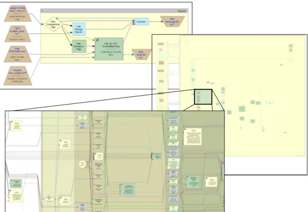
1.1 A typical screenshot of an EGO Script program. Components can be ex-panded in more complex views by the user. . . 2
1.2 The implementation of Conway’s Game of Life in Dinamica EGO. Letters in parentheses are not part of the original screenshot. . . 4
3.1 A schematic view of Dinamica EGO’s Virtual Machine. . . 20
3.2 The four high-level functors in DinamicaVM’s instruction set architecture. (a) Apply; (b) Reduce; (c) Window; (d) While. . . 21 3.3 (a) The four loops that implement the chaotic iterations of theCalcCostMap
functor. (b) Dependencies between tiles in the first loop: upper-left to lower-right. (c) Tiles with the same number can be processed together in the first loop. (d) Example of cost map that Dinamica produces. . . 25
4.1 Example of fusion. The Apply operator is always the increment function, and theReduce operator is the sum of integers. . . 28 4.2 The three-lines cache. The dashed arrows show line pointers in the previous
iteration of Window. The solid arrows show the pointers in the current iteration. (a) Input map. (b) Cached lines. (c) Center of 3×3 window. . . 30 4.3 Performance gain due to prefetching in an image smoother. . . 31
4.4 Performance gains in Conway’s Game of Life (Section 1.1) due to unrolling and prefetching. X-axis is the number of generations of the automaton, and Y-axis is runtime, in msecs. . . 32
5.1 An EGO Script program that finds the average slope of the cities that form a certain region. The parallel bars denote places where the original implementation of Dinamica EGO replicates data. . . 36 5.2 Two examples in which copies are necessary. . . 38
5.3 The operational semantics of µ-Ego. . . 39
5.4 Canonical evaluation of an µ-Ego program. (a) The graph formed by the components. (b) The scheduling. (c) The final configuration of Σ. (d) The final configuration of T. . . 40 5.5 Evaluation of an optimized µ-Ego program. . . 41 5.6 Evaluation of an µ-Ego program that does not produce a canonical result. 41 5.7 Reducing Smfs to interval graph coloring for schedulings without
back-edges. (a) The input µ-Ego( program. (b) The input scheduling. (c) The corresponding intervals. The integers on the left are the orderings of each component in the scheduling. . . 43 5.8 Reducing Smfs to circular-arc graph coloring for general schedulings. (a)
The input arcs. (b) The corresponding µ-Ego program. . . 44 5.9 An example that illustrates how Sethi’s programs can be translated to µ
-Egoscripts. (a) The e-DAG that represents the expression(c×x+b)×x+a. (b) A solution to Sethi’s game. (c) The correspondingµ-Ego program. . . 46 5.10 Inference rules that define our data-flow analysis. . . 47 5.11 The result of the data-flow analysis on the program seen in Figure 5.1. . . 48 5.12 Criteria to replicate data in Ego Script programs. . . 49 5.13 Hilltop detection. (a) Height map. (b) Normalized map. (c) Extracted
discrete regions. . . 52
List of Tables
5.1 V: Vertical resolution(m). D: Number of dynamic copies without optimiza-tion. Tu: Execution time without optimization (s). To: Execution time
with optimization (s). R: Execution time ratio. . . 53 5.2 MS: size of map’s side, in number of cells. Each map is a square matrix.
D: Number of dynamic copies without optimization. Tu: Execution time
without optimization (s). To: Execution time with optimization (s). R:
Execution time ratio. . . 54
Contents
Acknowledgments xi
Resumo xiii
Abstract xv
List of Figures xvii
List of Tables xix
1 Introduction 1
1.1 Dinamica in One Example . . . 4
2 Literature Review 7 2.1 Other Geomodeling Tools . . . 7
2.2 Dataflow Programming Languages . . . 9
2.3 Ensuring referential transparency in the presence of destructive updates 14 3 The Dinamica Virtual Machine 19 3.1 Apply . . . 20
3.2 Reduce . . . 22
3.3 Window . . . 23
3.4 While . . . 23
3.5 Specific Components . . . 24
4 Optimizations 27 4.1 Fusion . . . 28
4.2 Window Optimizations . . . 29
4.2.1 Prefetching . . . 30
4.2.2 Performance Improvement due to Pre-fetching . . . 31
4.2.3 Unrolling . . . 32
5 A Semantics Model of EGO Script and the Copy Elimination
Op-timization 35
5.1 Dinamica EGO in Another Example . . . 36 5.2 The Core Semantics . . . 38 5.3 The Copy Elimination Problem . . . 39 5.3.1 SMFS has polynomial solution for schedulings with no back-edges 41 5.3.2 SMFS is NP-complete for general programs with fixed scheduling. 43 5.3.3 Copy replication is NP-complete with open scheduling on DAGs. 44 5.4 Copy Minimization . . . 46 5.4.1 Data-Flow Analysis . . . 47 5.4.2 Criteria to Eliminate Copies . . . 48 5.4.3 Correctness . . . 50 5.5 Experiments . . . 51 5.5.1 First Case Study: Hilltop Calculation . . . 52 5.5.2 Second Case Study: Map Statistical Analysis . . . 53
6 Conclusion 55
6.1 Limitations and Future Work . . . 56 6.2 Closing Remarks . . . 56
Bibliography 59
Chapter 1
Introduction
Computer Science have been playing an important role in several fields of science and this is not different with environmental sciences. The need to understand how the planet Earth works is the greatest motivation to the development of new methods, techniques, algorithms. With the advent of remote sensing a great amount of data about the Earth’s surface became available. Apply these methods and techniques in models and simulations that use this great amount of data is a challenging endeavour and is in this context that Dinamica EGO emerges.
Dinamica EGO is a framework that supports the development of geomodeling ap-plications [Soares-Filho et al., 2002, 2009, 2013]. It was first released in 1998, and since then it has grown to enjoy international recognition as an effective and useful framework for geomodeling. It has been used to model carbon emission and deforestation [Carlson et al., 2012; Nepstad et al., 2009], biodiversity loss [Pérez-Vega et al., 2012], urban-ization and climate change [Huong and Pathirana, 2011], emission reduction [Hajek et al., 2011] and urban growth [Thapa and Murayama, 2011]. Testimony of Dinamica’s maturity are the intergovernmental collaborations where it is used. Among its appli-cation to public policies in collaboration with governmental institutions in Brazil and abroad we cite the World Bank and the United Nations Development Programme. For instance, the REDD project, which integrates state departments from Bolivia, Peru and Brazil, is using Dinamica to map the southwestern Amazon1
. As another example of relevant use, Dinamica’s simulation of the environmental impact of the Santarém-Cuiabá Interstate (BR 163) has been key to lead the Brazilian government to create a national preservation area along this highway2
. Finally, SimAmazonia, a large effort to model climate change in the Amazon Basin using Dinamica EGO [Soares-Filho et al.,
1
http://csr.ufmg.br/map/
2
http://www.csr.ufmg.br/dinamica/applications/cuiaba- santarem.html
2 Chapter 1. Introduction
Figure 1.1. A typical screenshot of an EGO Script program. Components can be expanded in more complex views by the user.
2006]3 .
Dinamica EGO - EGO stands for Environment for Geoprocessing Objects - was created as an assemblage of components implemented in C++, called functors, which represent typical map algebra operations [Tomlin, 1990] and other other specific al-gorithms. Figure 1.1 shows a screenshot of an application implemented in Dinamica. What this application does is immaterial for this presentation. Each functor has a num-ber of inputs, and produces a numnum-ber of outputs. The edges that interconnect these ports determine how data flows in a Dinamica’s application. The original Dinamica’s design had one fundamental disadvantage: functors were complex components imple-menting complete algorithms. Given this coarse granularity, whenever Dinamica’s users needed to implement new behaviors, they had to ask the developers of that framework to code new functors.
To circumvent this shortcoming, we have implemented, from 2012 and 2014, Di-namicaVM, a virtual machine designed to make the Dinamica framework more flexible.
3
3
The goal of this work is to describe this virtual machine and its companion program-ming environment. DinamicaVM contains an instruction set, a library of external components, a scheduler, a garbage collector and an optimizer. The instruction set is built around four functors: map,Reduce, Window and While, plus functors that define simple operations such as And, Add, Mul, etc. Map and Reduce are typical functional-oriented patterns, today heavily used in parallel programming [Dean and Ghemawat, 2008]. Henceforth, to avoid confusion with the maps used as Dinamica’s main data type, we shall call the map functor Apply. Window returns a neighbourhood within a map. Whilereceives a map, and a state, and return zero or more new states which are a function of the input map.
Dinamica’s main data type is theraster map. Raster maps (orrasters) are regular grids of pixels called cells. A raster has a cell type wich can be float or integer with variable bit length. Map files may provide a variety of metadata that can describe map projection, coordinate systems, ellipsoids, datums and other geographic information. It can be seen as a 2D matrix of data along with a set of georeferencing information.
Tomlin [1990] described an algebra for the manipulation of geographic data and with a set of algebraic operations it is possible to produce a new raster map from other input rasters. The transformations proposed by this map algebra are separated into the groups: local, focal, global, and zonal. Each one differs from the other by the number of the cells a transformation works over: individual cells, neighbourhoods, entire maps or all cells with the same value.
It is not the goal of this work to describe the relation of Dinamica EGO and Tomlin’s algebra, but to present our virtual machine for the current Dinamica EGO environment. As we state in Chapter 3, Dinamica provides general operators, but also specific components that are not present in map algebra. Indeed, it is possible to describe all map algebra transformations using Dinamica’s operators, but the opposite is not true. We do not provide a proof for this statement since our focus is on the DinamicaVM components and its optimizations.
4 Chapter 1. Introduction
(a.1)
(a.2)
(a.3) (b) (c)
(c.2) (c.1)
(d) (e)
(b.1)
(f)
Figure 1.2. The implementation of Conway’s Game of Life in Dinamica EGO. Letters in parentheses are not part of the original screenshot.
datasets dramatically, and in some cases, can deliver speedups of over 100x.
In Chapter 3 we introduce, the semantics of each of the four core building-blocks of Dinamica’s applications. The architecture that these four components define finds no equal in other systems built with similar purpose, as we explain in Chapter 2. In Chapter 4 we describe the optimizations that ensure that these components run effi-ciently. Some of these optimizations are not new: they have already being implemented in functional languages [Wadler, 1988]. Nevertheless, we revisit them under the light of a virtual machine customized to handle maps and tables that represent geographic entities, i.e. a domain specific language. For instance, even though cache optimiza-tions are well studied, we claim the cache-related transformaoptimiza-tions from Section 4.2 as original contributions of this work. A paper about these techniques and the virtual machine description has just been submitted. Furthermore, our techniques to address the tension between parallelism and memory allocation, which we address in Chapter 5, have been described for the first time in our paper [Ferreira et al., 2012] and improved since it was published.
1.1
Dinamica in One Example
In this section we present Dinamica EGO through an example application. This ex-ample uses the core components of our virtual machine that we describe in Chapter 3. It is possible to note how these components can be combined to build a program in the Dinamica EGO environment. More examples can be found in the Dinamica EGO Guidebook 4
.
We illustrate the basic elements of Dinamica EGO via the implementation of Conway’s Game of Life [Gardner, 1970]. Figure 1.2 shows a screenshot of this
imple-4
1.1. Dinamica in One Example 5
mentation. The game happens on a two-dimensional grid of square cells. Each cell can be either active or inactive. The state of all the cells in a grid determine a generation of the game. Generation g + 1 is a function of generation g. The state of cell i at generation g+ 1 is determined by the state of this cell’s neighbours, at generation g. The neighbourhood of a cell i is the 3×3 grid centered at i, excluding i itself. If this neighbourhood contains 2 or 3 active cells, i will be active in the next generation, otherwise, it will be inactive. Conway’s Game of life is the canonical example of cellu-lar automaton. Dinamica uses, among other techniques, different cellucellu-lar automata to model land evolution due to human occupation [Soares-Filho et al., 2002].
The application in Figure 1.2 reads two inputs: an original map (a.1), plus an integer indicating how many generations of the game will be produced (a.2). Its output is the map after the final generation (a.3). ARepeatfunctor (b) produces the successive generations of the game. Repeat is a specialization of a more general functor called
While, which we describe in Section 3.4. Repeatmay either read a new map, or work on data that it sends back to its input port. This feedbacking is implemented by a functor called Multiplexer (b.1). Multiplexers are equivalent to the φ-functions so ubiquitous in compiler analyses and optimizations [Cytron et al., 1991].
We use an Apply functor (c) to produce generation g + 1 of the game, given generation g. This component applies some operation on each cell of the input map according to an iterating index (c.1). This operator does not work in-place, unless the runtime environment optimizes it, as we will see in Chapter 5. That is, Apply’s output is a copy of the input map. In this particular example, we are using each Apply’s index
i to derive a Window (e) of 3×3 cells centered at i. A Reduce operator sums up the number of active cells on each neighbourhood. If this neighbourhood contains 2 or 3 active cells, then i will be active in the next generation, otherwise it will be inactive.
Some of the functors used in this example deal with data-structures. For instance,
Window reads a map, plus an index, and returns a neighbourhood within the map. Other functors operate on individual data. For instance, theif container (f) implements a conditional expression made of several smaller components, which we have not shown for the sake of readability. These components, e.g., Equal, And, Or and LessThan, implement unary and binary operations. Users program applications in Dinamica EGO by combining these operators. In particular, the control flow of a Dinamica EGO program is determined by how the different instances of Apply, Reduce, Window
Chapter 2
Literature Review
In this chapter we state related work present in the literature. We divide the relations in three areas. First we approach other geomodeling tools. Secondly, we give the reader an overview to other dataflow programming languages. Last, we present how the literature have been ensuring referential transparency in the presence of destructive updates. The latter is important due to our copy minimization optimization described in Chapter 5.
2.1
Other Geomodeling Tools
There exist many different tools that support the development of land use models. Some of them enjoy commercial success; others are popular in the academia. We are aware of four frameworks having a moderate to large user base that might compete with Dinamica in the geomodeling niche: ArcGIS1
, Idrisi2
, Metronamica3
and PCRaster4 . A direct comparison between all these tools is not possible, because they use different algorithms to perform simulations. Furthermore, there is not a common benchmark suite that they all can handle. Nevertheless, there exist a few limited studies comparing some of these tools. As an example, Pérez-Vega et al. [2012] have compared Dinamica and Idrisi, not from a performance perspective, but from the point of view of the accu-racy of each modeling algorithm. Dinamica is substantially faster, and more accurate in some situations. Idrisi’s algorithm, based on neural networks, is more accurate in others. Mas et al. [2014] compared Dinamica EGO in relation to CLUE-S and two Idrisi models. It presents the possibilities and limits of each software regarding the
1
http://www.esri.com/software/arcgis
2
http://clarklabs.org/
3
http://www.metronamica.nl/
4
http://pcraster.geo.uu.nl/
8 Chapter 2. Literature Review
modeling process. Flexibility and user friendliness is also considered. Furthermore, a virtual case study is presented to illustrate the applications.
Metronamica [RIKS, 2012; van Delden et al., 2005] is a set of simulation models that run coupled to the Geonamica software environment. It is not as verstile as a programming language, but provides several functionalities: a land use model, a zoning tool, regional model, a set of spatial indicators, transport, macro-economics and demographics. Users have been developing these and other kind of models in Dinamica’s framework.
PCRaster [Karssenberg et al., 2010] is a software framework used to build a vari-ety of environmental models (geography, hydrology, ecology, rainfall-runoff, vegetation competition, slope stability, etc). It allows data assimilation in addition to process-based stochastic spatio-temporal modeling. It provides a script language to the de-velopment of models by the user and also building blocks and analytical functions for manipulating raster GIS maps. This script language is called PCRcalc [Wesselung et al., 1996] and give to the user a library of operations for model construction. A Python extension is also supported for a more advanced development. PCRcalc is sim-ilar to the EGO Script textual language, but PCRaster does not have a graphical user interface for interactive programming. Similarly to Dinamica’s MapViewer, PCRaster deploys a data visualization tool called Aguila [Pebesma et al., 2007].
2.2. Dataflow Programming Languages 9
is obtained combining the information of each transition they have a more precise result with LCM. The authors attribute this better result to the neural networks. These “are able to express the simultaneous change potential to various land cover types more adequately than individual probabilities obtained through the weights of evidence method.” On the other hand, it is hard to use if a variety of simulation scenarios is pursued. The Land Change Modeler is limited in this situation because it is hard to modify the relationship between explanatory variables and change potential in the model. Several variables are used to calibrate both models: slope, distance to settlements, distance to roads, distance to agriculture, and land tenure.
Mas et al. [2014] presents a broader comparison between Dinamica, CLUE-S and two models present in Idrisi: MARKOV and the Land Change Modeler. CA-MARKOV [Paegelow and Olmedo, 2005] uses Markov chain matrices in the modeling process in the first step of the model: determine the quatity of change. To allocate these changes, that is the second step, it uses cellular automata and suitability maps. CLUE-S (Conversion of Land Use and Its Effects at Small regional extent) [Verburg et al., 2002; Verburg and Overmars, 2009] simulates the competition and interactions between the different land use changes types and uses mainly logistic regressions to make analysis of location suitability for this. The authors point LCM and CLUE have a more rigid structure with a fixed LUCC modeling flow procedures, while Dinamica and CA-MARKOV due to the large library of operators. Moreover, regarding ease of use the authos claim that “programming [Dinamica and CA-MARKOV] is easy even for users without previous programming experience because a graphical interface is provided in which operators can be dragged and linked dynamically to integrate feedback and iterative operations”. Some user friendliness topics are presented describing available documentation, input files types, and OS support. Finally, a virtual case study shows each software modeling capabilities and accuracy.
2.2
Dataflow Programming Languages
10 Chapter 2. Literature Review
are not aware of any dataflow language that supports geomodeling and landuse sim-ulation in particular. However, this paradigm has been employed in the most varied domains, ranging from music [Levitt, 1986] to image processing [Tanimoto, 1990], and has achieved commercial success [Johnson and Jennings, 2001].
Dataflow programming languages emerged due to the necessity of a language for dataflow hardware architechtures [Whiting and Pascoe, 1994; Johnston et al., 2004]. Conventional imperative programming languages was hard to compile for these hard-wares. In turn, the first interest with dataflow architechtures was to explore massive parallelism. Researchers used to think that von Neumann hardware would not be able to achieve the same performance due to a global program counter and global updat-able memory. Although, these dataflow architectures never surpassed the von Neumann hardware due to a too fine grain execution model, among other aspects. Nevertheless, the dataflow concept and the dataflow languages remained due to is powerful abstrac-tion and sometimes enhanced productivity [Baroth and Hartsough, 1995]. There is a huge set of textual and visual dataflow languages. A selection of these is described next.
An MIT student, Weng [1975], has described one of the first dataflow languages: The Textual Data-Flow Language - TFDL. Its features are: compile time deadlock detection, translated into dataflow format, formalized semantics. No data structures were available and only two data types were present: Booleans and integers. Programs in TFDL are lists of modules that can be recursive, but iterations were not possible. Modules may have assignments, conditional statements or calls. Since it was the first effort to a textual description of dataflow graphs, TFDL become an important ref-erence for the development of other dataflow languages, including discussions about communicating modules and streams implementations.
LAU [Gelly, 1976; Comte et al., 1978] was a language developed for the LAU computer architechture based on the static dataflow model. A LAU program, with its data-driven semantics, have statements for simple assignment, parallel assignment using the expand operator, decision using the case expression, and iteration with the loopoperator (theoldkeyword was used to keep the single assingment rule). The ability to encapsulate data and operations was availabe, what is a feature present in object oriented languages. Thecreateoperator can be used to define an object attributes and operations.
2.2. Dataflow Programming Languages 11
visual components in a software. Usually, drawing the graph that represents the pro-gram where nodes are operations and edges are the paths for the data. We describe some dataflow visual programming languages next.
Davis [Davis, 1974, 1979] described the Data-Driven Nets (DDNs), a graphical language to program the DDM1 computer [Davis, 1978]. The programs consist of a collection of cells and a set of directed data paths interconnecting these cells within a cyclic graph structures. Data is typed and travels along these paths: message, vector, and scalar. DDN cells can be of different types in the DDMl computer machine language. Possible constructs are: procedure calls, conditionals, arbitration, iteration, synchronization, distribution of data items, and deterministic merging. Although a visual programming language, DDN is very low level as pointed by the author himself, and anyone should program directly in this language. However, key concepts could be presented without the use of a textual language (iteration, procedure calls, and conditional execution, e.g.).
Davis [Davis and Lowder, 1981] also described a higher level language called GPL. The intention was to create a more practical higher-level version of DDN. The authors tried to provide a system with intuitive clarity where the program is a graph itself and not just a representation of it. GPL programs have two types of functions, atomic and macrofunctions. The former are simpler indivisible functions and the latter can be expanded to subgraphs allowing structured programming. Macrofunctions also allows recursion. The GPL environment provide facilities for debugging, and visualization. If desired, text-based programming can be used. In these graphs, arcs are typed and handle tuples, files, and functions as values. It is believed that GPL was the first fully functional high-level graphical programming system to be implemented [Whiting and Pascoe, 1994].
LabView is probably the most famous dataflow visual programming language and has achieved commercial success [Johnson and Jennings, 2001; Santori, 1990]. It provides a virtual workbench interface used for data collection from lab instruments and data analysis in laboratories. This interface is suited for no professional programmers. The user builds a program connecting predefined functions that are represented by boxes with icons, using arcs for data paths. Program modules called virtual instruments are formed by a set of functions and connections. The interface also provides iterative constructs and a form of stepwise refinement for the programmer. LabView possess a sequential execution construct that allows the user to set a list of functions to run sequentially instead of obeying the normal dataflow firing rules. We are not aware of any other dataflow language with this feature.
12 Chapter 2. Literature Review
1996; Green and Petre, 1996; Mosconi and Porta, 2000] is a general purpose dataflow visual programming language. It keeps the principles of the dataflow concept but also provides object-oriented programming functionalities. The user can define functions (called methods) using dataflow diagrams and these methods belong to classes. Mod-ular abstraction is available: graphs can be condensed into single nodes and expanded if needed. Iteration is available in two forms. The first one is similar to amap function and applies an operation to all elements in a list, and return a new list. The second one is awhileconstruct allowing iteration until a condition is satisfied.
Another general purpose language is Show and Tell [Kimura et al., 1986; McLain and Kimura, 1986]. It was created to teach programming for school children. As all dataflow visual programming languages, Show and Tell programs are made of boxes. These boxes can be of different types and represent functions constants, variables, iterators, and records. The data flows in the edges between boxes and the types available are real numbers, integers and files. The if-then statements obey to a special concept when combined with a Boolean value. This combination is called inconsistency. Such structure does not allow the data flow to continue after the inconsistecy box. In Dinamica EGO it does not happen explicitly, but a flow can be hindered in a conditional functor or in a iteration structure that iterates zero times. This situation may lead to an error if not properly treated by the user in the program code. Differently from Dinamica’s ports, Show and Tell’s ports are not suited for the operators inputs and outputs. Ports here are only for iteration and file boxes. These ports are similar to the mux functors in Dinamica EGO and are used to accumulate the last computed value in a iteration and transfer it to the next one. In Show and Tell sequential ports accumulate and transfer one value and parallel ports are used to accumulate and transfer a collection of values.
2.2. Dataflow Programming Languages 13
with connections between filters.
Some optimizations for the StreamIt environment are specific for linear filters, i.e., filters whose outputs can be expressed as an affine combination of their inputs [Lamb et al., 2003]. In StreamIt each filter has its own address space and communicates with its neighbors using FIFO queues. The authors have implemented interesting optimizations in the environment. One of them is similar to the fusion optimizations we describe in Section 4.1. It works in a set of steps: first, with a linear dataflow analysis that extracts an abstract linear representation from imperative C-like code. It detects automatically if a user-defined filter is linear. Second, linear filter combination and linear pipeline collapsing. Finally, a domain specific optimization that transforms filters from time domain to frequency domain, converts data through a FFT, apply the new filter and inverse the FFT to get the data back. The idea of this optimization is that some filters are more efficient in the frequency domain and require less operations to compute.
Sermulins et al. [2005] presents three cache aware optimizations for stream pro-grams. The work is in the context of the synchronous dataflow model where a program is a graph with actors (functions) are the vertices that communicate over channels (edges). These actors are independent (parallel processing) and the communication rates between actors are known at compile time (synchronous). These are features of a system that implement the pipelining parallelization model. It is not the case for Dinamica EGO, and we can set this as a future work. The three optimizations are (i) execution scaling, (ii) cache aware fusion, and (iii) scalar replacement. Execution scaling is a transformation that improves instruction locality by executing each actor in the stream graph multiple times before moving on to the next actor. This improves data locality and does not allow a too small task for an actor reducing the amount of communication or number of data transfer operations in the execution time. Cache aware fusion combines adjacent actors into a single function. This allows the compiler to optimize across actor boundaries (this is the kind of interprocedural optimization we were looking for in Dinamica EGO when we implemented the fusion optimizations described in Section 4.1). The goal here is to never fuse a pair of actors that will result in an overflow of the instruction cache. Scalar replacement is a buffer management strategy and serves to replace an array with a series of local scalar variables. These can be register allocated, unlike array references, leading to large performance gains. This latter optimization can not be implemented in our environment since it is a virtual machine with high-level instructions described in Chapter 3. Although, as future work, native code can be generated with these characteristics.
14 Chapter 2. Literature Review
stream programming language that runs in a Java Virtual Machine combining stream processing code with traditional object-oriented components. This language was in-spired by StreamIt, and by the Real-time Specification for Java. It was implemented in a RTSJ - Real-Time Specification for Java - version of a JVM called Ovm. They have different data-types that implement filters, channels, messages and other artifacts. The authors also shows collaborations in parallelism, zero-copy message passing and innovative implementation.
2.3
Ensuring referential transparency in the
presence of destructive updates
In Chapter 5 we present an algorithm that allows the compiler to generate data over-writes in a Dinamica EGO program while keeping the referential transparency from the user point of view. There exists a large body of work related to destructive updates of aggregate data structures in functional programming languages [Coutts et al., 2007; Hartel and Vree, 1994; Korfiatis et al., 2011; Leshchinskiy, 2009; Odersky, 1991; Vries et al., 2008; Wadler, 1990]. All these works are based on the fact that an update is always safe if the updated data structure is never accessed after being overwritten. In general, the optimizer receives a sequence of function applications and tries to recy-cle storage locations between actual and formal parameters. There are many ways to ensure referential transparency in face of destructive updates. Some of these methods are implemented automatically, by the compiler [Korfiatis et al., 2011; Leshchinskiy, 2009], whereas others require the direct intervention of the programmer [Wadler, 1990], or the use of specific libraries [Coutts et al., 2007]. For instance, linear types admit destructive updates, but require every variable to be used exactly once [Vries et al., 2008]. The main difference between the algorithm that we present in Chapter 5, and these previous works is the fact that we solve a simpler problem: our entire control flow graph is known before a program executes. This is often not the case in functional languages, due to the possibility of passing functions as parameters. Consequently, our optimizer is allowed to change the order in which each functional component is evaluated. There is another difference: some algorithms, as Hartel et al.’s [Hartel and Vree, 1994], might allow the same data structure to be updated by different writers, as long as they write at different places. We, like the majority of the other works, do not attempt to carry out this type of optimization. We provide here a review of works that relates to our algorithm presented in Chapter 5.
2.3. Ensuring referential transparency in the presence of
destructive updates 15
eliminate data copies [Wadler, 1988]. Although limited, this algorithm ignited several researches leading to better results than this attempt. The algorithm is based on a set of transformation rules. Implemented for the Haskell programming language, it focus mainly in the case construct. These rules can transform somecase commands in other declarations and may eliminate data copies. The author address problems with termination [Burstall and Darlington, 1977] that could only be solved with the use of a restrictive form of function definition [Ferguson and Wadler, 1988]. Chin [1990] and Marlow and Wadler [1993] tried to lift some of these restrictions, but several problems still present.
Wadler [1989] presents a theory that allows us to derive theorems from func-tion types. The author points that parametricity is very important for this theory. Proposed theorems wouldn’t hold for an specific typed function like Int∗→Int∗, but just for general ones (∀ X.X∗→X∗). The usefulness of the theorems is multifold. In general it is useful for algebraic manipulation of functions. The author presents some examples where it is possible to “push map through a function” that is an opportunity for optimizations. It happens since the earlier maps are solved in a program, the less lists will be kept alive. Consequently, less copies of a large data as a list will happen. Wadler could use some of this kind of theorems to formulate an algorithm for compiling pattern matching in functional languages, as he points.
Following this idea of transformations in a functional program, Meijer et al. [1991] presents a set of recursion operators associated with data types definitions. Some algebraic laws are derived to manipulate programs written using these operators leading to optimizations. The main data types used are lists and the operators defined are catamorphisms, anamorphisms, hylomorphisms and paramorphisms. These are very related to the basic functional programming operations specially map and fold. Other algebraic data types are presented such as functors in several forms (these are not Dinamicas’ functors). Using the laws presented in the paper the authors shows some possible optimizations mainly for recursive functions. Other general transformations for
map andf oldlike operations are also shown. These algebraic manipulation techniques from Meijer et al. [1991] and Wadler [1989] inspired our copy minimization algorithm shown in Chapter 5 an also optimizations from Section 4.
trans-16 Chapter 2. Literature Review
form the program. They give an example with the map fusion optimization to show how their technique perform algebraic transformations can eliminate an intermediate list. The point is that instead of having a huge set of rules for all possible pairs of functions, they use only one “standardising the way in which lists are consumed, and standardising the way in which they are produced”. This proposed standardization is to always usef oldto consume the lists and a certain buildfunction to produce it. The algorithm was implemented in the Glagow Haskell Compiler.
This consumer producer model using f old and build functions is restrictive. Hence, the optimizations are only available for functions written using these con-structs. Fegaras et al. [1994] has generalized this to arbitrary data structures. The authors take the generic recursion schemes from Meijer et al. [1991] and generalize it to induct over any number of structures at the same time. These structures do not need to be of the same type. This new induction scheme lifts a theorem that allows generic promotion. With this theorem is possible to use a normalization algorithm to optimize programs through deforestation, partial evaluation, loop fusion, and intermediate data structures elimination. These optimizations are applied in a term language defined by the authors.
Takano and Meijer [1995] goes even further. In this work they use the Acid Rain Theorem [Hu et al., 1996] and generalizes the f old and build restrictions to any algebraic data types. Their approach is based on hylomorphisms [Meijer et al., 1991]. The contribution of this work is to show that the acid rain theorem can be stated as fusion rules for hylomorphisms. Hence, with these rules, they provide a new algorithm to eliminate intermediate data structures based on deforestation, but more powerful than previous works [Fegaras et al., 1994; Gill et al., 1993; Wadler, 1988]. As an example, this method deforests zip functions succesfully, what used to be an exception in other methods.
2.3. Ensuring referential transparency in the presence of
destructive updates 17
need to decide if a new slot is necessary or if we can overwrite an existing data in a previously allocated slot.
Chapter 3
The Dinamica Virtual Machine
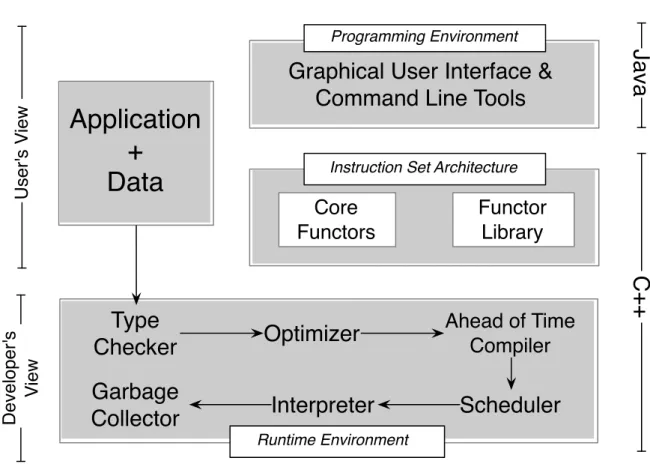
In this chapter we describe the new Dinamica EGO virtual machine and its core compo-nents. Dinamica EGO runs on top of a virtual machine called DinamicaVM. Figure 3.1 shows a schematic view of this virtual machine, including its programming environment. Dinamica provides its users with a Graphical User Interface, which is implemented in Java. It is also possible to load and run applications via a suite of command line tools. These applications are ensembles of functors. This virtual machine uses a set of func-tors, which includeApply,Reduce,Whileand Window. It also provides a suite of library components, which exist either due to efficiency reasons, or to keep compatibility with applications built prior to Dinamica 2.4.
The runtime environment of Dinamcia EGO consists of an optimizer, and ahead-of-time compiler, a scheduler, an interpreter and a garbage collector. The ahead-ahead-of-time compiler converts shading expressions, i.e., expressions that will be applied on every cell of a map or table, into binary code. These expressions are defined by Dinamica’s user through a syntax that we call EGO Script. Translation to binary works in two steps: first EGO Script commands are converted to C++ instructions. Then, these instructions are compiled into binary code by gcc. The scheduler sorts the functors
topologically, and forwards this information to the interpreter. If the target machine has multiple cores, then the scheduler parallelizes the execution of functors according to their dependences. The memory occupied by data structures that are no longer used are reclaimed by a garbage collector, which is based on reference counting. Cyclic dependences are not a problem in Dinamica, as it is not possible to create circular structures in it. In this section, we shall explore the four key components that this virtual machine interprets: Apply,Reduce,WindowandWhile. We also present a formal semantics model for EGO script.
20 Chapter 3. The Dinamica Virtual Machine
Graphical User Interface &
Command Line Tools
Functor
Library
Core
Functors
Optimizer
Garbage
Collector
Scheduler
Ahead of Time
Compiler
Runtime Environment
Interpreter
Instruction Set Architecture
Programming Environment
Ja
va
C
++
U se r' s V ie w D e ve lo p e r' s Vi e wType
Checker
Application
+
Data
Figure 3.1. A schematic view of Dinamica EGO’s Virtual Machine.
3.1
Apply
The Apply functor receives two inputs: (i) a map m, whose each cell has type t, e.g.,
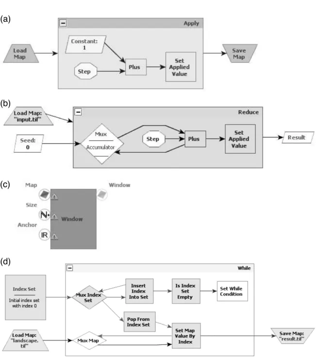
m : Maphti, and (ii) a function f : t 7→ t, that transforms the contents of each cell. The functor then applies f onto each cell of m, yielding a new map m′. Figure 3.2 (a) provides a visual representation of Apply when used in a program that increments every cell of a matrix of integers.
3.1. Apply 21
(a)
(b)
(c)
(d)
Figure 3.2. The four high-level functors in DinamicaVM’s instruction set archi-tecture. (a) Apply; (b)Reduce; (c)Window; (d)While.
elements, which come from contiguous positions in a column-major traversal of the map. The second internal port is Set, which causes a value to be written in a position of the output map that corresponds to the last index visited byStep in the input map. An Apply is used to obtain a map that is a function of another map. Examples of its use are:
22 Chapter 3. The Dinamica Virtual Machine
• Apply a normalization function producing a map where each cell is the result of a linear operation over the correspondent cell in the input map.
• Generate a map where each cell is replaced by the maximum adjacent neighbour.
Indeed, the applications are limitless and the programmer can use it to obtain great number of results.
Applyis one of the most used components in the Dinamica’s ecosystem. Examples of its use include mapping coordinates into administrative regions such as countries, states and municipalities; mapping altitude into costs; mapping cells into slope values, which are calculated given these cells’s neighbours, etc. Thus, it is very important that this component be implemented efficiently. Each iteration ofApplyuses data that is completely independent from the data used by the other iterations. In the PRAM (parallel random-access machine) model, Apply can be implemented to run in O(1). Thus, this functor is implemented to run in parallel.
3.2
Reduce
Reduce takes a map m of type Maphti, a binary operator ⊕, of type t′ ×t 7→ t′, and a seed s of type t′. It then produces a single value v of type t′, such that v =
s⊕m[0]⊕m[1]⊕. . .⊕m[n−1]. In this case, m[0], . . . m[n−1]are all the cells in m, assuming thatm has n cells. Figure 3.2 (b) shows an application that sums up all the elements in a map of integers, thus producing an integer as its result.
A user can utilize aReducein a variety of ways. The idea of theReduceoperation is to obtain a value that is a function of all values from a given input map. Therefore, this operator can be used, for instance, to obtain the maximum or minimum values from a map, to calculate the sum of all values or to retrieve the nearest point from a given coordinate.
Like Apply,Reduceis also aContainer. It has one internal input,Set, which bears the same semantics as the component of same name inApply. It has one internal output port,Step, which delivers to the internal functors the current value of the iteration. A functorMux performs the function of the accumulator used to keep track of the current value of a reduction. This functor, if applied on a n1×n2 map, runs sequentially in
3.3. Window 23
3.3
Window
Several applications implemented in Dinamica use small neighbourhoods within a map: finding the average slope of a coordinate, with regard to its neighbours; detecting bor-ders, smoothing images, applying convolutions, finding minimum/maximal cost paths, etc. Therefore, Dinamica provides users with an operator to find neighbourhoods in maps: the Windowfunctor, whose inputs and output are represented in Figure 3.2 (c).
Windowhas three inputs ports, which receive a map, the size of a neighbourhood’s side and an anchor, e.g., the coordinate that is the center of the neighbourhood. It outputs a set of cells that constitute the neighbourhood. Windows can be used to build filters along with the Apply and Reduce operators. Besides filters it is possible, e.g., to check for each cell of a given map if a certain feature is present in a defined neighbourhood or to produce a statistical analysis such as a kernel map. The vast majority of all the algorithms built in Dinamica use squared neighbourhoods whose sides contain an odd number of elements, and whose center point is the anchor. Because this setup is so common, it is heavily optimized, as we explain in Section 4.2.
3.4
While
Most of Dinamica EGO components are stateless. Data structures are usually copies, instead of being modified in place, for instance. However, there are cases when keeping track of state is desirable for efficiency reason. For instance, a stateless functor to model the movement of a ball, under the force of gravity only, when let loose onto an elevation map, could lead to a formidable number of copies of the target map. Dinamica avoids such situations by providing users with a statefull functor – the While iterator. The graphical representation of this element can be seen in Figure 3.2 (d).
An While has one input port, which receives an index set. An index set is a collection of sortable elements that index a data-structure: coordinates on a 2D or 3D map, points on a line, rows in a table, etc. The While has an internal Step port, which keeps track of the elements in the index set still to be processed. Whilealso has an internal Set port, which may update the index set with new elements. Thus, in practice, Whileimplements worklists: as long as the worklist is not empty, this functor perform an action. DinamicaVM uses While, for instance, to implement searches by depth and breadth in maps. A very common index set consists in contiguous sequences of integer numbers. This case is so common that we have a specialization of While – the Repeat functor – optimized to use it.
24 Chapter 3. The Dinamica Virtual Machine
map that is a function of an input map and a point within this map. An example would be to calculate a path for a road to be built given a cost map as input. Each iteration draws a new cell for the road that starts in a input point value and moves to the minimum neighbour in a 3x3 neighbourhood until a local minima is reached.
3.5
Specific Components
TheWhilefunctor seen in Section 3.4, plus the binary and unary operators of Dinamica EGO define a Turing complete language. Turing completeness comes from the fact that these functors subsume theWhileformalism, typically used to illustrate programming language semantics [Nielson and Nielson, 1992]. Nevertheless, there are applications that do not translate easily into amalgamations of these few elements. In particular, there exist behaviors that our optimizations from Section 4 do not derive automatically. Thus, Dinamica EGO provides a few specific – higher-level – components which are not implemented as combinations of the four previously described functors. These components are also necessary to keep compatibility with applications developed prior to Dinamica v2.4, which did not use the virtual machine that we describe here. In this section we describe one of these components as an example of a high-level operator.
For instance, Dinamica EGO contains a functor called CalcCostMap, which con-structs cost-surface maps out of raster images [Eastman, 1989]. The cost calculation problem is very common in land use simulations. The problem has two inputs: a fric-tion map, and a map of source points. The outcome of a cost calculafric-tion is a map that tells us, for each cell, the minimum cost to reach one of the source cells. This prob-lem emerges, for instance, whenever it is necessary to determine the paths that roads must traverse to link each interior city to a given set of harbours. The cost calculation problem is usually solved via chaotic iterations. We start with a solution map in which each cell is mapped to an infinitely large cost. Then, we iterate successive applications of the operator below, until a fixed point is reached:
y
cost(
x
) =
min
{
cost(
x
)
cost(
y
) + friction(
x
)
sqrt(2)
×
(cost(
z
) + friction(
x
))
z
z
x
y
y
y
z
z
3.5. Specific Components 25
(a) (b)
1 2 3 4
3 4 5 6
5 6 7 8
(c) (d)
Figure 3.3. (a) The four loops that implement the chaotic iterations of the
CalcCostMapfunctor. (b) Dependencies between tiles in the first loop: upper-left to lower-right. (c) Tiles with the same number can be processed together in the first loop. (d) Example of cost map that Dinamica produces.
independently. Figure 3.3(b) shows the pattern of dependences in the first loop, which traverses the map from the upper-left corner towards the lower-right corner. The execution runtime has a predefined number of available workers. Each worker has a task queue and can run a single task at a time. Tiles that must be processed are organized as a digraph of pending tasks. Tasks become eligible to run after all their dependencies have been processed. If a thread is idle, then it reclaims a tile that has no pending dependencies. This pattern continues until all the tiles have been processed. If the task queue of a processor becomes empty, then it might steal work from the queue of other processor. If a thread cannot steal any task, then it votes for the end of the computation. The computation terminates when a consensus is achieved among all the workers.
In this chapter we have presented our virtual machine and its components: Apply,
Chapter 4
Optimizations
In this chapter we present the optimizations implemented in the new DinamicaVM. These optimizations are divided in two groups: fusion optimizations and window opti-mizations. We also show the performace improvement through some case studies.
In order to be accepted by its users, the Dinamica Virtual Machine had to be at least as efficient as the original implementation of Dinamica’s runtime, which was used until Dinamica v2.4, last released in 2014. The key to achieve this efficiency are optimizations. Not only the implementations of Apply, Reduce, While and Window are highly engineered, but also the way that these components interact is optimized. All the optimizations that we describe here, except the prefetching from Section 4.2 1
, are applied after an application has been type checked, but before its modules start to run. EGO Script’s type system is static, i.e., types are known before an application starts running. Furthermore, this language does not support the dynamic loading of components, like PHP or JavaScript do. Therefore, we know the size of each map cell that is manipulated within an application, and we have a complete view of the dependence graph between components. This knowledge is important to generate code for the routines that read data, and move data between different functors. In this section we briefly touch the most important transformations that DinamicaVM applies onto its building blocks before an application runs. All the numbers that we show alongside the description of the optimization have been obtained in an Intel Core i5 with clock of 2.67GHz and 8GB of RAM.
1
Prefetching is part of the implementation ofWindow; it does not requires any program
transfor-mation.
28 Chapter 4. Optimizations
0.E+00% 2.E+03% 4.E+03% 6.E+03% 8.E+03% 1.E+04%
4500% 6000% 7500% 9000% 10500%
Split% Fused%
0.E+00% 2.E+03% 4.E+03% 6.E+03% 8.E+03% 1.E+04%
4500% 6000% 7500% 9000% 10500% Split% Fused%
Fusion of Div+Inc Fusion of Sum+Inc
Figure 4.1. Example of fusion. The Apply operator is always the increment
function, and the Reduceoperator is the sum of integers.
4.1
Fusion
Fusion is a transformation that we implement onto combinations ofApply+Apply, and
Apply+Reduce. This optimization is common in functional languages [Wadler, 1988]. It consists in combining the operators used by different functors in the following way:
Apply f (Apply g m) = Apply(f ◦g) m
Reduce s f (Apply g m) = Reduces f′ m wheref = λ(x, y). x⊕y
and f′ = λ(x, y). g(x)⊕y
Function fusion is not a new idea of ours. If fact, we are using a very limited form of fusion, as we only apply it to two combinations of functions. More extensive implementations have been described, for instance, by Jones et al. [Gill et al., 1993]. Nevertheless, our simple implementation of function fusion is enough to speed up some of Dinamica’s applications dramatically.
4.2. Window Optimizations 29
using three very simple instances of Apply and Reduce:
Inc m = Apply (λx . x+ 1) m
Div m = Apply (λx . x/2.17) m
Sum m = Reduce 0 (λ(x, y). x+y)m
In the figure we use random square matrixes of integers having sides of 5.0K, 7.5K and 10.0K cells. Without fusion DinamicaVM takes 9.940 seconds to Div◦Incevery cell of the 103
×103
matrix. Once fusion is activated, this time drops to 5.222 seconds. In the case of Reduce, gains are of similar nature. It takes us 7.294 seconds to Sum◦inc
the matrix with 10K rows without fusion, and 2.998 seconds if we use fusion. These gains are due to two factors: the elimination of intermediate data structures, and the improved locality. Concerning the first factor, fusion automatically eliminates the need to copy the map that the leftmost Apply produces. As for locality, the input map will be traversed only once instead of twice. Indeed, only one iteration is necessary for any sequence of applications of the Apply functor, e.g.:
applyf1 (. . .(apply fn m). . .) =apply (f1◦. . .◦fn) m
Fusion’s improvements are proportional to the complexity of the kernel operator used in Apply or Reduce. The more complex is the computation used inside these functors, less performance gains we shall observe. The composition below illustrates this trend:
Apply Normalize (apply calcSlope m)
Normalizeis a simple linear function of the input value, but thecalcSlopeoperation is a substantially more complex functor present in the Dinamica EGO library. It applies a
Reduceover the output of aWindowfor each index in the input map. For a7500×7500 input map, fusion gives us 6% of speedup in this example.
4.2
Window Optimizations
30 Chapter 4. Optimizations
(c) • • •
• • •
(a) (b)
Line 1
Line 2
Line 3
Figure 4.2. The three-lines cache. The dashed arrows show line pointers in the
previous iteration of Window. The solid arrows show the pointers in the current
iteration. (a) Input map. (b) Cached lines. (c) Center of 3×3window.
4.2.1
Prefetching
Most of the applications that use Window slide it over an image in row-major order, that is, starting from the upper-left corner of an image, and going to its lower-right corner. This pattern is so common because it is the default order in whichApply and
Reduce evaluate the elements of a map. Our optimizer ensures that each cell of a
Windowis read only once from main memory, ifWindowis used in that way. To ensure this property, we pre-fetch the lines that will be traversed byWindow.
Figure 4.2 illustrates this approach for a3×3instance ofWindow. In this example, each timeWindowis called, it reads nine elements of the input map. Instead of fetching this data when Window is created, we pre-fetch three entire lines of the map, and let
Window slide on these lines. OnceWindow reaches the rightmost border of the image, we discard the topmost line, and read one line more from main memory. If Window
works with submatrices of n rows, then we should, in principle, keep n lines in cache. However, most of the applications available in the Dinamica’s ecosystem work with 3×3windows. Thus, we chose to work with only three lines at a time. Consequently, larger instances of Windowmay lead to multiple trips to the main memory.
The prefetching is only necessary for maps that cannot fit entirely in the L0 cache. This is usually the case in Dinamica, as maps are very large, and each of their cells contains a non-negligible amount of data, which include colour patterns and geographic information. In the absence of this optimization, a n ×n Window causes each – non-border – map cell to be read n2
times. Usually data in the same row of
4.2. Window Optimizations 31
0 1000 2000 3000 4000 5000 6000
0 5 10 15 20 25 30 35 40
Dinamica 2.4 DVM -‐ No Opt DVM -‐ Prefetching
Figure 4.3. Performance gain due to prefetching in an image smoother.
4.2.2
Performance Improvement due to Pre-fetching
Figure 4.3 shows the performance of three different instances of an image smoothing algorithm. The algorithm uses a 3×3 convolution matrix that does simple average to implement smoothing. The smoothing filter returns, for a given cell i, the average of all the immediate neighbours of i plus i itself. The three instances of the algorithm are:
• Library – the algorithm was implemented using a monolithic smoothing filter available in Dinamica’s library.
• DVM - No Opt– our algorithm, built as the following combination of functors:
Smooth m =Apply ((Reduce Average)◦Window) m
• DVM - Prefetching – the previous implementation, with prefetching enabled in DinamicaVM.
32 Chapter 4. Optimizations
0 2000 4000 6000 8000 10000 12000 14000
4 6 8 10 12 14 16 EGO v2.4 VM Base Prefetch Prefetch & Unroll
Figure 4.4. Performance gains in Conway’s Game of Life (Section 1.1) due to unrolling and prefetching. X-axis is the number of generations of the automaton, and Y-axis is runtime, in msecs.
4.2.3
Unrolling
The most used type of Window is a 3× 3 squared view of a map, with anchor in the center. Because this pattern is so common, we use a special implementation of it, which has no control flow. This implementation reads a chunk of memory that is large enough to fit each one of the nine indices to be processed. It then divides this memory into nine pieces, and fills up the positions in the map view with them. The size of memory that must be read is determined by the ahead-of-time compiler, before
Windowis invoked, but after the type of its input is already known.
4.2. Window Optimizations 33
us 57% faster than the old version of Dinamica. In other words, the two optimizations makes our virtual machine 3.6x faster.
The set of optimizations presented in this chapter are twofold: fusion and window optimizations. The former acts over sequences of operatorsApplyor sequences ofApply
Chapter 5
A Semantics Model of EGO Script
and the Copy Elimination
Optimization
In this chapter we describe a core optimization we have implemented in the Dinamica EGO evironment. This optimization eliminate data copies and allows the execution environment to overwrite data structures while keeping referential transparency that is a key feature in the language. To present this optimization we first define a formal semantics model for the EGO Script language. After, we present the copy elimination algorithm and two case studies to show the arising performance improvement.
In order to provide users with a high-level programming environment, one of the key aspects of Dinamica’s semantics is referential transparency. This is a feature frequently found in dataflow programming languages [Johnston et al., 2004] The com-ponents in a Dinamica EGO script must not modify the data that they receive as inputs. A typical way to ensure referential transparency is to rely on immutable data structures [Sondergaard and Sestoft, 1990]. If the contents of a data structure must be updated, then the whole data is copied into a new memory location. However, this alternative is too expensive in Dinamica, because our data structures – maps and tables – tend to be very large. Therefore, a copy minimization algorithm is essential to allow these applications to scale. Removing these copies is a non-trivial endeavor, inasmuch as minimizing such copies is a NP-complete problem, as we show in Section 5.2.
We demonstrate the effectiveness of our optimization via two case studies. The first one divides an altitude map into slices of same height. In order to get more precise ground information, we must decrease the height of each slice; hence, increasing the amount of slices in the overall database. In this case, for highly accurate simulations
36
Chapter 5. A Semantics Model of EGO Script and the Copy Elimination Optimization mux map slopes map cities Table T Empty Group 1 Calculate mean slope
for one city W1 T[x] ← mean slope of city x
R1 Get total number of cities
W3 Set number of cities at T[-1]
W2
Set mean slope of the whole map at T[-2]
Table T -2: mean slope -1: N i, 0 < i < N: mean slope of each city Categories
For each category (for each city)
R2 Get mean slot of all the cities T T T|| T|| T|| T T T Lp
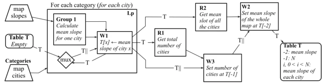
Figure 5.1. An EGO Script program that finds the average slope of the cities that form a certain region. The parallel bars denote places where the original implementation of Dinamica EGO replicates data.
our copy elimination algorithm boosts the performance of Dinamica EGO by almost 100x. The second model - simpler - performs an statistical analysis of map values getting data such as sum of values, variance and standard deviation.
5.1
Dinamica EGO in Another Example
As we did in Section 1.1 we present here another application implemented in Dinamica EGO. This example will guide us to state the copy minimization algorithm in Sec-tion 5.4. Although simple, this applicaSec-tion contains some of the key elements that we will discuss in the rest of this chapter. More examples can be found in the Dinamica EGO Guidebook1
.
Consider the following problem: “what is the mean slope of the cities from a given region?” We can answer this query by combining data from two maps encompassing the same geographic area. The first map contains the slope of each area. We can assume that each cell of this matrix represents a region of a few hectares, and that the value stored in it is the average slope of that region. The second map is a matrix that associates with each region a number that identifies the municipality where that region is located. Regions that are part of the same city jurisdiction have the same identifier. The EGO script that solves this problem is shown in Figure 5.1. An EGO Script program is an ensemble of components, which are linked together by data channels. Some components encode data, others computation. Components in this last category are called functors. The order in which functors must execute is determined by the runtime environment, and should obey the dependencies created by the data channels.
1