DATA CHARACTERIZATION TOWARDS MODELING FREQUENT PATTERN MINING ALGORITHMS

Natarajan Meghanathan et al. (Eds) : WiMONe, NCS, SPM, CSEIT - 2014

pp. 285–304, 2014. © CS & IT-CSCP 2014 DOI : 10.5121/csit.2014.41223

Sayaka Akioka

School of Interdisciplinary Mathematical Sciences, Meiji University, Tokyo, Japan

akioka@meiji.ac.jp

ABSTRACT

Big data quickly comes under the spotlight in recent years. As big data is supposed to handle extremely huge amount of data, it is quite natural that the demand for the computational environment to accelerates, and scales out big data applications increases. The important thing is, however, the behavior of big data applications is not clearly defined yet. Among big data applications, this paper specifically focuses on stream mining applications. The behavior of stream mining applications varies according to the characteristics of the input data. The parameters for data characterization are, however, not clearly defined yet, and there is no study investigating explicit relationships between the input data, and stream mining applications, either. Therefore, this paper picks up frequent pattern mining as one of the representative stream mining applications, and interprets the relationships between the characteristics of the input data, and behaviors of signature algorithms for frequent pattern mining.

KEYWORDS

Stream Mining, Frequent Mining, Characterization, Modeling, Task Graph

1. INTRODUCTION

Big data quickly comes under the spotlight in recent years. Big data is expected to collect gigantic amount of data from various data sources, and analyze those data across conventional problem domains in order to uncover new findings, or people's needs. As big data is supposed to handle extremely huge amount of data compared to the conventional applications, it is quite natural that the demand for the computational environment, which accelerates, and scales out big data applications, increases. The important thing here is, however, the behavior or characteristics of big data applications are not clearly defined yet.

High performance computing community has been investigating data intensive applications, which analyze huge amount of data as well. Raicu et al. pointed out that data intensive applications, and stream mining applications are fundamentally different from the viewpoint of data access patterns, and therefore the strategies for speed-up of data intensive applications, and stream mining applications have to be radically different [32]. Many data intensive applications often reuse input data, and the primary strategy of the speed-up is locating the data close to the target CPUs. Stream mining applications, however, rarely reuse input data, so this strategy for data intensive applications does not work in many cases. Modern computational environment has been and is evolving mainly for speed-up of benchmarks such as Linpack [33], or SPEC [34]. These benchmarks are relatively scalable according to the number of CPUs. Stream mining applications are not scalable to the contrary, and the current computational environment is not necessarily ideal for stream mining applications. The simplest approach is to use this template and insert headings and text into it as appropriate. Additionally, many researchers from machine learning domain, or data mining domain point out that the behavior, execution time more specifically, of stream mining applications varies according to the characteristics, or features of the input data. The problem is, however, the parameters, or the methodology for data characterization is not clearly defined yet, and there is no study investigating explicit relationships between the characteristics of the input data, and the behavior of stream mining applications, either.

Therefore, this paper picks up frequent pattern mining as one of the representative stream mining applications, and interprets the relationships between the characteristics of the input data, and behaviors of signature algorithms for frequent pattern mining. The rest of this paper is organized as follows. Section 2 describes a model of stream mining algorithms in order to share the awareness of the problem, which this paper focuses on. Then, the section also briefly introduces related work. Section 3 overviews the application that this paper picks up, and illustrates the algorithms those are typical solutions for the application. Section 4 explains the methodology of the experiments, shows the results, and gives discussions over those results. Section 5 concludes this paper.

2. R

W

2.1. A Model of Stream Mining Algorithms

A stream mining algorithm is an algorithm specialized for a data analysis over data streams on the fly. There are many variations of stream mining algorithms, however, general stream mining algorithms share a fundamental structure, and a data access pattern as shown in Figure 1 [35]. A stream mining algorithm consists of two parts, stream processing part, and query processing part. First, the stream processing module in stream processing part picks the target data unit, which is a chunk of data arrived in a limited time frame, and executes a quick analysis over the data unit. The quick analysis can be a preconditioning process such as a morphological analysis, or a word counting. Second, the stream processing module in stream processing part updates the data, which are cached in one or more sketches, with the latest results through the quick analysis. That is, the sketches keep the intermediate analysis, and the stream processing module updates the analysis incrementally as more data units are processed. Third, the analysis module in stream processing part reads the intermediate analysis from the sketches, and extracts the essence of the data in order to complete the quick analysis in the stream processing part. Finally, the query processing part receives this essence for the further analysis, and the whole process for the target data unit is completed.

processing part has the huge impact over the latency of the whole process. The stream processing part also needs to finish the preconditioning of the current data unit before the next data unit arrives. Otherwise, the next data unit will be lost as there is no storage for buffering the incoming data in a stream mining algorithm. On the other hand, the query processing part takes care of the detailed analysis such as a frequent pattern analysis, or a hot topic extraction based on the

Figure 1. A model of stream mining algorithms.

intermediate data passed by the stream processing part. The output by the query processing part is usually pushed into a database system, and there is no such an urgent demand for an instantaneous response. Therefore, only the stream processing part needs to run on a real-time basis, and the successful analysis over all the incoming data simply relies on the speed of the stream processing part.

The model in Figure 1 also indicates that the data access pattern of the stream mining algorithms is totally different from the data access pattern of so-called data intensive applications, which is intensively investigated in high performance computing community. The data access pattern in the data intensive applications is a write-once-read-many [32]. That is, the application refers to the necessary data repeatedly during the computation. Therefore, the key for the speedup of the application is to place the necessary data close to the computational nodes for the faster data accesses throughout the execution of the target application. On the other hand, in a stream mining algorithm, a process refers to its data unit only once, which is a read-once-write-once style. Therefore, a scheduling algorithm for the data intensive applications is not simply applicable for the purpose of the speedup of a stream mining algorithm.

of these dependencies are essential to keep the analysis results consistent, and correct. The three data dependencies are as follows, and the control flow for the correct execution generates all these data dependencies.

Figure 2. Data dependencies of the stream processing part in two processes in line.

• The processing module in the preceding process should finish updating the sketches before the processing module in the successive process starts reading the sketches (Dep.1 in Figure 2).

• The processing module should finish updating the sketches before the analysis module in

the same process starts reading the sketches (Dep. 2 in Figure 2).

• The analysis module in the preceding process should finish reading the sketches before

the processing module in the successive process starts updating the sketches (Dep. 3 in Figure 2).

2.2. A Task Graph

A task graph is a kind of pattern diagrams, which represents data dependencies, control flows, and computational costs regarding a target implementation. A task graph is quite popular for scheduling algorithm researchers. In the process of the development of scheduling algorithms, the task graph of the target implementation works as if a benchmark, and provides the way to develop a scheduling algorithm in a reproducible fashion. The actual execution of the target implementation in the actual computational environment provides realistic measurement, however, the measurement varies according to the conditions such as computational load, or timings at the moment. This fact makes difficult to compare different scheduling algorithms in order to determine which scheduling algorithm is the best for the target implementation with the target computational environment. A task graph solves this problem, and enables fair comparison of scheduling algorithms through simulations.

for all training data do (1) fetch one data unit for all attributes for do

(2-1) update the weight sum for this attribute (2-2) update the mean value of this attribute end for

end for

Figure 4 algorithm.

As discussed in the previous section, the model of a stream mining algorithm has data dependencies both across the processes, and inside one process. Therefore, a task graph for a stream mining algorithm should consist of a data dependency graph, and a control flow graph [36]. Figure 3 is an example of a task graph of the training stage of Naïve Bayes classifier [37]. In Figure 3, the left figure is a data dependency graph, and the right figure is a control flow graph. Figure 4 represents the pseudo code for the task graph shown in Figure 3.

Both a data dependency graph, and a control flow graph are directed acyclic graphs (DAGs).In a task graph, each node represents a meaningful part of the input code. Nodes in white are codes in the preceding process, and nodes in gray are codes in the successive process.The nodes with the same number represents the same meaningful part in the input source code, and the corresponding line in the pseudo code shown in Figure 4. The nodes with the same number in the same color indicate that the particular part of the input source code is runnable in parallel. Here, nodes in a control flow graph have numbers. Each number represents execution cost of the corresponding node. Each array in a data dependency graph indicates a data dependency. If an arrow comes up from node A to node B, the arrow indicates that node B relies on the data generated by node A. Similarly, each array in a control flow graph represents the order of the execution between nodes. If an arrow comes up from node A to node B, the arrow indicates that node A has to be finished before node B starts. The nodes in the same level are possible to be executed in parallel.The nodes with the same number indicate that the particular line in the pseudo code is runnable in parallel. There are two major difficulties for describing stream mining applications with task graphs. One problem is that the concrete parallelism strongly relies on the characteristics of the input data. The other problem is that a cost for a node varies according to the input data. That is, a task graph for a stream mining application is impossible without the input data modeling.

2.3. Related Work

There are several studies on task graph generation, mainly focusing on generation of random task graphs. A few projects reported task graphs generated based on the actual well-known applications; however, those applications are from numerical applications such as Fast Fourier Transformation, or other applications familiar to high performance computing community for years.

Task Graphs for Free (TGFF) provides pseudo-random task graphs [38, 39]. TGFF allows users to control several parameters, however, generates only directed acyclic graphs (DAGs) with one or multiple start nodes, and one or multiple sink nodes. A period, and deadline is assigned to each task graph based on the length of the maximum path in the graph, and the user specified parameters.

task graphs, based on the longest path, the distribution of the out-degree, and the number of edges.

Task graph generator provides both random task graphs, and task graphs extracted from the actual implementations such as Fast Fourier Transformation, Gaussian Elimination, and LU Decomposition [41]. Task graph generator also provides a random task graph generator which supports a variety of network topologies including star, and ring. Task graph generator also provides scheduling algorithms as well.

Tobita et al. proposed Standard Task Graph Set (STG), evaluated several scheduling algorithms, and published the optimal schedules for STG [42, 43]. STG is basically a set of random task graphs. Tobita et al. also provided task graphs from numerical applications such as a robot control programs, a sparse matrix solver, and SPEC fpppp [34].

Besides the studies on task graph generation, Cordeiro et al. pointed out that randomly generated task graphs can create biased scheduling results, and that the biased results can mislead the analysis of scheduling algorithms [40]. According to the experiments by Cordeiro et al., a same scheduling algorithm can obtain a speedup of 3.5 times for the performance evaluation only by changing the random graph generation algorithm. Random task graphs contribute for evaluation of scheduling algorithms, however, do not perfectly cover all the domains of parallel, and distributed applications as Cordeiro et al. figured out in their work. Especially for stream mining applications, which this paper focuses on, the characteristic of the application behaviors is quite different from the characteristic of the applications familiar to the conventional high performance computing community [32]. Task graphs generated from the actual stream mining applications have profound significance in the better optimization of stream mining applications.

These all projects point out the importance of fair task graphs, and seek the best solution for this problem. These projects, however, focus only on data dependencies, control flows, and computational costs of each piece of an implementation. The computational costs are often decided in a random manner, or based on the measurements through speculative executions. No project pays attention to the relationships between the variation of the computational costs, and the characteristics of the input data.

3. ALGORITHMS

3.1. Frequent Pattern Mining

This paper focuses on two algorithms for frequent pattern mining. Frequent pattern mining was originally introduced by Agrawal et al. [44], and the baseline is the mining over the stores items purchased on a per-transaction-basis. The goal of the mining is finding out all the association rules between sets of items with some minimum specified confidence. One of the examples of the association rules is that 90% of transactions purchasing bread, and butter purchase milk as well. That is, the association rules those appearances are greater than the specified confidence are regarded as frequent patterns. Here, in the rest of this paper, the confidence is called "(minimum) support".

3.2. Apriori

Figure5 gives Apriori algorithm, and there are several assumptions as follows. The items in each transaction are sorted in alphabetical order. We call the number of items in an itemset its “size”, and call an itemset of size a - .Items in an itemset are in alphabetical order again. We call an itemset with minimum support a "large itemset".

Figure 5. The pseudo-code for Apriori algorithm.

Figure 6. The pseudo-code for the join step of apriorigen function.

Figure 7. The pseudo-code for the prune step of apriorigen function.

The first pass of Apriori algorithm counts item occurrences in order to determine the 1 (line (1) in Figure 5). A subsequent pass consists of two phases. Suppose we are in

-ℎ pass. First, the found in the ( − 1)- ℎ pass are used for generating the candidate itemsets (potentially large itemsets), using the function, which we describe later in this section (line (2) in Figure 5). Next, the database is scanned, and the support of candidates in is counted (line (3) and (4) in Figure 5). These two phrases prepare for the (line (5) in Figure 5), and the subsequent pass is repeated until becomes empty.The function takes , and returns a superset of the set of all the

The distinctive part of Apriori algorithm is the function. The function reduces the size of candidate sets, and this reduction contributes for speed-up of the mining. The function is designed based on Apriori heuristic [45]; if any length pattern is not frequent in the database, its length + 1 super-pattern can never be frequent.

3.3. FP-growth

FP-growth algorithm is proposed by Han et al. [46], and they point out Apriori algorithm suffers from the cost for handling huge candidate sets, or repeated scanning database with prolific frequent patterns, long patterns, or quite low minimum support. Han et al. advocated the bottleneck exists in candidate set generation, and test, and proposed frequent pattern tree (FP-tree) as one of the alternatives.Here, we see the construction process of FP-tree, utilizing the example shown on Table 1. In this example, we set the minimum support as "three times", instead of appearance ratio in order to simplify the explanation. The FP-tree developed from this example is shown in Figure 8.

Table 1. The input example for FP-growth algorithm.

TID item series frequent items (for reference) 100 f, a, c, d, g, i, m, p f, c, a, m, p

200 a, b, c, f, l, m, o f, c, a, b, m

300 b, f, h, j, o f, b

400 b, c, k, s, p c, b, p

500 a, f, c, e, l, p, m, n f, c, a, m, p

First, the first data scan is conducted for generating the list of frequent items. The obtained list looks like as follows.

< (f: 4), (c: 4), (a: 3), (b: 3), (m: 3), (p: 3) >

Here, (&: ()represents item&appears ( times in the database. Notice the list is ordered in frequency descending order. The ordering is important as each path of a tree follows this ordering. The rightmost column on Table 1 represets the frequent items in each transaction.

Next, we start generating a tree with putting the root of a tree, labeled with "null". The second data scan is conducted for generating the FP-tree. The scan of the first transaction constructs the first branch of the tree:

< (f: 1), (c: 1), (a: 1), (m: 1), (p: 1) >

Again, notice the frequent items in the transaction are ordered in the same order to the list of frequent items. For the second transaction, its frequent item list < ), (, , *, > shares a common prefix < ), (, > with the existing path < ), (, , , >, we simply increment the counts of the common prefix, and create a new node (b: 1) as a child of (a: 2). Another new node

(m: 1) is created as a child of (b: 1). For the third transaction, its frequent item list < ), * >

introduces a completely new branch as follows, because no node is shared with existing prefix trees.

< ((: 1), (*: 1), ( : 1) >

Figure 8. An example of FP-tree.Figure 4. A pseudo code for the training stage of Naïve Bayes

The frequent items in thelast transaction perfectly overlaps with the frequent items in the first transaction. Therefore, we simply increment the counts in the path< ), (, , , >.Figure 8 is a complete FP-tree developed from this example. In the left part of Figure 8, there is an item header table, and this table contains head of node-links. This header table is utilized for tree traversal when extracting all the frequent patterns.

4. EXPERIMENTS

4.1. Setup

The purpose of this paper is to interpret the relationships between the characteristics of the input data, and behaviors of frequent pattern mining algorithms such as Apriori algorithm, and FP-growth algorithm. This section explains the methodology for the experiment for collecting data for the investigation.

We utilize the implementations of Apriori algorithm [47], and FP-growth algorithm [48] in C, which are distributed by Borgelt. We compiled, and run the programs as they are for fairness. No optimization is applied. In order to observe changes of the behaviors of these programs, three kinds of data are prepared as input. The overall feature of each data is summarized as Table 2. The details of each data are as follows.

Table 2. Summary of the input data.

number of transactions number of distinct items

census 48,842 135

papertitle 2,104,240 925,151

• census: This is national population census data, and the data are distributed with Apriori

algorithm implementation [47], and FP-growth implementation [48] by Borgelt as test data. A couple of lines from the actual data as an example are shown in Figure 9. As shown on Table 2, the ratio of the number of distinct items to the number of transactions is moderate among the three input data, and the ratio is 0.28%. We also see the number of transactions in census is the smallest.

• papertitle: This is the data set for KDD Cup 2013 Author-Paper Identification Challenge

(Track 1), and available at Kaggle contest site [49]. We extract paper titles from Paper.csv, and create the list of titles for the experiments here. A couple of lines from the actual data as an example are shown in Figure 10. As shown on Table 2, the ratio of the number of distinct items to the number of transactions is extremely high compared to the other two data sets, and the ratio is 44.0%. We also see the number of transactions is moderately high.

Figure 9. Examples of census.

Figure 10. Examples of papertitle.

Figure 11. Examples of shoppers.

• shoppers: This is the data set for Acquire Valued Shoppers Challenge, and available at

From the viewpoint of the application, the meaning of frequent mining over census is finding out typical portraits of the nation. Similarly, frequent mining over papertitle derives popular sets of words (not phrases) in paper titles, and frequent mining over shoppers extracts frequent combinations of item categories in the purchased items.

4.2. Results

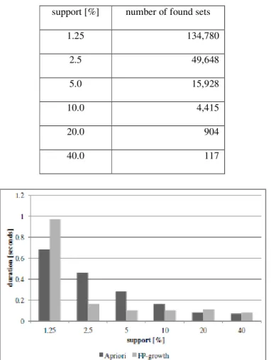
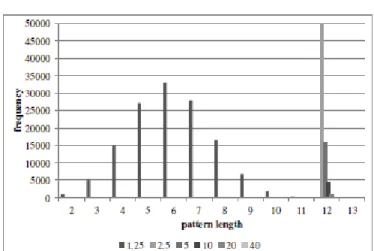
Table 3 shows the number of found sets for census when support increases from 1.25 to 40. Both Apriori algorithm, and FP-growth algorithm found the same number of sets for the same support. Figure 12 compares the execution times in seconds of Apriori algorithm, and FP-growth algorithm for each support. Figure 13 shows the details of the execution times of Apriori algorithm for each support. Similarly, Figure 14 shows the details of the execution times of FP-growth algorithm for each support. Figure 15 shows the frequency graph of the found pattern length for each support. Here, both algorithms found the same patterns; the frequency shown in this graph is common to both Apriori algorithm, and FP-growth algorithm.

Table 3. Number of found sets (census). support [%] number of found sets

1.25 134,780

2.5 49,648

5.0 15,928

10.0 4,415

20.0 904

40.0 117

Figure 13. Details of Apriori (census).

Although the number of transactions is moderate among the three cases, the number of the found sets is quite huge compared to the other two cases (we see later on Table 4, and Table 5). This is reasonable as the ratio of the number of distinct items to the number of transactions in the input data is quite small (Table 2). According to [46], Apriori algorithm is expected to be behind because of the large number of frequent sets, and the quite low support. Figure 12 shows, however, FP-growth algorithm overcomes Apriori algorithm only when support is 2.5%, 5%, and 10%. The case with 1.25% support is supposed to be the worst case for Apriori algorithm for its low support, and the huge number of frequent sets; however, Apriori algorithm is faster than FP-growth algorithm. The details of the execution times of the two algorithms suggest the explanation of this situation. As shown in Figure 13, Apriori algorithm increases its execution time of the main part of the algorithm gently, and the curve matches to the decrease of the support. The cost for the writing part is almost constant regardless of the support contrary. Figure 14 shows FP-growth algorithm suffers from sudden and drastic increase in sorting-reducing transactions part, and writing part, and this increase caused the behind. As both Apriori algorithm, and FP-growth algorithm output the same number of sets, the sudden increase in the writing part of FP-growth algorithm apparently implicates the overhead exists in the implementation for this case. According to Han et al., Apriori algorithm suffers from the longer frequent pattern [46]. Figure 15 shows that the length of the found set is mostly centering around 12, however, scattered from 2 to 10 in the case with support value of 1.25. This tendency also indicates that the lower support value allowed the shorter pattern more, and this situation may helped Apriori algorithm, and contributed to the better performance of Apriori algorithm even with the smaller support value.

Figure 14. Details of FP-growth (census).

Figure 15. Pattern length (census). Table 4. Number of found sets (papertitle).

support [%] number of found sets

1.25 49

2.5 21

5.0 8

10.0 3

20.0 0

40.0 0

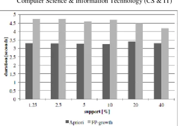
Figure 16. Comparison of durations between Apriori and FP-growth (papertitle).

Figure 17. Details of Apriori (papertitle).

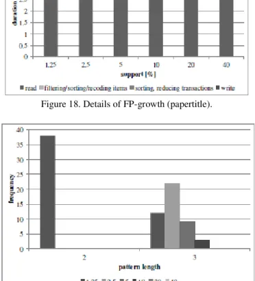
Considering the characteristics of Apriori algorithm, and FP-growth algorithm, Apriori algorithm is expected to be of advantage. Actually, Figure 16 shows Apriori algorithm is always faster than FP-growth algorithm regardless of support. Figure 17 shows Apriori algorithm does not spend meaningful time for the main part of the algorithm. Figure 18 shows FP-growth algorithm spends a certain time on the main part of the algorithm, and the impact on the overall execution time remains almost on the same level. There is no drastic increase in both writing part, and the main body of the algorithm; however, this is because the number of the found sets stays small even with the smallest support. Figure 19 shows the length of the found pattern is 2 or 3 in all the cases, which is very short, and supports the results that Apriori algorithm outperformed FP-growth algorithm.

the ratio of the number of distinct items to the number of transactions is extremely small as shown on Table 5. Based on the observation of the characteristics of the input data, the number of the found sets shown in Table 5 indicates the ratio of the number of distinct items to the number of transactions is not necessarily perfect as the measure of the number of frequent sets. This is not surprising, of course, and we need to introduce some other parameters such as distribution to preconjecture the number of frequent sets from the input data. With the number of the found sets is moderately small; Apriori algorithm is always faster than FP-growth algorithm regardless of support again. Different from papertitle, however, both Apriori algorithm and FP-growth algorithm increase execution times as support decreases. One more thing to be considered is that Apriori algorithm increases the execution time in the main part of the algorithm as support decreases (Figure 21), however, FP-growth algorithm spends more time in reading as support decreases (Figure 22). Figure 23 also shows the length of the found sets is relatively small, which is from 2 to 4, and the situation is favorable for Apriori algorithm. This result also supports why Apriori algorithm outperformed FP-growth algorithm.

Figure 18. Details of FP-growth (papertitle).

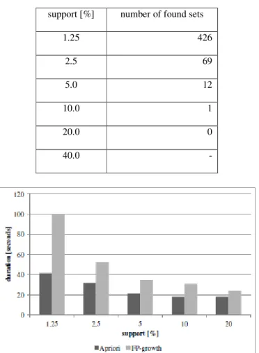
Table 5. Number of found sets (shoppers). support [%] number of found sets

1.25 426

2.5 69

5.0 12

10.0 1

20.0 0

40.0 -

Figure 20. Comparison of durations between Apriori and FP-growth (shoppers). 4.3. Discussion

The overall results clearly indicate that simple one measure such as the total number of transactions, or the total number of distinct items does not contribute for algorithm selection. Actually, Apriori algorithm is considered to be hard to scale, however, Apriori algorithm was faster than FP-growth algorithm in papertitle case, and shoppers case, even though these two cases handle huge number of transactions compared to census case. Apparently, the characteristics of the input data should be determined in order to select appropriate algorithm.

Figure 21. Details of Apriori (shoppers).

Figure 22. Details of FP-growth (shoppers).

Figure 23. Pattern length (shoppers).

writing data, and that FP-tree has a close relation to the increase of the execution time for these two parts.

5. CONCLUSIONS

Big data quickly comes under the spotlight in recent years, and increases its importance both in socially, and scientifically. Among big data applications, this paper specifically focused on frequent mining, and gave the first step to interpret the relationships between the characteristics of the input data, and behaviors of signature algorithms for frequent pattern mining. The experiments, and discussions backed up that the characteristics of the input data have certain impact on both the performance, and the selection of the algorithm to be utilized. This paper also picked up some parameters for characterizing the input data, and showed these parameters are meaningful, however, revealed some items to be investigated for the better characterization of the input data as well.

REFERENCES

[1] B. Babcock, M. Datar, R. Motwani, and L. O’Callaghan, “Maintaining variance and k-medians over data stream windows,” in Proceedings of the Twenty-second ACM SIGMOD-SIGACT-SIGART Symposium on Principles of Database Systems, ser. PODS ’03. New York, NY, USA: ACM, 2003, pp. 234–243.

[2] N. Tatbul, U. C¸ etintemel, S. Zdonik, M. Cherniack, and M. Stonebraker,“ Load shedding in a data stream manager,” in Proceedings of the29th International Conference on Very Large Data Bases - Volume 29,ser. VLDB ’03. VLDB Endowment, 2003, pp. 309–320.

[3] B. Babcock, S. Babu, M. Datar, R. Motwani, and J. Widom, “Models and issues in data stream systems,” in Proceedings of the Twenty-first ACM SIGMOD-SIGACT-SIGART Symposium on Principles of Database Systems, ser. PODS ’02. New York, NY, USA: ACM, 2002, pp.1–16.

[4] A. C. Gilbert, Y. Kotidis, S. Muthukrishnan, and M. Strauss, “Surfing wavelets on streams: One-pass summaries for approximate aggregate queries,” in Proceedings of the 27th International Conference on VeryLarge Data Bases, ser. VLDB ’01. San Francisco, CA, USA: Morgan Kaufmann Publishers Inc., 2001, pp. 79–88.

[5] C. C. Aggarwal, J. Han, J. Wang, and P. S. Yu, “A framework for clustering evolving data streams,” in Proceedings of the 29thInternational Conference on Very Large Data Bases - Volume 29, ser. VLDB ’03. VLDB Endowment, 2003, pp. 81–92.

[6] C. C. Aggarwal, J. Han, J. Wang, and P. S. Yu, “A framework for projected clustering of high dimensional datastreams,” in Proceedings of the Thirtieth International Conference on Very Large Data Bases - Volume 30, ser. VLDB ’04.VLDB Endowment, 2004, pp. 852–863.

[7] C. C. Aggarwal, J. Han, J. Wang, and P. S. Yu, “On demand classification of data streams,” in Proceedings of the Tenth ACM SIGKDD International Conference on Knowledge Discovery and Data Mining, ser. KDD ’04. New York, NY, USA:ACM, 2004, pp. 503–508.

[8] G. Cormode and S. Muthukrishnan, “What’s hot and what’s not: Tracking most frequent items dynamically,” ACM Trans. Database Syst., vol. 30, no. 1, pp. 249–278, Mar. 2005.

[9] G. Dong, J. Han, L. V. S. Lakshmanan, J. Pei, H. Wang, and P. S. Yu, “Online mining of changes from data streams: Research problems and preliminary results,” in Proceedings of the 2003 ACM SIGMOD Workshop on Management and Processing of Data Streams. In cooperation with the 2003 ACM-SIGMOD International Conference on Management of Data, 2003.

[10] S. Guha, A. Meyerson, N. Mishra, R. Motwani, and L. O’Callaghan,“Clustering data streams: Theory and practice,” IEEE Trans. on Knowl.and Data Eng., vol. 15, no. 3, pp. 515–528, Mar. 2003.

[11] M. Charikar, L. O’Callaghan, and R. Panigrahy, “Better streaming algorithms for clustering problems,” in Proceedings of the Thirty-fifth Annual ACM Symposium on Theory of Computing, ser. STOC ’03.New York, NY, USA: ACM, 2003, pp. 30–39. [Online].

[13] G. Hulten, L. Spencer, and P. Domingos, “Mining time-changing datastreams,” in Proceedings of the Seventh ACM SIGKDD International Conference on Knowledge Discovery and Data Mining, ser. KDD ’01.New York, NY, USA: ACM, 2001, pp. 97–106.

[14] L. O’Callaghan, N. Mishra, A. Meyerson, S. Guha, and R. Motwani,“Streaming-data algorithms for high-quality clustering,” in Proceedings of the 18th International Conference on Data Engineering, ser. ICDE’02. Washington, DC, USA: IEEE Computer Society, 2002, pp. 685–.

[15] C. Ordonez, “Clustering binary data streams with k-means,” in Proceedings of the 8th ACM SIGMOD Workshop on Research Issues in Data Mining and Knowledge Discovery, ser. DMKD ’03.New York, NY, USA: ACM, 2003, pp. 12–19.

[16] E. Keogh and J. Lin, “Clustering of time-series subsequences is meaningless: Implications for previous and future research,” Knowl.Inf. Syst., vol. 8, no. 2, pp. 154–177, Aug. 2005.

[17] H. Wang, W. Fan, P. S. Yu, and J. Han, “Mining concept-drifting datastreams using ensemble classifiers,” in Proceedings of the Ninth ACMSIGKDD International Conference on Knowledge Discovery and DataMining, ser. KDD ’03. New York, NY, USA: ACM, 2003, pp. 226–235.

[18] V. Ganti, J. Gehrke, and R. Ramakrishnan, “Mining data streams under block evolution,” SIGKDD Explor. Newsl., vol. 3, no. 2, pp. 1–10, Jan.2002.

[19] S. Papadimitriou, A. Brockwell, and C. Faloutsos, “Adaptive,hands-off stream mining,” in Proceedings of the 29th International Conference on Very Large Data Bases - Volume 29, ser. VLDB’03. VLDB Endowment, 2003, pp. 560–571.

[20] M. Last, “Online classification of non stationary data streams,” Intell.Data Anal., vol. 6, no. 2, pp. 129–147, Apr. 2002.

[21] Q. Ding, Q. Ding, and W. Perrizo, “Decision tree classification of spatial data streams using peano count trees,” in Proceedings ofthe 2002 ACM Symposium on Applied Computing, ser. SAC ’02.New York, NY, USA: ACM, 2002, pp. 413–417.

[22] G. S. Manku and R. Motwani, “Approximate frequency counts overdata streams,” in Proceedings of the 28th International Conference on Very Large Data Bases, ser. VLDB ’02. VLDB Endowment,2002, pp. 346–357.

[23] P. Indyk, N. Koudas, and S. Muthukrishnan, “Identifying representative trends in massive time series data sets using sketches,” in Proceedings of the 26th International Conference on Very LargeData Bases, ser. VLDB ’00. San Francisco, CA, USA: MorganKaufmann Publishers Inc., 2000, pp. 363– 372.

[24] Y. Zhu and D. Shasha, “Statstream: Statistical monitoring of thousands of data streams in real time,” in Proceedings of the 28th International Conference on Very Large Data Bases, ser. VLDB’02. VLDB Endowment, 2002, pp. 358–369.

[25] J. Lin, E. Keogh, S. Lonardi, and B. Chiu, “A symbolic representation of time series, with implications for streaming algorithms,” in Proceedings of the 8th ACM SIGMOD Workshop on Research Issues in Data Mining and Knowledge Discovery, ser. DMKD ’03.New York, NY, USA: ACM, 2003, pp. 2–11.

[26] D. Turaga, O. Verscheure, U. V. Chaudhari, and L. Amini, “Resource management for networked classifiers in distributed stream mining systems,” in Data Mining, 2006. ICDM ’06. Sixth International Conference on, Dec 2006, pp. 1102–1107.

[27] D. S. Turaga, B. Foo, O. Verscheure, and R. Yan, “Configuring topologies of distributed semantic concept classifiers for continuous multimedia stream processing,” in Proceedings of the 16th ACMInternational Conference on Multimedia, ser. MM ’08. NewYork, NY, USA: ACM, 2008, pp. 289–298.

[28] B. Thuraisingham, L. Khan, C. Clifton, J. Maurer, and M. Ceruti, “Dependable real-time data mining,” in Object-Oriented Real-Time Distributed Computing, 2005. ISORC 2005. Eighth IEEE International Symposium on, May 2005, pp. 158–165.

[29] N. K. Govindaraju, N. Raghuvanshi, and D. Manocha, “Fast and approximate stream mining of quantiles and frequencies using graphics processors,” in Proceedings of the 2005 ACM SIGMOD International Conference on Management of Data, ser. SIGMOD ’05. NewYork, NY, USA: ACM, 2005, pp. 611–622.

[30] K. Chen and L. Liu, “He-tree: a framework for detecting changes in clustering structure for categorical data streams,” The VLDBJournal, vol. 18, no. 6, pp. 1241–1260, 2009.

[31] M. M. Gaber, A. Zaslavsky, and S. Krishnaswamy, “Mining datastreams: A review,” SIGMOD Rec., vol. 34, no. 2, pp. 18–26, Jun.2005.

International Symposium on High Performance Distributed Computing, ser. HPDC ’09. New York, NY, USA: ACM, 2009, pp. 207–216.

[33] J. Dongarra, J. Bunch, C. Moler, and G. W. Stewart, LINPACK UsersGuide, SIAM, 1979. [34] S. P. E. Corporation. Spec benchmarks. http://www.spec.org/benchmarks.html

[35] S. Akioka, H. Yamana, and Y. Muraoka, “Data access pattern analysis on stream mining algorithms for cloud computation,” in Proceedings of the International Conference on Parallel and Distributed Processing Techniques and Applications, PDPTA 2010, Las Vegas, Nevada, USA, July 12-15, 2010, 2 Volumes, 2010, pp. 36–42.

[36] S. Akioka, “Task graphs for stream mining algorithms,” in Proc. The First International Workshop on Big Dynamic Distributed Data (BD32013), Riva del Garda, Italy, August 2013, pp. 55–60.

[37] K.-M. Schneider, “A comparison of event models for naive bayesanti-spam e-mail filtering,” in Proceedings of the Tenth Conference on European Chapter of the Association for Computational Linguistics -Volume 1, ser. EACL ’03. Stroudsburg, PA, USA: Association for Computational Linguistics, 2003, pp. 307–314.

[38] R. P. Dick, D. L. Rhodes, and W. Wolf, “Tgff: Task graphs for free,” in Proceedings of the 6th International Workshop on Hardware/Software Codesign, ser. CODES/CASHE ’98. Washington, DC, USA: IEEE Computer Society, 1998, pp. 97–101.

[39] TGFF. http://ziyang.eecs.umich.edu/_dickrp/tgff

[40] D. Cordeiro, G. Mouni´e, S. Perarnau, D. Trystram, J.-M. Vincent, and F. Wagner, “Random graph generation for scheduling simulations,” in Proceedings of the 3rd International ICST Conference on Simulation Tools and Techniques, ser. SIMUTools ’10. ICST, Brussels, Belgium, Belgium: ICST (Institute for Computer Sciences, Social-Informatics and Telecommunications Engineering), 2010, pp. 60:1–60:10.

[41] TGG, task graph generator. http://taskgraphgen.sourceforge.net

[42] STG, standard task graph set. http://www.kasahara.elec.waseda.ac.jp/schedule/index.html

[43] T. Tobita and H. Kasahara, “A standard task graph set for fair evaluation of multiprocessor scheduling algorithms,” Journal of Scheduling, vol. 5, no. 5, pp. 379–394, 2002.

[44] R. Agrawal, T. Imieli´nski, and A. Swami, “Mining association rules between sets of items in large databases,” in Proceedings of the 1993ACM SIGMOD International Conference on Management of Data,ser. SIGMOD ’93. New York, NY, USA: ACM, 1993, pp. 207–216.

[45] R. Agrawal and R. Srikant, “Fast algorithms for mining association rules in large databases,” in Proceedings of the 20th International Conference on Very Large Data Bases, ser. VLDB ’94. San Francisco,CA, USA: Morgan Kaufmann Publishers Inc., 1994, pp. 487–499.

[46] J. Han, J. Pei, and Y. Yin, “Mining frequent patterns without candidate generation,” in Proceedings of the 2000 ACM SIGMOD International Conference on Management of Data, ser. SIGMOD ’00.New York, NY, USA: ACM, 2000, pp. 1–12.

[47] C. Borgelt. Apriori - association rule induction/frequent item setmining. http://www.borgelt.net//apriori.html

[48] C. Borgelt. FPgrowth - frequent item set mining. http://www.borgelt.net//fpgrowth.html

[49] kaggle. Kdd cup 2013 - author-paper identification challenge (track 1). https://www.kaggle.com/c/ kdd-cup-2013-author-paper-identification-challenge