www.nonlin-processes-geophys.net/15/847/2008/ © Author(s) 2008. This work is distributed under
the Creative Commons Attribution 3.0 License.
in Geophysics
Structure functions and intermittency in ionospheric plasma
turbulence
L. Dyrud1, B. Krane2, M. Oppenheim3, H. L. P´ecseli4, J. Trulsen5, and A. W. Wernik6
1Center for Remote Sensing, 3702 Pender Dr., Fairfax, VA 22 030, USA
2Norwegian Defense Research Establishment (NDRE), P.O. Box 25, 2027 Kjeller, Norway
3Center for Space Physics, University of Boston, 725 Commonwealth Ave, Boston, MA 02 215, USA 4University of Oslo, Institute of Physics, P.O. Box 1048 Blindern, 0316 Oslo, Norway
5University of Oslo, Institute of Theoretical Astrophysics, P.O. Box 1029 Blindern, 0315 Oslo, Norway 6Space Research Center, Polish Academy of Sciences, ul. Bartycka 18a, 00-716 Warsaw, Poland
Received: 12 March 2008 – Revised: 30 June 2008 – Accepted: 12 September 2008 – Published: 10 November 2008
Abstract. Low frequency electrostatic turbulence in the io-nospheric E-region is studied by means of numerical and ex-perimental methods. We use the structure functions of the electrostatic potential as a diagnostics of the fluctuations. We demonstrate the inherently intermittent nature of the low level turbulence in the collisional ionospheric plasma by us-ing results for the space-time varyus-ing electrostatic potential from two dimensional numerical simulations. An instrumen-ted rocket can not directly detect the one-point potential va-riation, and most measurements rely on records of potential differences between two probes. With reference to the space observations we demonstrate that the results obtained by po-tential difference measurements can differ significantly from the one-point results. It was found, in particular, that the in-termittency signatures become much weaker, when the pro-per rocket-probe configuration is implemented. We analyze also signals from an actual ionospheric rocket experiment, and find a reasonably good agreement with the appropriate simulation results, demonstrating again that rocket data, ob-tained as those analyzed here, are unlikely to give an ade-quate representation of intermittent features of the low fre-quency ionospheric plasma turbulence for the given condi-tions.
1 Introduction
The study of the structure functions associated with the fluc-tuating velocity is an important tool to characterize turbu-lence of neutral incompressible flows. It is well known
Correspondence to:H. L. P´ecseli ([email protected])
(Chandrasekhar, 1957) that the second order structure func-tion, as a function of spatial separations, can be obtained by simple dimensional arguments, apart from a numeri-cal constant. For the longitudinal second order velocity structure function in the universal Kolmogorov-Oubokhov range of homogeneous isotropic turbulence we thus find 92(r)≡
D
(uk(0)−uk(r))2E=C2(rǫ)2/3, (1) in terms of the energy dissipation per unit mass ǫ and a universal Kolmogorov constantC2 which is experimentally
found to be in the range 2.1–2.5. In Eq. (1), the notationk indicates the velocity component parallel to the separation vectorr. The result in Eq. (1) has found extremely solid experimental support (Hinze, 1975). One could attempt to model higher order structure functions by similar arguments, finding trivially that 9n≡|uk(0)−uk(r)|n
=Cn(rǫ)n/3.
Experiments demonstrate, however, that forn>3, this ana-lytical result no longer agrees with observations, the devia-tions becoming more and more pronounced with increasing n. The explanation is found in the intermittent nature of tur-bulence, implying that energy is dissipated in concentrated “spots” or localized regions of space (Hinze, 1975; Anselmet et al., 1984). A more specific definition is given by Rollefson (1978), stating that “a variable with zero mean will be called intermittent if it has a probability distribution such that ex-tremely small and exex-tremely large excursions are much more likely than in a normally distributed variable”.
constant (see also Appendix A). Since power spectra are eas-ily obtained by spectrum analyzers, many studies prefer to use this representation for studying turbulence in fluids (Hinze, 1975) as well as plasmas (Chen, 1965; P´ecseli et al., 1983; Krane et al., 2000).
The first observations and discussion of intermittency ef-fects seemingly originate from studies of fluid turbulence. The basic ideas will apply also for plasma turbulence and many studies have been carried out, numerically as well as experimentally. Magneto-hydrodynamic (MHD) turbulence in the solar wind has been reported by Tu and Marsch (1995) and by Bruno and Carbone (2005). MHD turbulence is in a sense more complicated than its counterpart in incompress-ible flows since in plasmas generally two vector quantities are involved, the magnetic field and the plasma flow ve-locity. A plasma can however also support a simpler form of wave phenomena: electrostatic waves, which can be ad-equately described by the space-time variation of a scalar quantity, the electrostatic potential. Such waves are often spontaneously excited in nature by plasma instabilities and have been frequently observed also in the Earth’s ionosphere. Intermittency effects have been studied in the ionospheric plasma by, for instance, Tam et al. (2005), where their work refers to∼700 km altitudes. Other relevant studies of space plasma turbulence can be found in the work by Chang and Wu (2008). In fusion plasma studies it has been found that intermittency effects are often related to anomalous turbulent transport (Boedo et al., 2003; Xu et al., 2005), an observa-tion also supported by earlier laboratory studies (Huld et al., 1991). Intermittency effects have been recognized in several different laboratory plasma devices also by e.g. Fredriksen et al. (2003a,b) and Kervalishvili et al. (2008). The analysis is not necessarily based on structure functions as discussed in the present work. Conditional sampling methods have been used, for example.
In the present paper we analyze turbulent fluctuations in magnetized partially ionized plasmas in the ionospheric E-region, where collisions between charged particles and neu-trals dominate the effects of ion-electron collisions. The fluc-tuations are electrostatic and we study the turbulent electro-static potential φ (r, t ) associated with the low frequency ionospheric plasma turbulence. We analyze the space and time evolutions of the structure functions in the form 8n(r, t )≡(φ (0,0)−φ (r, t ))n≡1nφ (r, t ) (2) for cases to be discussed in the following (Rose et al., 1992; Krane et al., 2000; Dyrud et al., 2006), assuming locally ho-mogeneous and time stationary conditions.
1.1 Gaussian random processes
The second order structure function is directly related to the correlation functions of the signal, which for Gaussian ran-dom processes with zero mean contain all available informa-tion (Bendat, 1958). The joint probability funcinforma-tion for two
scalar variables with zero mean, sayφ1andφ2, is in this case given by
P (φ1, φ2)= 1 2π σ1σ2
p
1−ρ2(1,2)×
exp −1/2 1−ρ2(1,2)
"
φ1 σ1
2 +
φ2 σ2
2
−2ρ(1,2)φ1φ2 σ1σ2
#!
, (3)
whereσ12,2≡hφ12,2iandρ(1,2)≡hφ1φ2i/(σ1σ2)is the
corre-lation function for the two timest1andt2or, if spatial
varia-tions are considered, the two posivaria-tionsr1andr2. For station-ary and homogeneous conditionsσ1=σ2≡σ. The normalized
structure function 2(1−ρ(1,2))depends in this case only on the separation of the two sampling positions (or times), and not on their absolute values.
Introducing the difference and sum variables,1≡φ1−φ2
and6≡φ1+φ2, we can readily rewrite Eq. (3). After
inte-gration with respect to6, we obtain the probability density for1. For Gaussian processes we find
h|1|ni=√1 π (4σ
2)n/2(1
−ρ)n/2Ŵ
1+n
2
, (4)
where 2σ2(1−ρ(1,2)) is the structure function. By defi-nition we haveh|1|2i=2σ2(1−ρ), consistent with Eq. (4) sinceŴ(3/2)=√π /2. It is then a simple matter to obtain
h|1|ni h12in/2=2
n/2
√
π Ŵ
1+n 2
,which is independent ofρ(1,2)for all n. It is here perfectly feasible to let n be a contin-uous variable. For Gaussian random processes, the ratio h|1|ni/(h12i)n/2 is thus scale invariant, being independent of the separation of the two sampling positions, here labeled 1 and 2, or corresponding sampling time separations.
In case 1−ρ has a power-law dependence on the sep-aration coordinate, e.g. τ≡t1−t2, so that 1−ρ∼τα in a nontrivial subrange, we then evidently findh|1|ni∼τn α/2 in that same subrange. The power-law exponent for h|1|ni is consequently directly proportional to n for this case. This property can be used as a characterization of Gaussian random processes. Upon division byn/2, we can introduce the compensated exponentα which is a constant for Gaussian random processes. In the appendix we dis-cuss some relations between power-law spectra and structure functions.
1.2 Ionospheric turbulence
when a dc-electric field is imposed in the direction perpen-dicular to the Earth’s magnetic field (Farley, 1963; Buneman, 1963). The instability can have importance also in other en-vironments, meteor tails, for instance (Dyrud et al., 2002).
We present here a simplified version of the linear disper-sion relation as obtained by a fluid plasma model. The real and imaginary parts of the frequency are denotedωr andωi, respectively. We have (Fejer and Kelley, 1980) the approxi-mate expressions withωi ≪ωr
ωr=
k Vdcosθ
1+ϕ , (5)
ωi= 1 1+ϕ
ϕ νi
ω2r−k2Cs2+ ωrνi kLnci
−2βRn0, (6)
where ϕ= νeνi
ceci
1+
2
cekk2
ν2
ek2
, and Ln denotes the scale length of a possible large scale plasma density gradient in the direction perpendicular toB, whileVd is the difference be-tween the electron and ion drift velocities, andθis the angle betweenVdandk. Since quasi-neutrality is assumed, the re-sults only apply for wavelengths much longer than the Debye length,λD. The term−2βRn0accounts for the damping
ef-fect of recombinations, withβRbeing the recombination co-efficient andn0the local plasma density (Fejer et al., 1984).
Equations (5) and (6) are valid in the limit of very small growth rates, 0<ωi≪ωr, and almostB-perpendicular wave propagations, kk≪k⊥. We note that a gradient in plasma density contributes to an instability at any drift velocity (sec-ond term in the parenthesis of Eq. 6). We will argue that for the relevant plasma conditions analyzed in the following, we can ignore large scale plasma density gradients perpendic-ular toB. The relative drift velocityVd between electrons and ions has to exceed the ion sound speedCs in order to give unstable waves, otherwise it has a damping effect. In this simple model, the first waves to become unstable are those where k⊥B. Sinceωce≫νe andci≤νi for the rel-evant ionospheric conditions, waves with largekkgive large ϕand therefore smallωr, and will consequently remain lin-early stable for realistic values ofVd.
The enhanced non-thermal fluctuations were first discov-ered by radar scattering off the ionosphere, and later inves-tigated by in-situ measurements by instrumented rockets. In a sense, the rocket and the radar represent complementary types of diagnostics: the radar selects a constant wavelength determined by the wavenumber matching condition, while the rocket data are evidently dominated by the largest ampli-tude signal, irrespective of its characteristic wavelength.
While radar scattering can be an important diagnostic in some respects, it can evidently not provide detailed informa-tion on the space-time evoluinforma-tion of the instability and its sat-urated turbulent state. More information can be gained by an instrumented rocket traversing the unstable region, but even here only a time-varying signal will be available, reflecting the properties of the fluctuations along the rocket trajectory.
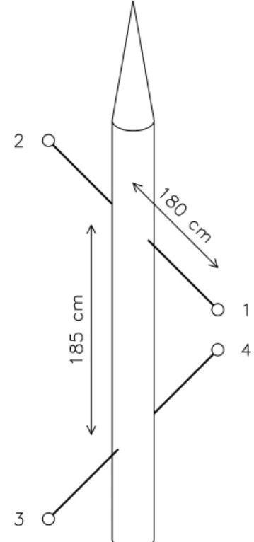
Fig. 1.Schematic diagram for the positioning of the probes on some instrumented rockets, with length scales relevant for the present analysis of data from the ROSE experiment (Rose et al., 1992).
In addition, we have a practical problem with rocket data: since no absolute potential reference (“ground”-potential) is available, potential variations have to be detected by taking the potential difference between two probes. In principle, potential variations could be measured with respect to the rocket body, but experience has shown that this gives rise to very “noisy” signals, presumably because the probes are in general outside the Mach cone, and the rocket body inside. The standard configuration (Bahnsen et al., 1978; Rose et al., 1992), as addressed also in this work, consists of booms car-rying the probes, as illustrated in Fig. 1, where the poten-tial differences can be obtained between probes on the same boom or alternatively between probes on different booms.
we “mimic” the signal as it would be obtained by a poten-tial difference measurement carried out by an instrumented rocket. For the ionospheric rocket only the latter option is available. Our analysis includes structure functions up to 8th order, being aware that the accuracy of the estimate decreases for increasing order.
Our analysis refers, as stated, to one particular plasma in-stability. The Farley-Buneman instability is driven by a cur-rent (i.e. the E0×B-electron flow through unmagnetized or
weakly magnetized ions), and is thus likely to have proper-ties in common with other current driven instabiliproper-ties. We therefore anticipate that our results are qualitatively relevant for other plasma instabilities.
2 Numerical simulations
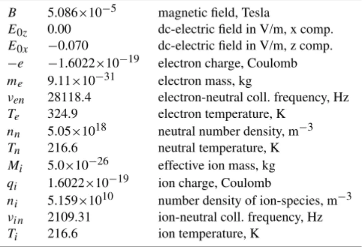
The numerical simulations were conducted in two spatial di-mensions in the plane perpendicular to the imposed mag-netic field, using a Particle-in-Cell (PIC) code (Birdsall and Langdon, 1991) for the ion component and a fluid model for the electrons (Oppenheim et al., 1995; Oppenheim and Otani, 1996; Dyrud et al., 2006). In the present analysis, the electron inertia is ignored. Details of the simulation code are presented by Oppenheim et al. (2003). We have per-formed also smaller box simulations with the same param-eters used in the simulations shown here, but with finite elec-tron inertia, and found no substantial difference in the re-sulting evolution or spectral characteristics of the present pa-rameters. The plasma parameters used in the present study are summarized in Table 1. For E0 we use the largest value that is relevant for the rocket experiment discussed in Sect. 4. For our conditions, the recombination coefficient isβR≈3×10⁻⁷cm−3s−1. Recombination effects are not in-cluded in the simulations, since they give only small correc-tions for the present strongly driven case (Fejer et al., 1984). We deal with low-β plasmas, and the magnetic field is as-sumed constant. We use a value for the electron temperature which is consistent with the present observations. Evidence can be found for anomalous electron temperature enhance-ments for increasing dc electric field in the ionospheric E-region (St.-Maurice et al., 1999; No¨el et al., 2005), where theeffectiveelectric field needs to be considered in case we have neutral winds. Unfortunately, we have no means for ob-taining information concerning neutral winds for the ROSE-experiment. ForE0≈40 mV/m, i.e. for the up-leg conditions of the rocket experiment discussed in Sect. 4, the increase inTe is expected to be minute, but for the somewhat larger down-leg fields,E0≈60–70 mV/m, nontrivial enhancements ofTe are anticipated, but not observed for the present con-ditions. The wave propagation velocities, for instance, as found by Iranpour et al. (1997), Krane et al. (2000) and Dyrud et al. (2006) are best explained by an electron temper-ature of approximately 400 K. Also other reports (Pfaff et al., 1992) noted the lack of electron temperature enhancements
Table 1.Input data for the numerical simulations.
B 5.086×10⁻⁵ magnetic field, Tesla
E0z 0.00 dc-electric field in V/m, x comp. E0x −0.070 dc-electric field in V/m, z comp. −e −1.6022×10⁻¹⁹ electron charge, Coulomb me 9.11×10⁻³¹ electron mass, kg
νen 28118.4 electron-neutral coll. frequency, Hz Te 324.9 electron temperature, K
nn 5.05×10¹⁸ neutral number density, m−3 Tn 216.6 neutral temperature, K Mi 5.0×10⁻²⁶ effective ion mass, kg qi 1.6022×10⁻¹⁹ ion charge, Coulomb
ni 5.159×10¹⁰ number density of ion-species, m−3 νin 2109.31 ion-neutral coll. frequency, Hz Ti 216.6 ion temperature, K
for conditions similar to ours. A previous study (Dyrud et al., 2006) attempted to explain the low electron temperatures by thermal conduction to the colder regions below the enhanced wave activity, but used too low numerical values for the elec-tron energy loss per collision, by taking this energy loss to be at most an order of magnitude larger than for inelastic collisions. By far, the dominant cooling rate is due to in-elastic collisions in the E-region. It may be that the analysis of Dyrud et al. (2006) applies for conditions in laboratory experiments, where the dominant collisional electron energy loss will usually be for elastic collisions with neutral inert gases. The collisional energy losses for elastic collisions are generally much smaller than for the inelastic collisions.
In the related rocket experiments over Greenland (Bahnsen et al., 1978; P´ecseli et al., 1989) the electron temperature was determined. The propagation speed for the fluctuations that was found there agreed well with the sound speed obtained by an average ion mass and the experimentally obtained elec-tron temperature (P´ecseli et al., 1989).
An illustrative result from the simulations is shown in Fig. 2 for three times in physical units,t=5, 10, and 22 ms. The axes are in physical units as well. We note the evolu-tion of small scale structures in the linear initial phase of the instability. Eventually, in the nonlinear phase, larger scale structures develop and a saturated turbulent stage of the instability is reached. Typically, the saturated potential fluctuations have a characteristic wavelength of∼2 m, and a peak value of∼0.3 V. A typical root-mean-square value of the potential fluctuations is ∼0.08 V, corresponding to ac-electric fields∼3×10⁻²E
0, for the given conditions. The
fluctuations in density are relatively modest, typically below 20%, even though we can observe larger spikes (Dyrud et al., 2006).
0
5
10 15 20 25
0
5
10
15
20
25
z (m)
0
5
10 15 20 25
0
5
10 15 20 25
x (m)
-0.4
-0.0
0.3
Phi (V
)
x (m)
x (m)
t = 5 ms
t = 10 ms
t = 22 ms
Fig. 2.Summary plots illustrating the electrostatic potential for three times as obtained from the numerical simulations. The magnetic field is perpendicular to the plane of the paper, and the E0×B-drift is in the vertical direction, with E0=70 mV/m in the positive x-direction.
100 200 300 400 −0.2
−0.1 0 0.1 0.2
Time [sample no.]
Amplitude
Fig. 3. Example of time series from the simulations. The ini-tial red part contains the non-stationary iniini-tial growth phase and is omitted from the analysis. We verified that our results are ro-bust with respect to small variations in the lengths of the omitted time-sequences.
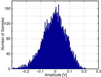
that the time-evolutions of the small scale structures are sta-tistically independent. Each of these samples contains ap-proximately 500 time steps. We omit the initial∼200 time samples when analyzing the data, since they contain an ini-tial non-stationary exponenini-tial growth phase. The ampli-tude probability density for the signals used in the analysis are given in Fig. 4. For this figure we used all data from the available points and all the time-series, except the initial omitted part. Figure 4 is thus an estimate of the one point amplitude probability density. The non-vanishing average in Fig. 4 is an indicator of the uncertainty due to the finite
num-−0.2 −0.1 0 0.1 0.2 0.3
0 40
80 120
160
Amplitude [V]
Number of Samples
Fig. 4.Amplitude probability density for the fluctuations. The lowest order moments are hφi= −7×10⁻³V, σφ ≡ h(φ − hφi)2i1/2=8×10−2V, S≡ h(φ− hφi)3i/σφ3= −3.29×10⁻¹, and K≡ h(φ− hφi)4i/σ4
φ=3.18.
100 101 102 100
101 102 103
Time difference [lag number]
Structure functions
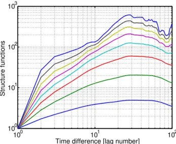
Fig. 5. Structure functions as functions of time separations (“time lags”), in units of numerical time samples. The electrostatic poten-tial is sampled in one fixed spapoten-tial position. The order parameter n=1. . .8 increases from bottom to top.
3 Data analysis
We study the structure functions associated with temporal and spatial variations of the signal. To study the time varia-tions, we consider a set of 25 time-series for the fluctuating potentialφobtained in a 5×5 grid with 3 m separation. This grid should not be confused with the simulation grid, which is much finer. To study the fixed-time spatial variations, we consider 25 samples with full spatial resolution, taken at dif-ferent times in the saturated stage.
3.1 One-point statistics for temporal variations
We obtain first the temporal structure functions h|φ (t1)−φ (t2)|ni for n=1,. . ., 8, with t1 and t2 being
two times in the same record. The averaging is performed over the individual time samples and then over the 25 sets of the data. Results are shown in Fig. 5 in a double logarithmic presentation. The structure functions are normalized to the first time sample. Note that forn≥7 we have a non-trivial uncertainty in the estimate of the corresponding structure function. We perform a power-law fittαn to these structure functions in the interval 3–10, showing in Fig. 6 the exponent αnfor different values ofn. By varying the length of the time interval used for obtaining the structure functions we find that the values ofαnup ton=6 are robust, while they become increasingly uncertain for larger n. For n>8, we do not consider the estimates forαn to be reliable. The power-law indexαn of the structure functions shown in Fig. 6 have a pronounced deviation from the linear relationship with n
0 2 4 6 8
0 0.5 1 1.5
n
α
n
Fig. 6.Exponents in the fittαnof the fixed-point temporal structure functions for different values ofn, see also Fig. 5. The power-law variation is fitted in the interval 3–10 time lags.
expected for Gaussian random signals. This deviation is conspicuous already forn=4. In Appendix B we give a more detailed discussion of the uncertainty of the estimators of the structure functions due to finite record lengths.
3.2 Two-point potential difference statistics, temporal vari-ations
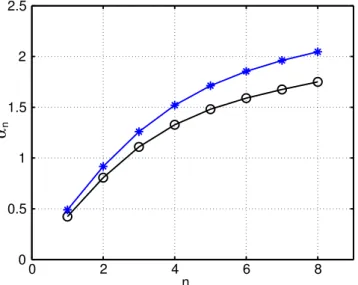
We note that the structure functions obtained by the forego-ing analysis can not be directly compared to rocket observa-tions as obtained by many instrumented rockets, for reasons outlined in the introduction. In order to make the analysis more directly relevant for comparisons with rocket data, we consider the potential difference between two positions sep-arated by 3 m, which is representative for many rocket ge-ometries, in particular also for those to be discussed later in this paper (Rose et al., 1992). This difference can be taken in basically two directions in the available two dimensional geometry. The corresponding values of the exponent are de-noted byα⊥andαk, respectively, where the subscripts⊥and krefer to the E0×B-direction. Figure 7 shows the variation
ofα⊥andαkwithn. We find these results to be significantly different from those summarized in Fig. 6. Thus, with rele-vant separations, the two-point difference signal has statisti-cal properties significantly different from those found when analyzing the one point signal.
0 2 4 6 8 0
0.5 1 1.5 2 2.5
n
α
n
Fig. 7. Variation withnof the two exponentsα⊥andαk, for the temporally varying potential difference structure functions, taken at two spatial positions separated by 3 m, in thex (asterixes) andz (circles) directions, respectively.
possible values of all the parameters entering the problem will make the analysis extremely lengthy. We argue in the following that the modifications are unlikely to be significant for the comparison with the available rocket data, to be dis-cussed later.
3.3 Structure functions for spatial separations at fixed times The analysis of Sect. 3.1 and 3.2 refers to temporal separa-tions when calculating the structure funcsepara-tions. Similar re-sults can be obtained by aspatialsampling of the potential at a fixed time, and then varying the separation.
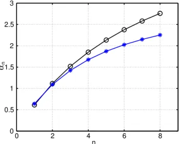
We now obtain the structure functions of the potential dif-ference between two spatial positions separated alongx and along z, respectively. Based on a set of 5 samples at dif-ferent times distributed over the available time-interval for the fluctuating potentialφin the entire available plane, we obtain the structure functions h|φ (x1, z)−φ (x2, z)|ni and h|φ (x, z1)−φ (x, z2)|ni for n=1, . . ., 8. The averaging is performed over the spatial samples and then over the 5 sets of data, taken at different times. Results are shown in Fig. 8 in a double logarithmic presentation. The exponents correspond-ing to the spatial structure functions are shown in Fig. 9 for differentn.
The relation between the spatio-temporal variation of the ionospheric signal and the time varying signal obtained from the rocket have already been discussed by P´ecseli et al. (1989). Basically, we find a Doppler shift due to the rocket motion and a frequency and amplitude modula-tion due to the rocket spin. If the rocket spin frequency is small as compared to relevant wave-frequencies (which
100 101 102
100 101 102 103 104 105
Distance [lag number]
Structure functions (x−direction)
100 101 102
100 101 102 103 104 105
Distance [lag number]
Structure functions (y−direction)
Fig. 8. Fixed-time structure functions as a function of spatial sep-arations, in units of numerical spatial samples. On top we have spatial separations in the z-direction (perpendicular toE0×B) and in the bottom for the x-direction (parallel toE0×B). The order parametern=1, . . ., 8 increases from bottom to top. Note that for n≥7 we have also here a non-trivial uncertainty in the estimate of the corresponding structure function.
0 2 4 6 8 0
0.5 1 1.5 2 2.5 3
n αn
Fig. 9. Variation withnof the two exponentsαxand αz, for the potential structure functions for spatial separations taken at a fixed time, see also Fig. 8. The power-law variation is fitted in the interval 3–15 spatial lags, except forn=8 where it is 3–12. The circles refer to the difference in the z-direction, asterixes to differences in the x-direction.
conditions, we find the following relation ∂2
∂t2
D
12φ (t )E≈(U·∇)2D1φ (r)2E, (7) with1φ (t )≡φ (t1)−φ (t2)and 1φ (r)≡φ (r1)−φ (r2), with t≡t1−t2 and r≡r1−r2. Alternatively, we can assume the observer to be fixed and the wave field to be propagat-ing with a large velocityU, and the Taylor hypothesis can again be applied. The plots in Fig. 2 indicate that all fre-quency components propagate uni-directionally, at least to a good approximation. The propagation velocity is ap-proximately the sound speed. In either case, the spatial and temporal correlation functions, and consequently also the corresponding structure functions, will be related as h12φ (r=0, t )i≈h12φ (r=Ut, t=0)i. If we assume that both h12φ (t )iandh12φ (r)ihave a power-law variation in a sig-nificant interval, we can argue by Eq. (7) that the characteris-tic exponentsαtandαzfor the two cases are directly related, αt≈αz, taking the z-coordinate to be alongU. By comparing Figs. 6 and 9 we find a reasonable agreement up ton=3 for the results argued on basis of the Taylor hypothesis. How-ever, the latter is not applicable on the structure functions for spatial separations perpendicular toU.
3.4 Discussion of the analysis of the simulation data We find that the first few values ofαnare close to be directly proportional ton, while forn>3 we find a pronounced de-viation from a linear variation. It thus seems that we have found a clear indication for intermittency effects in the tur-bulence. Forn=1, 2 the values ofα-exponents in Fig. 6 and 9
are close, indicating that the frozen turbulence approximation has a certain region of applicability, but also note that the dif-ferences increase rapidly withnas soon asn≥3, indicating that the higher order structure functions are very sensitive to deviations from the assumption of frozen turbulence. It is also interesting that forn=1 andn=2 we find no difference between the α-values in Fig. 9, which could be taken as a sign of spatial isotropy, i.e. lack of distinction between the x and z-directions for the smallest scales. This fact is consis-tent with an intermittency model based on secondary insta-bilities associated with gradients of larger scale structures, which are in turn again influenced by even larger scale struc-tures. When we approach the smallest scales being resolved, we have an approximate local isotropy of the spatial poten-tial variations. Similar observations have been made for elec-trostatic drift wave turbulence (Okabayashi and Arunasalam, 1977; P´ecseli, 1982), where similar arguments apply (Hal-latschek and Diamond, 2003).
4 Analysis of rocket data
We analyze data from the ROSE4 rocket (Rose et al., 1992). The ionospheric conditions and details of the instrumenta-tion relevant for the present dataset were discussed in a spe-cial issue of Journal of Atmospheric and Terrestrial Physics (54, 655–818, 1992). Here we present only a short sum-mary: dc-electric field values of typically 40 and 70 mV/m were measured by the rocket instruments on up-leg and down-leg passages of the E-region, respectively. The cor-responding E0×B/B2 velocities are approximately 800 and
1400 m/s. These values are of a sufficient magnitude to ex-cite the Farley-Buneman instability. The threshold value for the electric field is approximately 20 mV m−1.
The extremely low frequency (ELF) signals analyzed here were obtained by means of gold-plated spherical probes of 5 cm diameter, mounted on two pairs of booms, one near the top of the payload (labeled 1 and 2) and the other 185 cm lower (labeled 3 and 4), oriented at an angle of 90◦with re-spect to the first pair, as illustrated in Fig. 1 (Rinnert, 1992). The length of each boom was 180 cm. We analyzed the fol-lowing fluctuating signals
U6(t )=φ1(t )−φ2(t ), U5(t )=φ4(t )−φ3(t ), U4(t )=φ1(t )−φ4(t ), U3(t )=φ2(t )−φ3(t ), U2(t )=φ1(t )−φ3(t ), U1(t )=φ2(t )−φ4(t ),
Fig. 10. Structure functionsh1nφ (t )ifor varying ordern=1,. . ., 8 for the time interval 112.0–116.1 s, on the up-leg part of the flight.
becomes more complicated when the spectra contain wave-lengths comparable to or smaller than the probe separation. In general, the difference signal can be interpreted in terms of a filtering operation of the spatial potential variation.
The space-time varying electric field fluctuations of the electrojet were originally sampled with a 4 kHz sampling fre-quency. By averaging sampling points two-by-two, we here increased the sampling interval to 0.5 ms, giving a Nyquist frequency of 1000 Hz. The electric circuits give an effective frequency limitation being noticeable for frequencies larger than 600 Hz. The signals were digitized with 12 bit resolu-tion. Amplitudes of the potential differences were typically in the range 15–30 mV. The amplitudes of the relative den-sity fluctuations,en/n0, were in the range 1–3%. The
ampli-tude probability density of the detected potential difference fluctuations is non-Gaussian (Larsen et al., 2002), but it is important to emphasize that this conclusion refers to the fil-tered signal. The probability amplitude of the non-filfil-tered signal is, on the other hand, significantly affected by the rocket spin. We have analyzed all probe-combinations, but show here only results forU6, the differences between e.g. U6andU2being small, these two difference signals referring to probe-sets perpendicular to the rocket axis. For the small time separations relevant for the present analysis we do not find significant differences between signals such asU6 and U5either, but note that the correlation times for these signals
are somewhat different (Iranpour et al., 1997; Krane et al., 2000).
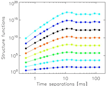
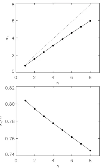
In Fig. 10 we show the structure functionsh1nφ (t )i for n=1,. . ., 8, as a function of temporal separations. These data are obtained from the up-leg part of the flight, where the fluctuation amplitude level is somewhat smaller than for the down-leg part. We note an overall similarity with the results
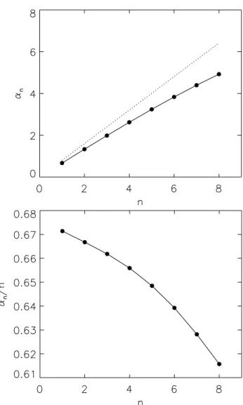
Fig. 11. Variation of the exponent with the order of the structure function, shown together with the corresponding variation of the compensated exponent for varying orders of the structure function, corresponding to Fig. 10. The time interval is 112.0–116.1 s, during the up-leg part of the flight. The dashed line on the figure forαn for varyingnis determined by the spectral index of the frequency power spectrum as discussed in the appendix.
obtained from numerical simulations (see Fig. 5). Also in the present case we can fit a power-lawtαnand show in Fig. 11 the variation ofαnwithn. The points lie on a curve which is close to a straight line, so we also show the compensated variationαn/n. In this representation, the deviations from the Gaussian results become more noticeable.
Fig. 12. Results for the synthetic data, corresponding to Fig. 11, showing the variation of the exponent with the order of the struc-ture function together with the corresponding variation of the com-pensated exponent for varying order of the structure function, cor-responding to Fig. 11. The green shaded areas represent a statistical scatter obtained by varying the seed of the random number genera-tors for the surrogate data.
randomizing the phase information by a standard random number generator. The power-spectrum of the resulting dataset is then the same as the one obtained for the origi-nal data, but the relative phases of the various Fourier com-ponents are unrelated to the previous ones. Coherent struc-tures that may be present in a signal will be characterized by distinct phase relations of their Fourier components. The randomization of the phases will consequently destroy such possible coherent structures. These surrogate data have ap-proximately Gaussian properties and the compensated
Fig. 13. Structure functions for the time interval 250.0–254.1 s on the down-leg part of the flight.
exponents αn/n should be approximately constant. The properties of the surrogate data depend also on the seed of the random number generators. In order to demonstrate the effects of this dependence, we generated many sets of syn-thetic data, and show the range of variability of the resulting values ofαnby a green-shaded area in Fig. 12. The thin red line gives the average curve. The results in Fig. 11 fall out-side the shaded region for largen, but only marginally so.
We extended the analysis to include also a sequence from the down-leg part of the flight in a time-interval 250.0– 254.1 s, where the overall fluctuation level is somewhat in-creased as compared to the up-leg part (Krane et al., 2000; Dyrud et al., 2006). In Fig. 13 we show the structure func-tions for varying order as funcfunc-tions of temporal separafunc-tions for this down-leg time interval. The analysis of the expo-nents have been carried out also for these data, as shown in Fig. 14. In particular, Fig. 15 displays the analysis of surro-gate data, as in Fig. 12. Also here, we show the statistical scatter by a green shading. The values ofαn found in the original dataset fall somewhat outside the shaded region, in particular for largen. The slight narrowing of the green areas in Figs. 15 and 12 are an artifact due to the finite number of realizations of the random number generator seeds. For the surrogate data, the statistical spread in the estimate onαn/n increases nonlinearly withn.
Fig. 14. Variation of the exponent with the order of the structure function, shown together with the corresponding variation of the compensated exponent for varying order of the structure function, corresponding to Fig. 13. The time interval is 250.0–254.1 s on the down-leg part of the flight.
4.1 Discussion of the analysis of the rocket data
Comparing the results from analyzing the data from the nu-merical simulations with the corresponding analysis from the rocket data we find somewhat similar results. The part of the analysis of the simulation data where a compari-son is appropriate (i.e. what concerns the potential differ-ences) the structure functions have a subrange characterized by a clear power law variation. The exponent varies sys-tematically with the order n of the structure function, but the compensated exponent is not a constant. The electro-jet turbulence is intermittent in the sense that it has mea-surable differences from the results expected for Gaussian random processes. This conclusion is supported by the analysis of the surrogate data, emphasizing the statistical
Fig. 15.Results for the synthetic data, showing the variation of the exponent with the order of the structure function together with the corresponding variation of the compensated exponent for varying order of the structure function. The results correspond to Fig. 14. The green shaded areas represent also here the statistical scatter ob-tained by varying the seed of the random number generators for the surrogate data.
significance of the results. It is however clear that the inter-mittency effects found in the numerical simulations are more evident than in the ionospheric data.
The approximate local isotropy of the smallest scales dis-cussed in Sect. 3.4 makes the rocket spin immaterial for the present analysis.
5 Conclusions
We have demonstrated the presence of a power-law subrange for the structure functions associated with the electrostatic potential in turbulent plasma fluctuations for conditions ap-propriate for the ionospheric E-region. We found clear in-dications for intermittent fluctuations in the sense that the power-law index for the structure functions of ordern devi-ates from a simple n-proportionality. These features are sum-marized in Figs. 6, 7 and 9. In order to explain the physical reason for the intermittency, we give particular attention to secondary instabilities developing on the gradients of larger scale structures (Sudan, 1983). We note that such secondary instabilities can be found also for other instabilities (Hal-latschek and Diamond, 2003). These secondary instabilities are, by nature, of a “bursty” appearance, requiring the pres-ence of local large scale gradients, associated with a long wavelength component. The presence of secondary instabil-ities could be anticipated already by inspections of Eq. (6), where the local gradients can be considered as being associ-ated with large scale waves. As evident from the analysis, our diagnostic is based on structure functions of the electrostatic potential. Other related works (Tam et al., 2005) are based on wavelet transforms. They studied the degree of intermittency on different scales and found electric field fluctuations to be more intermittent on smaller scales.
We can make a simple series expansion of the struc-ture function by takingφ (r, t ) ≈ φ (0, t )+ ∇φ (r, t )|r=0· r, and find, to the same approximation h12φ (r)i ≈ h(∇φ (r)|r=0 · r)2i, i.e. a variation with the square of the separation coordinate. Similarly, we can argue h12φ (t )i≈h(∂φ (t )/∂t|t=0)2it2, see also the discussion in
Appendix B. The origin of time (as well as of position) vari-ables is arbitrary because of the stationarity and homogene-ity of the turbulence. We observe neither anyt2nor an r2 dependence of the structure function, implying that the range of validity of the previous approximation is very limited, and most likely constrained by collisions. This collisional time-scale is not resolved by the simulation, nor by the sampling period of the rocket instruments. The relevant smallest length scales are not resolved by the simulations.
We found several interesting features of the ionospheric plasma turbulence. First of all, intermittency, as evidenced by a lack of proportionality between the exponentsαn and the ordernof the structure function, is much more evident for ionospheric turbulence as compared to turbulence in neutral incompressible flows (Anselmet et al., 1984). Forn≥4 there is a significant difference between the fixed-position tempo-ral intermittency (see Fig. 6) and the one associated with the fixed time spatial-difference variable (see Fig. 9). On the
other hand, we note some overall similarity between the vari-ation with the order parameternof the structure functions ob-tained for the time varying potential difference between two fixed positions (see Fig. 7), and the structure function taken at a fixed time with varying spatial separation (see Fig. 9), both cases referring to numerical simulations.
We find that the low frequency electrostatic turbulence in the ionospheric E-region is likely to be strongly intermittent for dc-electric field values that are common (i.e. in excess of 50 mV/m), but on the other hand we also find that stan-dard rocket probe set-ups, as illustrated in Fig. 1, are not well suited for recovering such features. Evidence for in-termittency can be found, but only by detailed investigations of the data, where the use of surrogate data can be an impor-tant tool for assessing the statistical significance of the results (Wernik, 1996).
The power-law exponentsαnwithn=1 found in the simu-lations are somewhat smaller than those for the rocket data, even when we consider the down-leg part which is most unstable, and the difference becomes more conspicuous for n≥2. The simulations show slightly stronger intermittency effects than the rocket data even when potential difference signals are considered. Part of the explanation deals with the sampling rate of the rocket data, which is too small to re-solve the smallest time-scales. Similarly, the grid-resolution and the finite time-step in the numerical simulations prohibit the finest details of the space-time variations of the physi-cal instability to be resolved completely. Considering these shortcomings, we might argue that the magnitudes of the ex-ponents αn for the simulations and the rocket observations forn=1 and 2 agree quite well.
The parameters chosen for the simulations are represen-tative for the most unstable conditions on the down-leg part of the rocket flight. If we average over the entire up-leg and down-leg parts, we find average electric fields smaller than the 70 mV/m used here. In spite of the strong fluctuation levels, we find that the detection method based on potential differences between two probes with a large separation gives signals that are close to exhibiting characteristics of Gaus-sian signals. We recover the strongly intermittent features only by making a one point analysis of the data. Rockets equipped as for the Rose campaign (Rose et al., 1992) are very useful for detecting the bulk features of plasma condi-tions and fluctuacondi-tions, but inadequate as soon as finer details, such as intermittency effects, of the E-region turbulence are studied. Some rockets, the TOPAZ II and TOPAZ III rock-ets for instance, has a somewhat different set-up (Vago et al., 1992) and it may be worthwhile to investigate the signals from these probes for studying intermittency effects.
slower one (P´ecseli et al., 1989). The transition is due to the change in electron dynamics, which is adiabatic for small aspect angles and isothermal for larger angles (P´ecseli et al., 1989). The zero aspect angle is likely to be a part of the earlier evolution of the amplitude. The full evolution of the structures may be three dimensional and such that once the amplitude has increased enough for the growth rate to slow down through the nonlinear effects (St.-Maurice and Hamza, 2001), then shears and rotations can introduce a fast evolv-ing aspect angle that destroys the structures while heatevolv-ing the electrons (J.-P. St.-Maurice, private communications, 2008). The largest amplitudes may be met when the phase speed has slowed down to be the threshold speed, i.e. isothermal ion-acoustic speeds at large aspect angles. Also the altitude dependence of the collision frequency can introduce an im-portant aspect angle effect on the properties of the non-linear wave structures as they approach saturation. We find it un-likely that these details can be recognized by an instrumen-tation as the one shown in Fig. 1, and foresee that numeri-cal simulations can have an important role in this discussion. The bulk of the rocket observations outlined here (although not in all detail, as discussed by Dyrud et al., 2006) can be accounted for by a two-dimensional numerical simulation as the one discussed in the present work.
We emphasize that the structure functions as obtained in the present study refer to relatively small spatial and short temporal scales. We might add a large amplitude, low fre-quency, long wavelength component which will make any signal significantly non-Gaussian, but such a wave will have negligible consequences on the present structure functions, by adding a slowly varying bias to our data.
Appendix A
The correlation function ρ is related to the power spec-trum S of the fluctuations by the Wiener-Khinchin theo-rem (Bendat, 1958). Considering the case with temporal variables we haveρ=ρ(τ )whereτ=t1−t2. The frequency
power spectrum is then obtained by the cosine transform of ρ(τ ). Assuming that we have a range {τa:τb}of τ-values whereρ≈1−Aταwe have
S(ω)=R0τaρ(τ )cos(ωτ )dτ+Rτb∞ρ(τ )cos(ωτ )dτ +Rτb
τa(1−Aτα)cos(ωτ )dτ
=R0τaρ(τ )cos(ωτ )dτ+Rτb∞ρ(τ )cos(ωτ )dτ +sin(ωτb)−sin(ωτa)
ω −
A
ωα+1
Rτbω
τaω γ
αcos(γ )dγ ,
(A1)
withγ≡ωτ.
For ω-intervals where the three integrals in Eq. (A1) are slowly varying with ω, we have a power spectrum S(ω)∼1/ωα+1 in that interval, relating the exponent in the power-spectrum to the exponent in the structure function.
If τa is small, we can approximate ρ≈1−12ρ′′τ2 and find, for instance, the first integral in Eq. (A1) to be (ω2+ρ′′(1−τa2ω2/2))sin(τaω)/ω3−ρ′′τacos(τaω)/ω2, which varies slowly withωwhenω>1/τa. For the particular, idealized, case whereρ has a “cusp” at the origin, we have ρ≈1−Aταfor smallτ∈{0:τb}, and can simplify Eq. (A1) as
S(ω)=Rτb∞ρ(τ )cos(ωτ )dτ+R0τb(1−Aτα)cos(ωτ )dτ =Rτb∞ρ(τ )cos(ωτ )dτ+
sin(ωτb) ω −ωαA+1
Rτbω
0 γαcos(γ )dγ ,
(A2)
where the second term is small whenα>1. The integrals in the last terms of Eqs. (A1) and (A2) have analytical, but lengthy, expressions. For instance, the integral in the last term in Eq. (A2) is found to be slowly varying withω<1/τb. The applicability of the approximations Eq. (A1) as well as Eq. (A2) are restricted by the requirement thatS(ω)≥0. By the dashed lines in Figs. 11 and 14 we give the slope of line nαdetermined by fittingω−α−1to the power-law spectrum for largeω.
For spatial separations, we have similar expressions in terms of wavenumbers (Hinze, 1975). If we, as an illustra-tion, consider again the universal range of the second order structure function in fully developed incompressible turbu-lence, we have an∼(ǫr)2/3variation in terms of the sepa-rationr and the specific energy dissipation rateǫ, while the wave-number power spectrum varies as∼ǫ2/3k−5/3,
consis-tent also with the foregoing estimates.
A spectral representation can be convenient from an ex-perimental point of view and several studies of plasma tur-bulence analyzed turbulent spectra. Results from laboratory experiments that were particularly relevant for the E-region fluctuations (Mikkelsen and P´ecseli, 1980; P´ecseli et al., 1983) have been compared to spectra obtained from rocket experiments (Krane et al., 2000).
Appendix B
The present appendix deals with the consequences of finite time sequences for the estimates of the structure functions. The analysis is limited by considering only a time-varying signal. We consider this as an insignificant restriction.
Taking one record, we can obtain an estimate for the n-th order structure functionEn=T1 R0T 1nφ (t1, t1+τ )dt1,
where1φ (ta, tb)≡|φ (ta)−φ (tb)|, noting the implied simpli-fying assumption that the integration intervalT is indepen-dent ofτ. The estimateEn=En(T, τ )is statistically vary-ing over the ensemble of realizations (Bendat, 1958; P´ecseli, 2000). It has an average value
hEni=1 T
Z T
0 h
1nφ (t1, t1+τ )idt1, (B1)
We now assume that the process is time stationary. We then have h1nφ (t1, t1+τ )i=h1nφ (0, τ )i≡9n(τ ) indepen-dent oft1, givinghEni=9n(τ ), since the integral in Eq. (B1) becomes trivial. This result forhEniwill be used in the fol-lowing.
The estimate En has a statistical variance σn≡q(En−hEni)2,which we can determine by
σn2=T1 R0T 1nφ (t1, t1+τ )dt1−9n(τ )
2
=hQT(τ )i−9n2(τ )
(B2)
where hQT(τ )i =
1 T2 Z T 0 Z T 0
1nφ (t1, t1+τ )1nφ (t2, t2+τ )dt1dt2≡
1 T2 Z T 0 Z T 0 ℵn
(τ, t1, t2)dt1dt2
. (B3)
We again make use of the time stationarity of the pro-cess, which impliesℵn(τ, t1, t2)=ℵn(τ,0, t2−t1)≡ℵn(τ, ν), with ν≡t2−t1. We also have ℵn(τ, ν)=ℵn(−τ, ν) and ℵn(τ, ν)=ℵn(τ,−ν). We can now write
hQT(τ )i = 1
T2
RT
0
RT
0 ℵn(τ,0, t2−t1)dt1dt2 =T12
RT
0
Rt2
t2−T ℵn(τ, ν)dνdt2.
(B4)
Reversing the order of integration (Bendat, 1958) we readily find
hQT(τ )i = 1
T2
R0 −T
RT+ν
0 ℵn(τ, ν)dνdt2 +T12
RT
0
RT
t2 ℵn(τ, ν)dνdt2.
(B5)
We now note that R0
−T
RT+ν
0 ℵn(τ, ν)dνdt2=
RT
0
RT−ν
0 ℵn(τ, ν)dνdt2,
and consequently havehQT(τ )i= 2
T2
RT
0 (T−ν)ℵn(τ, ν)dν,
which gives σn2= 2
T2
Z T
0
(T−ν)
ℵn(τ, ν)−9n2(τ )
dν. (B6)
We usedT22
RT
0 (T−ν) dν=1.
The expression in Eq. (B6) assumes knowledge of ℵn(τ, ν), which is not necessarily available. We can consider some special limiting cases. First we as-sume that τ is small, so we can make the ap-proximation1φ (ta, tb)≡|φ (ta)−φ (tb)|≈|φa| |′ ta−tb|, where φa≡′ dφ/dt|t=ta. In the limit of small τ we have 9n(τ ) ≈ h|φ′|niτn, where we here can omit the subscript onφ′ be-cause of the assumed time-stationarity of the process. Simi-larly, we haveℵn(τ, ν)≈h|φ′1|n|φ2′|niτ2nfor smallτ. Conse-quently, we have for this limiting case
σn2=2τ 2n
T2
Z T
0
(T−ν)
h|φ1′|n|φ2′|ni−h|φ′|ni2
dν, (B7)
0
5
10
15
20
25
Τ
c0
0.2
0.4
0.6
0.8
1
Σ
nΤ
nΦ
'
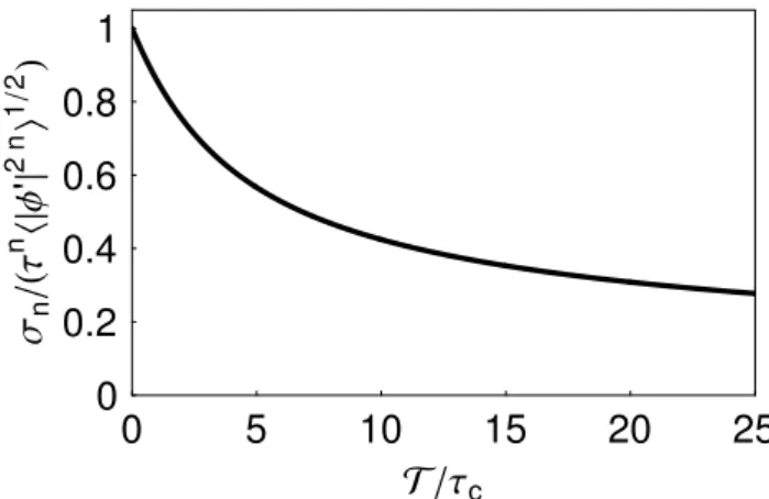
2 n 1 2Fig. B1.Variation of the normalized varianceσn/
τnh|φ′|2ni1/2
withT/τc. We used an exponential model for the correlation func-tion for|φ′|.
whereh|φ1′φ2′|niimplicitly depends on ν≡t2−t1. For large ν where φ1 and φ2 can be assumed to be statistically in-dependent, we have h|φ′1|n|φ2′|ni≈h|φ1′|nih|φ2′|ni=h|φ′|ni2, so the integrand vanishes in this limit. At ν≈0 we have h|φ1′|n|φ2′|ni≈h|φ′|2ni≥h|φ′|ni2by the Schwartz-Cauchy in-equality.
The result Eq. (B7) demonstrates that the root-mean-square errorσnincreases with time separation asτnfor con-stantT. This observation can be used for fixedτand varying n, or vice versa.
In order to illustrate the variation with T, we postulate a simplified model of the correlation function for |φ′|n in the formρn(ν)≈h|φ′|2niexp(−|ν|/τc)+h|φ′|ni2,withτc be-ing a correlation time, and use this model in Eq. (B7). The proposed correlation function will be accurate for the case where the potential derivative |φ′| is a random Gaussian Markov process with non-zero mean (Bendat, 1958; P´ecseli, 2000). In Fig. B1 we show the variation of the normalized variance σn
The present analysis assumes smallτ. For arbitraryτ we have to model the entire variation ofℵn(τ, ν). This will not be discussed here. A discussion of the uncertainty of the estimate of structure functions for the spatial variations of the potential at a given fixed time can be carried out as shown before and need not be discussed here.
The error estimates discussed in this appendix assumes that we have one time record available. In the numerical simulations discussed in Sect. 2 we had 25 such records of equal lengths. The estimate En can be generalized as En=N1 PNm=1 1
T
RT
0 1
nφ
m(t1, t1+τ )dt1, with m being the
label of the record. In our case we haveN=25. If we can assume the N records to be statistically independent (in prac-tice by assuming that they are obtained at positions separated by more than a correlation distance), it is relatively straight-forward to generalize the foregoing analysis. We find that the errorσnscales as∼1/
√ N.
The present appendix assumes continuous functions, where we in our foregoing analysis had sampled space-time varying functions. It is however evident even from the present appendix that the number of samples alone can not determine the accuracy of an estimate. If we have a very dense sampling within a time sequence shorter than the cor-relation time, our estimate will be inaccurate under all cir-cumstances. It is important to distinguish the number of samples of1φ (ta, tb)≡|φ (ta)−φ (tb)|obtained from differ-ent and statistically independdiffer-ent realizations, and the number of time samples in one record.
Acknowledgements. This work was in part supported by the Norwegian National Science Foundation. The work by L. Dyrud and M. Oppenheim was partially supported by US National Science Foundation Grant ATM-0442075. The Rocket and Scatter Experiment (ROSE) was performed in the framework of the German national sounding rocket program with international participation. It was primarily funded by the Bundesministerium f¨ur Forschung und Technologie (BMFT) and was managed by the Deutsche Gesellschaft f¨ur Luft- und Raumfahrt (DLR). One of the authors (HLP) thanks Jean-Pierre St.-Maurice for valuable communications.
Edited by: A. C. L. Chian
Reviewed by: two anonymous referees
References
Anselmet, F., Gagne, Y., Hopfinger, E. J., and Antonia, R. A.: High-order velocity structure functions in turbulent shear flows, J. Fluid Mech., 140, 63–89, 1984.
Bahnsen, A., Ungstrup, E., F¨althammer, C.-G., Fahleson, U., Ole-sen, J. K., Primdahl, F., Spangslev, F., and PederOle-sen, A.: Elec-trostatic waves observed in an unstable polar cap ionosphere, J. Geophys. Res., 83, 5191–5197, 1978.
Bendat, J. S.: Principles and Applications of Random Noise Theory, John-Wiley & Sons, New York, 431 pp., 1958.
Birdsall, C. and Langdon, A.: Plasma Physics via Computer Simu-lation, Adam Hilger, Bristol, 479 pp., 1991.
Boedo, J. A., Rudakov, D. L., Moyer, R. A., McKee, G. R., Colchin, R. J., Schaffer, M. J., Stangeby, P. G.and West, W. P., Allen, S. L., Evans, T. E., Fonck, R. J., Hollmann, E. M., Krasheninnikov, S., Leonard, A. W., Nevins, W., Mahdavi, M. A., Porter, G. D., Ty-nan, G. R., Whyte, D. G., and Xu, X.: Transport by intermittency in the boundary of the DIII-D tokamak, Phys. Plasmas, 10, 1670– 1677, 2003.
Bruno, R. and Carbone, V.: The solar wind as a turbulence lab-oratory, Living Reviews in Solar Physics, 2, available at: http: //www.livingreviews.org/lrsp-2005-4, 2005.
Buneman, O.: Excitation of field aligned sound waves by electron streams, Phys. Rev. Lett., 10, 285–287, 1963.
Chandrasekhar, S.: The theory of turbulence, Journal Madras Uni-versity, B 27, 251–275, 1957.
Chang, T. and Wu, C.-C.: Rank-ordered multifractal spec-trum for intermittent fluctuations, Phys. Rev. E, 77, 045 401, doi:10.1103/PhysRevE.77.045401, 2008.
Chen, F. F.: Spectrum of low-βplasma turbulence, Phys. Rev. Lett., 15, 381–383, 1965.
Dyrud, L., Krane, B., Oppenheim, M., P´ecseli, H. L., Schlegel, K., Trulsen, J., and Wernik, A. W.: Low-frequency electrostatic waves in the ionospheric E-region: a comparison of rocket ob-servations and numerical simulations, Ann. Geophys., 24, 2959– 2979, 2006
Dyrud, L. P., Oppenheim, M. M., Close, S., and Hunt, S.: Interpre-tation of non-specular radar meteor trails, Geophys. Res. Lett., 29, 2012, doi:10.1029/2002GL015953, 2002.
Farley, D. T.: Two-stream plasma instability as a source of irregu-larities in the ionosphere, Phys. Rev. Lett., 10, 279–282, 1963. Fejer, B. G. and Kelley, M. C.: Ionospheric irregularities,Rev.
Geo-phys.,18, 401–454, 1980.
Fejer, B. G., Providakes, J., and Farley, D. T.: Theory of plasma waves in the auroralEregion,J. Geophys. Res.,89, 7487–7494, 1984.
Fredriksen, ˚A., Riccardi, C., Cartegni, L., Draghi, D., Trasarti-Battistoni, R., and Roman, H. E.: Statistical analysis of tur-bulent flux and intermittency in the nonfusion magnetoplasma Blaamann,Phys. Plasmas,10, 4335–4340, 2003a.
Fredriksen, ˚A., Riccardi, C., Cartegni, L., and P´ecseli, H.: Coherent structures, transport and intermittency in a magnetized plasma, Plasma Phys. Contr. Fusion,45, 721–733, 2003b.
Hallatschek, K. and Diamond, P. H.: Modulational instability of drift waves,New J. Phys.,5, 29.1–29.9, 2003.
Hinze, J. O.: Turbulence, McGraw Hill, New York, 2 edn., 1975. Huld, T., Nielsen, A. H., P´ecseli, H. L., and Juul Rasmussen, J.:
Coherent structures in two-dimensional turbulence,Phys. Fluids B,3, 1609–1625, 1991.
Iranpour, K., P´ecseli, H. L., Trulsen, J., Bahnsen, A., Primdahl, F., and Rinnert, K.: Propagation and dispersion of electrostatic waves in the ionospheric E region,Ann. Geophys.,15, 878, 1997. Kervalishvili, G. N., Kleiber, R., Schneider, R., Scott, B. D., Grulke, O., and Windisch, T.: Intermittent turbulence in the lin-ear VINETA device,Contrib. Plasma Phys.,48, 32–36, 2008. Krane, B., P´ecseli, H. L., Trulsen, J., and Primdahl, F.:
Spec-tral properties of low-frequency electrostatic waves in the iono-spheric E region,J. Geophys. Res.,105, 10 585–10 601, 2000. Larsen, Y., Hanssen, A., Krane, B., P´ecseli, H. L., and Trulsen, J.:
doi:10.1029/2001JA900125, 2002.
Mikkelsen, T. and P´ecseli, H. L.: Strong turbulence in partially ion-ized plasmas, Phys. Lett. A, 77, 159–162, 1980.
No¨el, J.-M., St.-Maurice, J.-P., and Blelly, P.-L.: The effect of E-region wave heating on electrodynamical structures, Ann. Geo-phys., 23, 2081–2094, 2005,
http://www.ann-geophys.net/23/2081/2005/.
Okabayashi, M. and Arunasalam, V.: Study of drift-wave turbu-lence by microwave scattering in a toroidal plasma, Nucl. Fusion, 17, 497–513, 1977.
Oppenheim, M. and Otani, N.: Spectral characteristics of the Farley-Buneman instability: Simulations versus observations, J. Geophys. Res., 101, 24 573–24 582, 1996.
Oppenheim, M., Otani, N., and Ronchi, C.: Hybrid simulations of the saturated Farley-Buneman instability in the ionosphere, Geo-phys. Res. Lett., 22, 353–356, 1995.
Oppenheim, M. M., Dyrud, L. P., and vom Endt, A. F.: Plasma instabilities in meteor trails: 2-D simulation studies, J. Geophys. Res., 108, 1064, doi:10.1029/2002JA009549, 2003.
P´ecseli, H. L.: Drift-wave turbulence in low-β plasmas, Phys. Scripta, T2/1, 147–157, 1982.
P´ecseli, H. L.: Fluctuations in Physical Systems, Cambridge Uni-versity Press, Cambridge, UK, 190 pp., 2000.
P´ecseli, H. L. and Trulsen, J.: On the interpretation of experimen-tal methods for investigating nonlinear wave phenomena, Plasma Phys. Contr. Fusion, 35, 1701–1715, 1993.
P´ecseli, H. L., Mikkelsen, T., and Larsen, S. E.: Drift wave turbu-lence in a low-βplasma, Plasma Phys., 11, 1173–1197, 1983. P´ecseli, H. L., Primdahl, F., and Bahnsen, A.: Low-frequency
elec-trostatic turbulence in the polar cap E region, J. Geophys. Res., 94, 5337–5349, 1989.
Pfaff, R. F., Sahr, J., Providakes, J. F., Swartz, W. E., Farley, D. T., Kintner, P. M., H¨aggstr¨om, I., Hedberg, A., Opgenoorth, H., Holmgren, G., McNamara, A., Wallis, D., Whalen, B., Yau, A., Watanabe, S., Creutzenberg, F., Williams, P., Nielsen, E., Schlegel, K., and Robinson, T. R.: The E region rocket/radar instability study (ERRIS): scientific objectives and campaign overview, J. Atmos. Terr. Phys., 54, 779–808, 1992.
Rinnert, K.: Plasma waves observed in the Auroral E region ROSE campaign, J. Atmos. Terr. Phys., 54, 683–692, 1992.
Rogister, A. and D’Angelo, N.: Type II irregularities in the equato-rial electrojet, J. Geophys. Res., 75, 3879–3887, 1970.
Rollefson, J. P.: On Kolmogorov’s theory of turbulence and inter-mittency, Can. J. Phys., 56, 1426–1441, 1978.
Rose, G., Schlegel, K., Rinnert, K., Kohl, H., Nielsen, E., Dehmel, G., Friker, A., Lubken, F. J., L¨uhr, H., Neske, E., and Steinweg, A.: The ROSE project – scientific objectives and discussion of 1st results, J. Atmos. Terr. Phys., 54, 657–667, 1992.
Schreiber, T. and Schmitz, A.: Surrogate time series, Physica D, 142, 346–382, 2000.
Shkarofsky, I. P.: Turbulence in Fluids and Plasmas, “Analytic forms for decaying turbulence functions”, Polytechnic Press, Brooklyn, NY, USA, chap. 21, 1969.
St.-Maurice, J.-P. and Hamza, A. M.: A new nonlinear approach to the theory of E region irregularities, J. Geophys. Res., 106, 1751–1759, 2001.
St.-Maurice, J.-P., Cussenot, C., and Kofman, W.: On the useful-ness of E region electron temperatures and lower F region ion temperatures for the extraction of thermospheric parameters: a case study, Ann. Geophys., 17, 1182–1198, 1999
Sudan, R. N.: Unified theory of type-I and type-II irregularities in the Equatorial electrojet, J. Geophys. Res., 88, 4853–4860, 1983. Tam, S. W. Y., Chang, T., Kintner, P. M., and Klatt, E.: Intermit-tency analyses on the SIERRA measurements of the electric field fluctuations in the auroral zone, Geophys. Res. Lett., 32, L05109, doi:10.1029/2004GL021445, 2005.
Tu, C. Y. and Marsch, E.: MHD structures, waves and turbulence in the Solar-wind-observations and theories, Space Sci. Rev., 73, 1–210, 1995.
Vago, J. L., Kintner, P. M., Chesney, S. W., Arnoldy, R. L., Lynch, K. A., Moore, T. E., and Pollock, C. J.: Transverse ion accel-eration by localized lower hybrid waves in the topside auroral ionosphere, J. Geophys. Res., 97, 16 935–16 957, 1992. Wernik, A. W.: Methods of data analysis for resolving nonlinear
phenomena, in: Modern Ionospheric Physics, edited by Kohl, H., R¨uster, R., and Schlegel, K., European Geophysical Society, Katlenburg-Lindau, Germany, 321–345, 1996.