Nonlinear Container Ship Model for the Study of Parametric Roll Resonance

Nonlinear Container Ship Model

for the Study of Parametric Roll Resonance

Christian Holden

Roberto Galeazzi

Claudio Rodríguez

Tristan Perez

Thor I. Fossen

Mogens Blanke

Marcelo de Almeida Santos Neves

1_{Department of Engineering Cybernetics, Norwegian University of Science and Technology, Norway. E-mail:} {c.holden, fossen}@ieee.org

2_{Department of Electical Engineering, Technical University of Denmark. E-mail: {rg, mb}@elektro.dtu.dk}

3_{Department of Naval Architecture and Ocean Engineering, LabOceano/COPPE, Federal University of Rio de}

Janeiro, Brazil. E-mail: {claudiorc, masn}@peno.coppe.ufrj.br

4_{Centre for Complex Dynamic Systems and Control, University of Newcastle, Australia. E-mail: [email protected]} 5_{Centre for Ships and Ocean Structures, Norwegian University of Science and Technology, Norway.}

Abstract

Parametric roll is a critical phenomenon for ships, whose onset may cause roll oscillations up to ±40◦_,

leading to very dangerous situations and possibly capsizing. Container ships have been shown to be particularly prone to parametric roll resonance when they are sailing in moderate to heavy head seas.

AMatlab/Simulinkr_{parametric roll benchmark model for a large container ship has been implemented}

and validated against a wide set of experimental data. The model is a part of aMatlab/SimulinkToolbox (MSS, 2007). The benchmark implements a 3rd_{-order nonlinear model where the dynamics of roll is}

strongly coupled with the heave and pitch dynamics. The implemented model has shown good accuracy in predicting the container ship motions, both in the vertical plane and in the transversal one. Parametric roll has been reproduced for all the data sets in which it happened, and the model provides realistic results which are in good agreement with the model tank experiments.

Keywords: parametric roll resonance; nonlinear systems; model validation; parameter identification; ships

1 Introduction

Parametric roll is an autoparametric resonance phe-nomenon whose onset causes a sudden rise in roll os-cillations. The resulting heavy roll motion, which can reach 30-40 degrees of roll angle, may bring the vessel into conditions dangerous for the ship, the cargo, and the crew. The origin of this unstable motion is the time-varying geometry of the submerged hull, which produces periodic variations of the transverse stability properties of the ship.

Parametric roll is known to occur when a ship sails

in moderate to heavy longitudinal or oblique seas; the wave passage along the hull and the wave excited ver-tical motions result in variations of the intercepted wa-terplane area, and in turn, in relevant changes in the restoring characteristics. The onset and build-up of parametric roll is due to the occurrence of concomi-tant conditions: the wave length is close to the ship length (λw ≈ LPP), the ship approaches waves with

encounter frequency almost twice the roll natural fre-quency(ωe≈2ω0), and the wave height is greater than

The risk of parametric roll has been known to the maritime community since the early fifties, but only for small vessels with marginal stability – e.g. fishing boats – sailing in following seas. However, the phe-nomenon has recently attracted significant interest by the scientific community after accidents occurred with container ships sailing in head seas, incidents that in-volved significant damage to cargo as well as structural damages for millions of dollars (France et al., 2001; Carmel, 2006).

Several different types of vessel have reported to ex-perience parametric roll in head seas, e.g. destroyers (Francescutto, 2001), ro-ro paxes (Francescutto and Bulian, 2002) andPCTC(Palmquist and Nygren, 2004). Container carriers, however, are the most prone to parametric roll because of the current particular hull shape, i.e. large bow flare and stern overhang, and hence abrupt variation in the intercepted water-plane area when a wave crest or trough is amidships.

This has called for deep investigations into the na-ture of parametric roll in head/near head seas, and for the development of mathematical models able to capture and reproduce the physical aspects driving the resonant motion. In the last six years mathematical models of different complexity have been proposed by the scientific community, most of them relying on the Mathieu Equation to describe the dynamics of the ship subject to parametric resonance.

One-DOF models considering the uncoupled roll mo-tion have been widely used to analyze the critical pa-rameters of the phenomenon and derive stability condi-tions. Examples can be found in the papers by France et al. (2001) and Shin et al. (2004) where the authors employed the 1-DOF roll equation to show that, in regular waves, the Mathieu Equation can explain the onset of heavy roll motion in head seas.

Bulian (2006) proposed a 1.5-DOF model where the dynamic interaction between the vertical motions and the roll oscillation was relaxed by the assumption of quasi-static heave and pitch. Moreover, that assump-tion allowed an analytical descripassump-tion of the GZ curve that was approximated as a surface varying with roll angle and wave crest position. This model is consid-ered valid for moderate ship speed in head seas, and has lead to reasonable results in predicting parametric roll.

A 3-DOF nonlinear fully coupled model was first de-veloped by Neves (2002). A first attempt was done by using Taylor series expansion up to 2nd_{-order to}

describe the coupled restoring forces and moments in heave, pitch and roll. This model, although it provided a quite thorough description of the nonlinear interac-tions among the different modes, tended to overesti-mate the roll oscillation above the stability threshold.

Neves and Rodríguez (2005) proposed a 3rd_-order

an-alytical model where the couplings among the three modes are expressed as a 3rd_{-order Taylor series}

ex-pansion. In this new model the nonlinear coefficients are mathematically derived as a functions of the char-acteristics of the hull shape. This 3-DOF model has been applied for the prediction of parametric roll to a transom stern fishing vessel (Neves and Rodríguez, 2006a,b) providing outcomes which better match the experimental results than the2nd_{-order model.}

It is noted that the above-mentioned literature have attempted to model parametric roll from an analytical points of view. Jensen (2007) takes a statistical ap-proach instead, motivated by the difficulties inherent in describing the interaction between a 3-dimensional wave pattern and the motion of a ship hull. He shows how the statistical distribution of nonlinear ship re-sponses can be estimated very accurately using a first-order reliability method. A commercial implementa-tion in a system to predict parametric roll (SeaSenser₎

was reported in Nielsen et al. (2006).

The direction of this paper is the analytical one, aim-ing at providaim-ing simulation tools that could e.g. be used in studies of active stabilization and control. The model proposed by Neves and Rodríguez (2005) is ap-plied to describe the dynamics of a container vessel subject to parametric roll resonance conditions. The model parameters are identified based upon the ship line drawings and the loading conditions. A Matlab/

Simulink implementation of the above model is then presented. The reliability of the implemented model in simulating parametric resonance behavior is validated against experimental data. The validation has shown good agreement with the experimental results for roll both in the experiments where parametric roll reso-nance occurred, and in the experiments where it did not occur.

The main goal of this work is to provide a bench-mark for simulating parametric roll of a container ship over a large range of ship speeds and sea states. This benchmark has been designed to be a fully integrated part of Matlab/Simulink Toolbox for marine systems (MSS, 2007). The availability of such a powerful tool opens up a great wealth of opportunities, notably the design and testing of novel model-based roll motion stabilizers.

2 Mathematical Model for

Parametric Roll

physical laws governing that phenomenon and/or ex-perimental results.

Tondl et al. (2000) define an autoparametric system as follows:

Definition 1 _{Autoparametric systems are vibrating}

sys-tems that consist of at least two constituting subsys-tems. One is the primary system that will usually be in a vibrating state. This primary system can be ex-ternally forced, self-excited, parametrically excited, or a combination of these. The second constituting sub-system is called the secondary system. The secondary system is coupled to the primary system in a nonlinear way, but such that the secondary system can be at rest while the primary system is vibrating.

An autoparametric system is, hence, characterized by these main aspects:

1. two nonlinearly coupled subsystems;

2. a normal mode where the primary system is in a vibrating state and the secondary system is at rest;

3. the presence of instability regions where the nor-mal mode becomes unstable;

4. in the region of instability of the normal mode the overall system is in autoparametric resonance: the secondary system is parametrically excited by the vibrations of the primary system and it will not be at rest anymore.

Considering Definition 1, 1 DOF models have too lit-tle complexity to describe an autoparametric system, since the roll motion for a ship sailing in longitudinal seas represents only the secondary system. They are useful to obtain insight in the parametric roll resonance phenomenon, but they will have difficulty predicting the real amplitude of the oscillations about the trans-verse plane.

The model proposed by Neves and Rodríguez (2005) is complex enough to capture the dynamics of a con-tainer vessel behaving as an autoparametric system; it includes both the primary system (heave and pitch dynamics) which is externally excited by the wave mo-tion, and the secondary system (roll dynamics) which is parametrically excited by the primary.

2.1 Equations of Motion

The 3-DOF nonlinear mathematical model of the con-tainer vessel is presented in the following way (using the notation of Neves and Rodríguez (2005)):

Let

s_{(t) =}

z(t) φ(t) θ(t) T

(1)

be the generalized coordinate vector, where z is the heave displacement, φ is the roll angle, and θ is the pitch angle, as shown in Figure 1.

Figure 1: Definition of motions

Then the nonlinear equations of motion can be ex-pressed in matrix form as

(M₊A_)¨s₊B_{( ˙φ)˙}s₊c_res(s_{, ζ) =}c_ext(ζ,ζ,˙ _ζ¨_{) (2)}

where

• M_∈R3×3_{is the diagonal rigid-body generalized}

mass matrix;

• A_∈R3×3_{is the generalized added mass matrix;}

• B_∈R3×3_{is the hydrodynamic damping}

(nonlin-ear in roll);

• c_{res ∈ R}3 _{is the nonlinear vector of restoring}

forces and moments expressed as functions of the relative motion between ship hull and wave ele-vation ζ(t);

• c_{ext ∈ R}3 _{is the vector of the external wave}

ex-citation forces and moments which depends on wave heading, encounter frequency, wave ampli-tude and time.

2.1.1 Generalized Mass, Added Mass and Damping

The generalized mass matrix can be written as

M₌





m 0 0

0 Ix 0

0 0 Iy



 (3)

The hydrodynamic added mass and damping matri-ces are expressed as

A₌





−Zz¨ 0 −Z_θ¨

0 −K_φ¨ 0

−Mz¨ 0 −Mθ¨ 

 (4)

B_{( ˙φ) =}





−Zz˙ 0 −Zθ˙

0 −K_φ˙( ˙φ) 0

−Mz˙ 0 −M_θ˙ 

 (5)

where all entries except K_φ˙( ˙φ) can be evaluated by

means of potential theory (Salvesen et al., 1970). The hydrodynamic damping in roll may be expressed as

K_φ˙( ˙φ) ˙φ=K_φ˙φ˙+K_φ˙_|φ˙_|φ˙|φ˙| (6)

where the linear term represents the potential and lin-ear skin friction, whereas the nonlinlin-ear term takes into account viscous effects. The coefficientsK_φ˙ andK_φ˙_|φ˙_|

can be calculated by the formulae given in Himeno (1981). The roll damping characteristics may also be derived from data of roll decaying tests at appropriate forward speeds of the vessel.

2.1.2 Waves

In regular seas, the incident wave elevation according to the Airy linear theory, see Newman (1977), is defined as

ζ(x, y, t;χ) =Awcos(kxcosχ−kysinχ−ωet) (7) where Aw is the wave amplitude,k is the wave num-ber, χ is the wave heading, and ωe is the encounter wave frequency. For head seas (χ = 180◦_{), the wave}

elevation reads as

ζ(x, t) =Awcos(kx+ωet). (8)

2.1.3 Nonlinear Restoring Forces and Moments

The nonlinear restoring actions are given by the com-bination of the effects of the vessel motion in calm wa-ter and the effect of the wave elevation along the hull. Therefore, the vector of restoring forces and moments can be written, up to3rd_{-order terms, as}

c_pos≈c_pos,s+cpos,ζ

+c_pos,s2+cpos,sζ+c_pos,ζ2

+c_pos,s3+cpos,s2ζ+cpos,sζ2+cpos,ζ3

(9)

wherec_pos,si_ζj =∂ i+j_c

pos

∂si∂ζj s

i_ζj_.

The1st_,2nd _and3rd_{-order components in (9), which}

are independent of the displacement vectors_{, must be}

included in the external forces and moments acting on the vessel. These terms describe the linear and nonlin-ear Froude-Krylov forces/moments.

The2nd _and3rd_{-order nonlinear effects due to}

hull-wave interactions must, instead, be included in the restoring vectorc_{res because of their affinity, from the}

mathematical point of view, with the hydrostatic ac-tions. Then the restoring force and moments due to body motion are given by

c_res(s_{, ζ) =}c_pos(s_{, ζ)−}c_{ext,FK(ζ) (10)}

wherec_{ext,FK(ζ) =}c_pos,ζ+c_pos,ζ2+c_pos,ζ3.

Therefore the restoring force/moments in each de-gree of freedom are given by the following terms:

• 1st_{-order body motions (c} pos,s)

Z_b(1)=Zzz+Zφφ+Zθθ

K_b(1)=Kzz+Kφφ+Kθθ (11) M_b(1)=Mzz+Mφφ+Mθθ

• 2nd_{-order body motions (c} pos,s2)

Z_b(2)= 1 2(Zzzz

2_{+ 2Zzφzφ+ 2Zzθzθ}

+ 2Zφθφθ+Zφφφ2+Zθθθ2)

K_b(2)= 1 2(Kzzz

2_{+ 2Kzφzφ+ 2Kzθzθ (12)}

+ 2Kφθφθ+Kφφφ2+Kθθθ2)

M_b(2)= 1 2(Mzzz

2_{+ 2Mzφzφ+ 2Mzθzθ}

+ 2Mφθφθ+Mφφφ2_+Mθθθ2₎

• 2nd_{-order hull-wave interactions (c} pos,sζ)

Z_h/w(2) =Zζz(t)z+Zζφ(t)φ+Zζθ(t)θ

K_h/w(2) =Kζz(t)z+Kζφ(t)φ+Kζθ(t)θ (13) M_h/w(2) =Mζz(t)z+Mζφ(t)φ+Mζθ(t)θ

• 3rd_{-order body motions (c} pos,s3)

Z_b(3)=1 6 Zzzzz

3_+Zφφφφ3_+Zθθθθ3

+ 3Zzzφz2φ+ 3Zzzθz2θ+ 3Zφφzφ2z + 3Zφφθφ2_{θ+ 3Zθθzθ}2_z

+ 3Zθθφθ2φ+ 6Zzφθzφθ

K_b(3)=1 6 Kzzzz

3_+Kφφφφ3_+Kθθθθ3

M_b(3)= 1 6 Mzzzz

3_+Mφφφφ3_+Mθθθθ3

+ 3Mzzφz2φ+ 3Mzzθz2θ+ 3Mφφzφ2z + 3Mφφθφ2θ+ 3Mθθzθ2z

+ 3Mθθφθ2φ+ 6Mzφθzφθ

• 3rd_{-order hull-wave interactions (c} pos,s2ζ

+c_pos,sζ2)

Z_h/w(3) =Zζzz(t)z2+Zζφφ(t)φ2+Zζθθ(t)θ2

+Zζzφ(t)zφ+Zζzθ(t)zθ +Zζφθ(t)φθ+Zζζz(t)z +Zζζφ(t)φ+Zζζθ(t)θ

K_h/w(3) =Kζzz(t)z2_{+Kζφφ(t)φ}2_{+Kζθθ(t)θ}2

+Kζzφ(t)zφ+Kζzθ(t)zθ

+Kζφθ(t)φθ+Kζζz(t)z (15) +Kζζφ(t)φ+Kζζθ(t)θ

M_h/w(3) =Mζzz(t)z2_{+Mζφφ(t)φ}2_{+Mζθθ(t)θ}2

+Mζzφ(t)zφ+Mζzθ(t)zθ +Mζφθ(t)φθ+Mζζz(t)z +Mζζφ(t)φ+Mζζθ(t)θ

The time varying terms depend explicitly on the wave elevationζ(t)and thus implicitly on the timet.

Looking at the1st_,2nd _{and 3}rd_{-order coefficients, a}

strong cross-coupling between all three degrees of free-dom becomes evident.

2.1.4 External Forcing

The interaction between ship motion and wave pas-sage is modeled as a variation of the geometry of the submerged hull defined by the instantaneous wave po-sition. The external forcing vectorc_ext(ζ,ζ,˙ _ζ¨_)includes

only contributions independent of ship motions, such that

c_ext(ζ,ζ,˙ _ζ¨_{) =}τ_1w+τ_2w. (16) τ_1w represents the 1st-order wave excitation forces

generated by the wave motion. These forces are char-acterized by two contributions: the first one is due to Froude-Krylov forces, which are caused by incident waves considering the hull restrained from moving and that the presence of the hull does not influence the wave field. The second contribution gives the diffrac-tion forces, which provide the correcdiffrac-tions necessary for the variation of the flow field produced by the hull.

τ_2w are the 2nd-order wave excitation forces which

include three important components. The first contri-bution is given by the mean wave drift forces caused by

nonlinear wave potential effects; the second one is due to low-frequency wave drift forces caused by nonlinear elements in the wave loads; and the third component is given by high-frequency wave drift forces.

In the present analysis the external force and mo-ments are defined as being proportional to the first order wave motion, whereas higher order terms are ne-glected. Therefore the external force/moments vector

c_{ext reads as}

c_ext(ζ,ζ,˙ _ζ¨_)≈τ_1w=c_ext,FK+c_ext,Dif. (17)

The wave excitation forces are defined by the wave-force response amplitude operator (wave-force RAO) for each degree of freedom. The Force RAO is computed (Perez, 2005) as

Fi(ωe, χ) =

˜

τ1wi(ωe, χ) ˜ ζ

ejarg[˜τ1wi(ωe,χ)] ₍₁₈₎

where ˜τ1wi is the complex 1st-order wave excitation forces, and ζ˜is the complex wave elevation. Since the model only considers head seas, (18) simplifies to

¯ Fi(ωe) =

¯ τ1wi(ωe)

˜ ζ

ejarg[¯τ1wi(ωe)]_{. (19)}

With these force RAOs, it is possible to obtain the wave excitation loads in each degree of freedom as

τ1wi(t) =|Fi¯(ωe)|Awcos(ωet+αi) (20) for i = 3,4,5, where αi = arg[ ¯Fi(ωe)]. For example, the external force acting on heave is given by

Zext(t) =|F¯3(ωe)|Awcos(ωet+α3). (21)

3 Identification of Model

Parameters from Hull Form and

Wave Characteristics

The identification of model parameters is completely based upon the hull shape of the container vessel and upon the wave characteristics. In this section the for-mulas are presented. The numerical values of those pa-rameters, computed for the considered container ship, can be found in Appendix A.

Table 1: Main characteristics of the container ship

Quantity Sym. Value

Length between perpendiculars LPP 281m

Beam amidships B 32.26m

Draught amidships T 11.75m

Displacement ∇ 76468m3

Roll radius of gyration rx 12.23m Transverse metacentric height GMt 1.84m

3.1 Body Motion Coefficients

The 1st_{-order body motion coefficients refer to calm}

water hydrostatics and are given by Zz=ρgA0

Zθ=−ρgA0xf0

Kφ=∇GMt (22)

Mz=−ρgA0xf0

Mθ=∇GMl

where ρ is the water density, g is the acceleration of gravity,A0is the waterplane area,xf0is the

longitudi-nal coordinate of the centre of floatation, and GMl is the longitudinal metacentric height.

The2nd _and3rd_{-order body motion coefficients}

cor-respond to the variations in the restoring characteris-tics of the ship due to the changes in pressure related to the vessel motions. In order to compute them nu-merically, it is necessary to express the nonlinear hy-drostatic actions as function of the three modes heave, pitch, and roll. In particular, it is possible to demon-strate that

Z(z, φ, θ) =ρg(∇1− ∇0)

K(z, φ, θ) =ρg[∇0zGsinφ

+∇1(yB1cosφ−zB1sinφ)] (23)

M(z, φ, θ) =ρg[∇0zGcosφsinθ− ∇1(xB1cosθ

+yB1sinφcosθ+zB1cosφsinθ)]

where ∇0 is the mean displacement,∇1 =∇1(z, φ, θ)

is the instantaneous displacement,zGis the vertical co-ordinate of the centre of gravity,xB1,yB1, andzB1 are

the coordinates of the instantaneous centre of buoy-ancy.

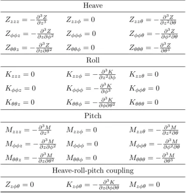
Tables 2-3 show the2nd_and3rd_{-order coefficients for}

each degree of freedom.

3.2 Hull-Wave Interaction Coefficients

Under the assumption of regular waves, the periodic wave passage along the hull produces cyclic variation in the restoring characteristics of the vessel. These

Table 2:2nd_{-order hydrostatic restoring coefficients}

Heave Roll Pitch

Zzz=−∂2_Z

∂z2 Kzz= 0 Mzz=−∂ 2_M

∂z2

Zzφ= 0 Kzφ=−_∂z∂φ∂2K Mzφ= 0 Zzθ=−∂2_Z

∂z∂θ Kzθ= 0 Mzθ=− ∂2_M

∂z∂θ

Zφφ =−∂2_Z

∂φ2 Kφφ= 0 Mφφ=−∂ 2_M

∂φ2

Zφθ= 0 Kφθ=−_∂φ∂θ∂2K Mφθ= 0 Zθθ=−∂_∂θ2Z2 Kθθ= 0 Mθθ=−

∂2_M

∂θ2

changes are taken into account by the 2nd _{and 3}rd

-order coefficients included in the nonlinear interactions

c_pos,sζ andc_pos,s2ζ+cpos,sζ2.

In order to determine the hull-wave interaction coef-ficients, the Froude-Krylov forces must be defined. The velocity potential for the undisturbed wave, as defined in (7), is given by

ϕI =Awg ωe e

kz_{sin(kxcosχ−kysinχ−ωet). (24)} Therefore, the1st _and2nd_{-order Froude-Krylov forces}

are:

FF K1

j (t) =ρ

Z Z _∂ϕI

∂t njdS (25)

FF K2

j (t) = 1 2ρ

Z Z

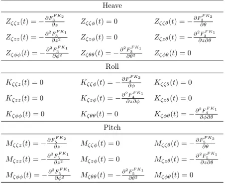
(∇ϕI· ∇ϕI)njdS (26) where n is the normal to the hull surface and j ad-dresses the specific mode for which the force is com-puted. The coefficients are then given by the formulas is Tables 4–5.

Due to the assumption of regular waves, the coeffi-cients can be described as a sum of a sine and a cosine term. For instance, the2nd_{-order term Kζφ(t), which}

is proportional to wave amplitude, can be written as Kζφ(t) =Aw(Kζφccosωet+Kζφssinωet) (27) whereKζφcandKζφs are constants.

Analogously, the3rd_{-order termsKζzφ(t)andKζφθ(t)}

are given by

Kζzφ(t) =Aw(Kζzφccosωet+Kζzφssinωet) (28) Kζφθ(t) =Aw(Kζφθccosωet+Kζφθssinωet). (29) These functions play an important role since they para-metrically excite the coupled system, being multiplied with, respectively,z(t)φ(t)andφ(t)θ(t).

The3rd_{-order termKζζφ(t), which is proportional to}

the wave amplitude squared, is given by Kζζφ(t) =A2w(Kζζφ0+Kζζφccos 2ωet

Table 3:3rd_{-order hydrostatic restoring coefficients}

Heave Zzzz=−∂3_Z

∂z3 Zzzφ= 0 Zzzθ=− ∂ 3_Z

∂z2_∂θ

Zφφz=− ∂3_Z

∂z∂φ2 Zφφφ= 0 Zφφθ=− ∂ 3_Z

∂φ2_∂θ

Zθθz=− ∂3_Z

∂z∂θ2 Zθθφ= 0 Zθθθ=−∂ 3_Z

∂θ3

Roll

Kzzz= 0 Kzzφ=−_∂z∂32K_∂φ Kzzθ = 0

Kφφz= 0 Kφφφ=−∂_∂φ3K3 Kφφθ = 0

Kθθz= 0 Kθθφ=−_∂φ∂θ∂3K2 Kθθθ= 0

Pitch Mzzz=−∂3_M

∂z3 Mzzφ= 0 Mzzθ=−∂ 3_M

∂z2_∂θ

Mφφz=−∂3_M

∂z∂φ2 Mφφφ= 0 Mφφθ=−

∂3_M

∂φ2_∂θ

Mθθz=−∂3_M

∂z∂θ2 Mθθφ= 0 Mθθθ=−

∂3_M

∂θ3

Heave-roll-pitch coupling

Zzφθ= 0 Kzφθ=−_{∂z∂φ∂θ}∂3K Mzφθ= 0

Table 4:2nd_{-order hydrostatic restoring coefficients due to wave passage}

Heave Roll Pitch

Zζz(t) =−∂F3F K1

∂z Kζz(t) = 0 Mζz(t) =− ∂FF K1

5

∂z Zζφ(t) = 0 Kζφ(t) =−∂F4F K1

∂φ Mζφ(t) = 0 Zζθ(t) =−∂F3F K1

∂θ Kζθ(t) = 0 Mζθ(t) =− ∂FF K1

5

∂θ

where it can be noticed the presence of a constant term plus a super-harmonic term of double the encounter frequency.

3.3 Nonlinear Restoring Forces and

Moments Redux

Rewriting the restoring forces and moments (11)–(15), according to the equations derived in this section gives:

• 1st_{-order body motions (c} pos,s)

Z_b(1)=Zzz+Zθθ

K_b(1)=Kφφ (31)

M_b(1)=Mzz+Mθθ

• 2nd_{-order body motions (c} pos,s2)

Zb(2)= 1 2(Zzzz

2_{+ 2Zzθzθ+Zφφφ}2_+Zθθθ2₎

K_b(2)=Kzφzφ+Kφθφθ (32)

M_b(2)=1 2(Mzzz

2_{+ 2Mzθzθ+Mφφφ}2_+Mθθθ2₎

• 2nd_{-order hull-wave interactions (c} pos,sζ)

Z_h/w(2) =Aw(Zζzcz+Zζθcθ) cosωet

+Aw(Zζzsz+Zζθsθ) sinωet

K_h/w(2) =Aw(Kζφccosωet+Kζφssinωet)φ (33) M_h/w(2) =Aw(Mζzcz+Mζθcθ) cosωet

+Aw(Mζzsz+Mζθsθ) sinωet

• 3rd_{-order body motions (c} pos,s3)

Z_b(3)= 1 6 Zzzzz

3_+Zθθθθ3_{+ 3Zzzθz}2_θ

+ 3Zφφzφ2z+ 3Zφφθφ2θ+ 3Zθθzθ2z

K_b(3)= 1

6 Kφφφφ

3_{+ 3Kzzφz}2_φ

+ 3Kθθφθ2_{φ+ 6Kzφθzφθ}

Table 5:3rd_{-order hydrostatic restoring coefficients due to wave passage}

Heave Zζζz(t) =−∂F

F K2 3

∂z Zζζφ(t) = 0 Zζζθ(t) =− ∂FF K2

3

∂θ

Zζzz(t) =−∂2F3F K1

∂z2 Zζzφ(t) = 0 Zζzθ(t) =−

∂2_FF K1 3

∂z∂θ

Zζφφ(t) =−∂2F

F K₁ 3

∂φ2 Zζθθ(t) =−

∂2_FF K₁ 3

∂θ2 Zζφθ(t) = 0

Roll Kζζz(t) = 0 Kζζφ(t) =−∂F

F K₂ 4

∂φ Kζζθ(t) = 0 Kζzz(t) = 0 Kζzφ(t) =−∂2F

F K1 4

∂z∂φ Kζzθ(t) = 0 Kζφφ(t) = 0 Kζθθ(t) = 0 Kζφθ(t) =−∂2F4F K1

∂φ∂θ

Pitch Mζζz(t) =−∂F5F K2

∂z Mζζφ(t) = 0 Mζζθ(t) =− ∂FF K2

5

∂θ

Mζzz(t) =−∂2F

F K₁ 5

∂z2 Mζzφ(t) = 0 Mζzθ(t) =−

∂2_FF K₁ 5

∂z∂θ

Mζφφ(t) =−∂2F

F K1 5

∂φ2 Mζθθ(t) =−

∂2_FF K1 5

∂θ2 Mζφθ(t) = 0

M_b(3) =1 6 Mzzzz

3_+Mθθθθ3_{+ 3Mzzθz}2_θ

+ 3Mφφzφ2_{z+ 3Mφφθφ}2_{θ+ 3Mθθzθ}2_z

• 3rd_{-order hull-wave interactions (c} pos,s2ζ

+c_pos,sζ2)

Z_h/w(3) =Zζzz(t)z2_{+Zζφφ(t)φ}2_{+Zζθθ(t)θ}2

+Zζzθ(t)zθ+Zζζz(t)z+Zζζθ(t)θ

K_h/w(3) =Kζzφ(t)zφ+Kζφθ(t)φθ

+Kζζφ(t)φ (35)

M_h/w(3) =Mζzz(t)z2+Mζφφ(t)φ2+Mζθθ(t)θ2

+Mζzθ(t)zθ+Mζζz(t)z+Mζζθ(t)θ

4 Matlab Implementation of the

Model

AMatlab/Simulinkmodel for the container ship model was developed for the purposes of simulating paramet-ric roll resonance, based on the model of Section 2.

For each time instant and system state, a function generates the instantaneous value of[˙sT_¨sT_]T_.

Numeri-cally integrating with an explicit Runge-Kutta method of order 4, with the fixed time step h= 1 s, the state [sTs_˙T_]T_{is calculated for any given time instant.}

The parameters used in the calculations are listed in Appendix A. While this was not done for the results

presented in this paper, for other encounter frequen-cies than the ones used in the experiments, interpola-tion can be applied to calculate approximate parameter values.

The code is part of the Marine Systems Simulator

(MSS, 2007).

5 Validation of the Model

Against Experimental Data

A comparison of the simulation and the experimental results can be seen in Figures 2–24.

The experiments were conducted with a 1:45 scale model ship in a towing tank. The experiments were done with varying forward speed, and wave frequency and height. This is summarized in Table 6. All data in the table and in the figures are in full scale.

The simulations were done with the code described in Section 4. All simulations were made ballistically. Initial conditions can be found in Table 7. Initial con-ditions not listed in the table (θ, z,˙ φ˙ andθ) were all˙ zero. The experiments were all assumed to start at t= 0.

Table 6: Experimental conditions

Exp. U [m/s] ω[rad/s] Aw[m] ωe [rad/s]

1172 5.4806 0.4640 2.5 0.5844

1173 5.4806 0.4425 2.5 0.5519

1174 5.4806 0.4764 2.5 0.6031

1175 5.4806 0.4530 2.5 0.5677

1176 5.4806 0.4893 2.5 0.6231

1177 5.4806 0.4640 1.5 0.5844

1178 5.4806 0.4699 1.5 0.5933

1179 5.4806 0.4583 1.5 0.5756

1180 5.4806 0.4640 3.5 0.5844

1181 5.4806 0.4425 3.5 0.5519

1182 5.4806 0.4893 3.5 0.6231

1183 5.4806 0.4530 3.5 0.5677

1184 5.7556 0.4640 2.5 0.5904

1185 6.0240 0.4640 2.5 0.5963

1186 6.2990 0.4640 2.5 0.6023

1187 6.5740 0.4640 2.5 0.6084

1188 7.1241 0.4640 2.5 0.6204

1189 7.6675 0.4640 2.5 0.6324

1190 7.3991 0.4640 2.5 0.6265

1191 5.2056 0.4640 2.5 0.5783

1192 4.6555 0.4640 2.5 0.5662

1193 4.9305 0.4640 2.5 0.5723

Table 7: Simulation initial conditions

Exp. z0 [m] φ0 [rad]

1172 0.0250 3.4907e-3

1173 0.0500 3.4907e-2

1174 0.0500 3.4907e-5

1175 0.0500 1.7453e-4

1176 0.0500 1.7453e-5

1177 0.0500 1.3963e-2

1178 0.0500 8.7266e-3

1179 0.0500 3.4907e-2

1180 0.0500 8.7266e-5

1181 0.0500 3.4907e-2

1182 0.0500 1.7453e-5

1183 0.0500 8.7266e-6

1184 0.0500 1.7453e-3

1185 0.0500 5.2360e-4

1186 0.0500 8.7266e-5

1187 0.0500 5.2360e-4

1188 0.0500 5.2360e-4

1189 0.0500 2.4435e-3

1190 0.0500 1.7453e-4

1191 0.0500 3.4907e-3

1192 0.0500 3.4907e-2

1193 0.0500 1.7453e-3

Table 8: Simulation results

Exp. Aw ω ωe/ω0 max|φ_sim| max|φ_exp| Error %

1179 1.5 0.4583 1.9337 2.0000 0.4729 323

1177 1.5 0.4640 1.9633 8.0982 17.1140 -53

1178 1.5 0.4699 1.9932 12.0995 22.5530 -46

1173 2.5 0.4425 1.8541 2.0000 0.7142 180

1175 2.5 0.4530 1.9072 0.6084 0.7215 -16

1192 2.5 0.4640 1.9021 9.7799 0.8944 993

1193 2.5 0.4640 1.9226 11.8080 1.8932 524

1191 2.5 0.4640 1.9428 13.5465 21.7800 -38

1172 2.5 0.4640 1.9633 15.1622 23.9270 -37

1184 2.5 0.4640 1.9834 16.5792 22.7810 -27

1185 2.5 0.4640 2.0032 17.8812 20.8780 -14

1186 2.5 0.4640 2.0234 19.2712 21.5640 -11

1187 2.5 0.4640 2.0439 20.4611 20.4990 0

1188 2.5 0.4640 2.0842 22.4097 22.7190 -1

1190 2.5 0.4640 2.1047 23.4472 1.4291 1541

1189 2.5 0.4640 2.1245 24.2884 1.4368 1590

1174 2.5 0.4764 2.0261 21.4924 26.6960 -19

1176 2.5 0.4893 2.0933 26.7459 1.2581 2026

1181 3.5 0.4425 1.8541 2.0000 2.0352 -2

1183 3.5 0.4530 1.9072 11.0859 8.9410 24

1180 3.5 0.4640 1.9633 18.8898 23.9530 -21

column is maximum roll amplitude for the simulations (max|φsim|). The sixth is maximum roll amplitude for

the experiments (max|φexp|). The seventh and final

column is the percentage error given by 100max|φsim| −max|φexp|

max|φexp|

,

rounded to integer value. Note that most of the exper-iments were stopped before the final steady-state roll angle could be achieved due to fear of vessel capsizing. Figures 2–22 show heave, roll and pitch as functions of time, both experimental and simulated.

0 200 400 600 800 1000 −2

−1 0 1 2

z [m]

0 200 400 600 800 1000 −30

−15 0 15 30

φ

[deg]

0 200 400 600 800 1000 −3

−1.5 0 1.5 3

θ

[deg]

time [s]

Figure 2: Exp. 1172. Exp. dashed red, sim. solid blue.

0 200 400 600 800 1000 −2

−1 0 1 2

z [m]

0 200 400 600 800 1000 −30

−15 0 15 30

φ

[deg]

0 200 400 600 800 1000 −3

−1.5 0 1.5 3

θ

[deg]

time [s]

Figure 3: Exp. 1173. Exp. dashed red, sim. solid blue.

In Figure 24, we can see the maximum roll angle achieved in the simulations and experiments for cer-tain conditions, plotted against the ratio of encounter frequency to natural roll frequency (ωe/ω0). The data

in the figure is all for Aw = 2.5 m, and ω = 0.4640 rad/s.

0 200 400 600 800 1000 −2

−1 0 1 2

z [m]

0 200 400 600 800 1000 −30

−15 0 15 30

φ

[deg]

0 200 400 600 800 1000 −3

−1.5 0 1.5 3

θ

[deg]

time [s]

Figure 4: Exp. 1174. Exp. dashed red, sim. solid blue.

0 200 400 600 800 1000 −2

−1 0 1 2

z [m]

0 200 400 600 800 1000 −30

−15 0 15 30

φ

[deg]

0 200 400 600 800 1000 −3

−1.5 0 1.5 3

θ

[deg]

time [s]

Figure 5: Exp. 1175. Exp. dashed red, sim. solid blue.

0 200 400 600 800 1000 −2

−1 0 1 2

z [m]

0 200 400 600 800 1000 −30

−15 0 15 30

φ

[deg]

0 200 400 600 800 1000 −3

−1.5 0 1.5 3

θ

[deg]

time [s]

0 200 400 600 800 1000 −2 −1 0 1 2 z [m]

0 200 400 600 800 1000 −30 −15 0 15 30 φ [deg]

0 200 400 600 800 1000 −3 −1.5 0 1.5 3 θ [deg] time [s]

Figure 7: Exp. 1177. Exp. dashed red, sim. solid blue.

0 200 400 600 800 1000 −2 −1 0 1 2 z [m]

0 200 400 600 800 1000 −30 −15 0 15 30 φ [deg]

0 200 400 600 800 1000 −3 −1.5 0 1.5 3 θ [deg] time [s]

Figure 8: Exp. 1180. Exp. dashed red, sim. solid blue.

0 200 400 600 800 1000 −2 −1 0 1 2 z [m]

0 200 400 600 800 1000 −30 −15 0 15 30 φ [deg]

0 200 400 600 800 1000 −3 −1.5 0 1.5 3 θ [deg] time [s]

Figure 9: Exp. 1178. Exp. dashed red, sim. solid blue.

0 200 400 600 800 1000 −2 −1 0 1 2 z [m]

0 200 400 600 800 1000 −30 −15 0 15 30 φ [deg]

0 200 400 600 800 1000 −3 −1.5 0 1.5 3 θ [deg] time [s]

Figure 10: Exp. 1181. Exp. dashed red, sim. solid blue.

0 200 400 600 800 1000 −2 −1 0 1 2 z [m]

0 200 400 600 800 1000 −30 −15 0 15 30 φ [deg]

0 200 400 600 800 1000 −3 −1.5 0 1.5 3 θ [deg] time [s]

Figure 11: Exp. 1179. Exp. dashed red, sim. solid blue.

0 200 400 600 800 1000 −2 −1 0 1 2 z [m]

0 200 400 600 800 1000 −30 −15 0 15 30 φ [deg]

0 200 400 600 800 1000 −3 −1.5 0 1.5 3 θ [deg] time [s]

0 200 400 600 800 1000 −2 −1 0 1 2 z [m]

0 200 400 600 800 1000 −30 −15 0 15 30 φ [deg]

0 200 400 600 800 1000 −3 −1.5 0 1.5 3 θ [deg] time [s]

Figure 13: Exp. 1183. Exp. dashed red, sim. solid blue.

0 200 400 600 800 1000 −2 −1 0 1 2 z [m]

0 200 400 600 800 1000 −30 −15 0 15 30 φ [deg]

0 200 400 600 800 1000 −3 −1.5 0 1.5 3 θ [deg] time [s]

Figure 14: Exp. 1186. Exp. dashed red, sim. solid blue.

0 200 400 600 800 1000 −2 −1 0 1 2 z [m]

0 200 400 600 800 1000 −30 −15 0 15 30 φ [deg]

0 200 400 600 800 1000 −3 −1.5 0 1.5 3 θ [deg] time [s]

Figure 15: Exp. 1184. Exp. dashed red, sim. solid blue.

0 200 400 600 800 1000 −2 −1 0 1 2 z [m]

0 200 400 600 800 1000 −30 −15 0 15 30 φ [deg]

0 200 400 600 800 1000 −3 −1.5 0 1.5 3 θ [deg] time [s]

Figure 16: Exp. 1187. Exp. dashed red, sim. solid blue.

0 200 400 600 800 1000 −2 −1 0 1 2 z [m]

0 200 400 600 800 1000 −30 −15 0 15 30 φ [deg]

0 200 400 600 800 1000 −3 −1.5 0 1.5 3 θ [deg] time [s]

Figure 17: Exp. 1185. Exp. dashed red, sim. solid blue.

0 200 400 600 800 1000 −2 −1 0 1 2 z [m]

0 200 400 600 800 1000 −30 −15 0 15 30 φ [deg]

0 200 400 600 800 1000 −3 −1.5 0 1.5 3 θ [deg] time [s]

0 200 400 600 800 1000 −2

−1 0 1 2

z [m]

0 200 400 600 800 1000 −30

−15 0 15 30

φ

[deg]

0 200 400 600 800 1000 −3

−1.5 0 1.5 3

θ

[deg]

time [s]

Figure 19: Exp. 1189. Exp. dashed red, sim. solid blue.

0 200 400 600 800 1000 −2

−1 0 1 2

z [m]

0 200 400 600 800 1000 −30

−15 0 15 30

φ

[deg]

0 200 400 600 800 1000 −3

−1.5 0 1.5 3

θ

[deg]

time [s]

Figure 20: Exp. 1192. Exp. dashed red, sim. solid blue.

0 200 400 600 800 1000 −2

−1 0 1 2

z [m]

0 200 400 600 800 1000 −30

−15 0 15 30

φ

[deg]

0 200 400 600 800 1000 −3

−1.5 0 1.5 3

θ

[deg]

time [s]

Figure 21: Exp. 1190. Exp. dashed red, sim. solid blue.

0 200 400 600 800 1000 −2

−1 0 1 2

z [m]

0 200 400 600 800 1000 −30

−15 0 15 30

φ

[deg]

0 200 400 600 800 1000 −3

−1.5 0 1.5 3

θ

[deg]

time [s]

Figure 22: Exp. 1193. Exp. dashed red, sim. solid blue.

0 200 400 600 800 1000 −2

−1 0 1 2

z [m]

0 200 400 600 800 1000 −30

−15 0 15 30

φ

[deg]

0 200 400 600 800 1000 −3

−1.5 0 1.5 3

θ

[deg]

time [s]

Figure 23: Exp. 1191. Exp. dashed red, sim. solid blue.

1.95 2 2.05 2.1

0 5 10 15 20 25 30 35

ω_e/ω₀

max(|

φ

|) [deg]

Figure 24: Max. roll angle vsωe/ω0 forAw= 2.5

6 Analysis of the Model Based

Upon the Validation Results

The3rd_{-order model developed for the281mlong}

con-tainer ship shows high capabilities in reproducing the vertical and transversal dynamics of the vessel under parametric resonance conditions, as shown by the com-parison of the experimental results (Figures 2–24).

Considering the 13 experiments where parametric resonance did occur, the implemented model performs well: starting from similar initial conditions and being subjected to the same excitation forces used during the experiments, the model develops parametric resonance within the same time frame as the 1:45 scale model ship in most of the cases.

The most obvious differences between the simulation and the experimental results consists of the amplitude of the oscillations. In all the experiments where para-metric resonance occurred, the peak value of the roll oscillations is higher than the saturation level at which the model settles. Although the model has a general tendency to underestimate the peak value of the roll motion, the gap is relatively small in most cases.

Considering the 9 experiments where parametric roll did not occur, the model produced 5 false positive cases developing resonant motion. In order to understand this disagreement between model behavior and experi-mental results, the tuning factorωe/ω0 must be taken

into consideration. In fact all the 5 false-positive cases occur with a tuning factor close to the limits of the first instability region of the Hill-Mathieu Equation (ωe≈2ω0), as shown in Figure 24. Looking at the peak

value of the roll oscillations (Figure 24 and Table 8), it is seen that the largest differences are in the region of high tunings (ωe

ω0 >2.1) for which the model predicts

large roll motion whereas the experiments showed no amplification. It seems obvious that when the experi-mental conditions are close to the limits of stability the model does not match exactly the frequency at which the abrupt variation in roll motion take place.

The errors indicated in tests 1173, 1179 and 1181 have no real physical meaning, since the initial condi-tion of 2 degrees was chosen arbitrarily high in order to indicate a decaying motion.

For all 22 experiments, heave and pitch dynamics have shown relatively good agreement with the exper-iments. In all the test runs the two modes oscillates at the excitation frequency, matching the experimen-tal records. The amplitude of the oscillations is close to that of the experimental values.

7 Conclusions

A Matlab/Simulink benchmark for the simulation of parametric roll resonance for a large container ship has been implemented and validated against experimental results. The implementation reflects the coupled 3rd

-order nonlinear model for parametric roll first intro-duced by Neves and Rodríguez (2005).

The mathematical model for the container ship at hand, already presented in Rodríguez et al. (2007), has been reviewed, illustrating in details the ship dynamics that has been taken into account. 1st_,2nd_and3rd_-order

contributions have been described and analytical for-mulas of all the couplings coefficients due to heave, roll, pitch, and wave motion have been given. Furthermore, numerical values of all coefficients are computed based upon the hull geometry and wave characteristics.

The benchmark has been tested on a set of 22 differ-ent conditions, which have been chosen to match the experimental conditions. Each test run differs from the previous for at least the value of one parameter among ship speed, wave frequency, and wave height. The heave and pitch dynamics described by the model are in good accordance with the experimental results. The model seems to reproduce the pitch motion slightly better, catching the right amplitude in most of the cases.

The results obtained in roll have shown good agree-ment with the records of the experiagree-ments. In particu-lar, the model agrees with the experiments in all the cases where parametric roll occurred, although the am-plitude of the roll oscillations does not quite reach the experimental peak value in most cases.

For the experiments where there was no parametric roll, then the model produces false positives in about 50% of the cases. This disagreement between the sim-ulation and the experimental results is believed to be related to the specific values of the tuning factorωe/ω0

which were too close to the limits of the first instability region of the Hill-Mathieu Equation. In these cases, it is very difficult to get the correct response with ballistic simulations.

The availability of this benchmark offers a wide range of opportunities for development of new model-based control strategies for counteracting or preventing para-metric roll resonance.

A Tables of Coefficients

The parameters can be found in Tables 9–16. All num-bers are given in the kg-m-s (SI) system. Only non-zero numbers are listed.

hydro-dynamic damping parameters, while Table 12 contains the body motion parameters. Table 13 contains the wave motion parameters for heave. Table 14 contains the wave motion parameters for roll. Table 15 contains the wave motion parameters for pitch. Table 16 con-tains the external wave excitation parameters. Note thatα3 andα5 are given in radians.

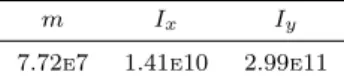
Table 9: Rigid body inertia

m I_x I_y

7.72e7 1.41e10 2.99e11

Table 12: Restoring force (motions)

Heave Roll Pitch

Z_{z = 7.9882e7} K_{φ = 1.4340e9} M_{z = 7.6622e8} Z_{θ = 7.6622e8} K_{φφφ= 1.7844e10} M_{θ = 4.1365e11} Z_zz =-3.0014e6 K_zφ =-8.4268e7 M_zz =-2.4985e8

Z_zθ =-2.4986e8 K_φθ =-1.4090e10 M_zθ =-4.9230e10

Z_{zφ =-2.9468e8} K_{zzφ= 7.9738e7} M_{zφ =-2.0614e10} Z_{θθ =-4.9230e10} K_{φθθ= 1.5400e11} M_{θθ =-4.8730e12} Z_{zφφ= 2.8817e8} M_{zφφ= 2.7052e10} Z_φφθ= 2.7052e10 M_φφθ= 4.1064e12

Z_θθθ= 1.5324e9 M_θθθ= 8.5664e11

Table 14: Restoring force roll (wave)

ω K_ζφc K_ζφs

0.4425 -2.0159e8 5.0131e7

0.4530 -2.2088e8 3.9835e7

0.4583 -2.2955e8 2.9048e7

0.4640 -2.3800e8 1.7097e7 0.4699 -2.4571e8 -1.4401e7

0.4764 -2.5289e8 -2.0107e7

0.4893 -2.6271e8 -5.1159e7

Acknowledgements

The authors would like to thank MARINTEK for hav-ing provided the experimental facilities and the finan-cial support. Many thanks are due to Dr. Ingo Drum-men for having collected the experiDrum-mental data. This work was partially supported in Brazil by CNPq within the STAB project (Nonlinear Stability of Ships), by LabOceano-COPPE/UFRJ and CAPES, and in Nor-way by CESOS (Centre of Excellence for Ships and Ocean Structures).

References

Bulian, G. Development of analytical nonlinear models for parametric roll and hydrostatic restoring

varia-Table 16: External wave forces

ω_e F¯₃ α₃ F¯₅ α₅

0.5519 1.1189e7 -0.0000 2.9506e9 4.8904

0.5662 0.5271e7 -0.2025 2.6579e9 4.8730

0.5677 0.8123e7 -0.0750 2.8144e9 4.8817

0.5723 0.5222e7 -0.2147 2.6552e9 4.8730

0.5756 0.6653e7 -0.1361 2.7384e9 4.8764

0.5783 0.5175e7 -0.2269 2.6525e9 4.8712

0.5844 0.5130e7 -0.2391 2.6500e9 4.8695

0.5904 0.5086e7 -0.2496 2.6475e9 4.8695

0.5933 0.3709e7 -0.4189 2.5538e9 4.8642

0.5963 0.5157e7 -0.2478 2.6549e9 4.8712

0.6023 0.5138e7 -0.2548 2.6545e9 4.8695 0.6031 0.2489e7 -0.8186 2.4424e9 4.8573

0.6084 0.5105e7 -0.2653 2.6528e9 4.8695

0.6204 0.4957e7 -0.2950 2.6423e9 4.8660

0.6231 0.2816e7 -2.1398 2.1973e9 4.8381

0.6265 0.4886e7 -0.3107 2.6373e9 4.8642 0.6324 0.4838e7 -0.3229 2.6341e9 4.8642

tions in regular and irregular waves. Ph.D. thesis, Università degli Studi di Trieste, 2006.

Carmel, S. M. Study of parametric rolling event on a panamax container vessel. Journal of the Trans-portation Research Board, 2006. 1963:56–63. France, W. N., Levadou, M., Treakle, T. W., Paulling,

J. R., Michel, R. K., and Moore, C. An investiga-tion of head-sea parametric rolling and its influence on container lashing systems. In SNAME Annual Meeting. 2001 .

Francescutto, A. An experimental investigation of parametric rolling in head waves.Journal of Offshore Mechanics and Arctic Engineering, 2001. 123:65–69. Francescutto, A. and Bulian, G. Nonlinear and stochastic aspects of parametric rolling modelling. InProc. of the 6th International Ship Stability Work-shop. 2002 .

Himeno, Y. Prediction of ship roll damping - state of the art. Technical report, Department of Naval Ar-chitecture and Marine Engineering, The University of Michigan, 1981.

Jensen, J. J. Effcient estimation of extreme non-linear roll motions using the first-order reliability method (FORM_{). Marine Science and Technology, 2007.}

12(4):191–202.

MSS. Marine S_ystems S_{imulator - Matlab/Simulink} T_{oolbox. <www.marinecontrol.org>, 2007.}

Ac-cessed November 30.

Table 10: Added mass

ω_e Z_z¨ Z_¨

θ Kφ¨ Mz¨ Mθ¨ 0.5519 8.4377e7 5.2986e8 2.17e9 2.2140e9 4.3227e11

0.5662 8.3596e7 6.8658e8 2.17e9 2.0263e9 4.2368e11

0.5677 8.3515e7 5.7142e8 2.17e9 2.1383e9 4.2519e11

0.5723 8.3266e7 6.5957e8 2.17e9 2.0402e9 4.2169e11

0.5756 8.3077e7 5.9056e8 2.17e9 2.1017e9 4.2161e11

0.5783 8.2935e7 6.3403e8 2.17e9 2.0526e9 4.1972e11

0.5844 8.2604e7 6.0987e8 2.17e9 2.0637e9 4.1775e11

0.5904 8.2273e7 5.8702e8 2.17e9 2.0734e9 4.1579e11

0.5933 8.2112e7 6.2852e8 2.17e9 2.0255e9 4.1376e11 0.5963 8.1955e7 5.6623e8 2.17e9 2.0816e9 4.1392e11

0.6023 8.0509e7 5.2790e8 2.17e9 2.0821e9 4.0685e11

0.6031 8.1568e7 6.4758e8 2.17e9 1.9849e9 4.0935e11

0.6084 8.0003e7 5.0546e8 2.17e9 2.0875e9 4.0410e11

0.6204 7.9811e7 4.7712e8 2.17e9 2.1003e9 4.0240e11 0.6231 8.0481e7 6.8112e8 2.17e9 1.9082e9 4.0059e11

0.6265 7.9714e7 4.6449e8 2.17e9 2.1051e9 4.0155e11

0.6324 7.9491e7 4.5092e8 2.17e9 2.1082e9 4.0014e11

Table 11: Hydrodynamic damping

ω_e Z_z˙ Z_˙

θ Kφ˙ Kφ˙|φ˙| Mz˙ Mθ˙ 0.5519 4.6790e7 1.1900e9 3.1951e8 2.9939e8 2.6485e8 2.7431e11

0.5662 4.6121e7 1.1146e9 3.0467e8 3.7433e8 3.3617e8 2.7151e11

0.5677 4.6051e7 1.1830e9 3.1951e8 2.9939e8 2.6733e8 2.7254e11

0.5723 4.5838e7 1.1351e9 3.0962e8 3.4696e8 3.1392e8 2.7124e11

0.5756 4.5676e7 1.1795e9 3.1951e8 2.9939e8 2.6859e8 2.7166e11

0.5783 4.5554e7 1.1555e9 3.1456e8 3.2205e8 2.9184e8 2.7097e11

0.5844 4.5271e7 1.1757e9 3.1951e8 2.9939e8 2.6995e8 2.7071e11

0.5904 4.4987e7 1.1956e9 3.2445e8 2.7877e8 2.4824e8 2.7045e11

0.5933 4.4849e7 1.1717e9 3.1951e8 2.9939e8 2.7136e8 2.6973e11

0.5963 4.4714e7 1.2147e9 3.2921e8 2.6067e8 2.2754e8 2.7020e11

0.6023 4.4749e7 1.2312e9 3.3415e8 2.4348e8 2.1714e8 2.7166e11

0.6031 4.4383e7 1.1673e9 3.1951e8 2.9939e8 2.7292e8 2.6866e11 0.6084 4.4524e7 1.2498e9 3.3910e8 2.2779e8 1.9803e8 2.7167e11

0.6204 4.3839e7 1.2892e9 3.4898e8 2.0031e8 1.5198e8 2.7044e11

0.6231 4.3451e7 1.1585e9 3.1951e8 2.9939e8 2.7605e8 2.6654e11

0.6265 4.3497e7 1.3088e9 3.5393e8 1.8826e8 1.2903e8 2.6982e11

0.6324 4.3198e7 1.3274e9 3.5878e8 1.7741e8 1.0805e8 2.6943e11

Table 13: Restoring force heave (wave)

ω Z_ζzc Z_ζzs Z_ζθc Z_ζθs Z_ζφφc Z_ζφφs

0.4425 -2.3750e6 6.6977e5 -2.4465e8 2.9599e8 8.1275e7 -5.4920e7 0.4530 -2.5435e6 3.2979e5 -2.5538e8 2.5518e8 9.8517e7 -3.6843e7

0.4583 -2.6145e6 2.0307e5 -2.5920e8 1.3333e8 9.1601e7 -3.3192e7

0.4640 -2.6795e6 1.6335e5 -2.6201e8 1.0901e8 9.4449e7 -2.0234e7

0.4699 -2.7334e6 -1.1570e5 -2.6345e8 1.8304e8 10.6854e7 -1.7722e7

0.4764 -2.7763e6 -2.5049e5 -2.6320e8 1.5364e8 10.8827e7 -0.6161e7

0.4893 -2.8063e6 -6.1952e5 -2.5674e8 -0.9361e8 10.0490e7 1.3270e7

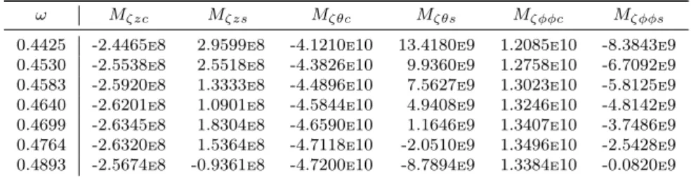
Table 15: Restoring force pitch (wave)

ω M_ζzc M_ζzs M_ζθc M_ζθs M_ζφφc M_ζφφs

0.4425 -2.4465e8 2.9599e8 -4.1210e10 13.4180e9 1.2085e10 -8.3843e9

0.4530 -2.5538e8 2.5518e8 -4.3826e10 9.9360e9 1.2758e10 -6.7092e9

0.4583 -2.5920e8 1.3333e8 -4.4896e10 7.5627e9 1.3023e10 -5.8125e9

0.4640 -2.6201e8 1.0901e8 -4.5844e10 4.9408e9 1.3246e10 -4.8142e9

0.4699 -2.6345e8 1.8304e8 -4.6590e10 1.1646e9 1.3407e10 -3.7486e9

0.4764 -2.6320e8 1.5364e8 -4.7118e10 -2.0510e9 1.3496e10 -2.5428e9

waves. InProc. of the 6th International Ship Stabil-ity Workshop. 2002 .

Neves, M. A. S. and Rodríguez, C. A. A coupled third order model of roll parametric resonance. Mar-itime Transportation and Exploitation of Ocean and Coastal Resources, 2005.

Neves, M. A. S. and Rodríguez, C. A. An investiga-tion on roll parametric resonance in regular waves. InProc. of the 9th International Conference on Sta-bility of Ships and Ocean Vehicles. 2006a .

Neves, M. A. S. and Rodríguez, C. A. On unstable ship motions resulting from strong non-linear coupling.

Ocean Engineering, 2006b. 33:1853–1883.

Newman, J. N. Marine Hydrodynamics. The MIT Press, 1977.

Nielsen, J. K., Pedersen, N. H., Michelsen, J., Nielsen, U. D., Baatrup, J., Jensen, J. J., and Petersen, E. S. SeaS_{ense - real-time onboard decision support. In}

World Maritime Technology Conference. 2006 .

Palmquist, M. and Nygren, C. Recording of head-sea parametric rolling on a PCTC_{. Technical report,}

International Maritime Organization, 2004. Perez, T. Ship Motion Control. Springer, 2005. Rodríguez, C. A., Holden, C., Perez, T., Drummen,

I., Neves, M. A. S., and Fossen, T. I. Validation of a container ship model for parametric rolling. In

Proc. of the 9th International Ship Stability Work-shop. 2007 .

Salvesen, N., Tuck, O. E., and Faltinsen, O. Ship mo-tions and sea loads. Transactions of SNAME, 1970. 78:250–287.

Shin, Y. S., Belenky, V. L., Paulling, J. R., Weems, K. M., and Lin, W. M. Criteria for parametric roll of large containeships in longitudinal seas. Transac-tions of SNAME, 2004. 112.

Tondl, A., Ruijgrok, T., Verhulst, F., and Nabergoj, R.