A NEW METHOD TO DETECT REGIONS ENDANGERED BY HIGH WIND SPEEDS
P. Fischer *, S. Ehrensperger, T. Krauß
Remote Sensing Technology Istitute, German Aerospace Center (DLR), Münchener Str. 20, 82234 Wessling, Germany – (Peter.Fischer, Thomas.Krauss)@dlr.de, [email protected]
Commission VIII, WG VIII/1
KEY WORDS: Non-Parametric Regression, Boosted Regression Trees, Wind Speeds, Spatial Predictions
ABSTRACT:
In this study we evaluate whether the methodology of Boosted Regression Trees (BRT) suits for accurately predicting maximum wind speeds. As predictors a broad set of parameters derived from a Digital Elevation Model (DEM) acquired within the Shuttle Radar Topography Mission (SRTM) is used. The derived parameters describe the surface by means of quantities (e.g. slope, aspect) and quality (landform classification). Furthermore land cover data from the CORINE dataset is added. The response variable is maximum wind speed, measurements are provided by a network of weather stations. The area of interest is Switzerland, a country which suits perfectly for this study because of its highly dynamic orography and various landforms.
1. INTRODUCTION
Storms are one of the major natural hazards, being responsible for about 80% of the 415 Billion US Dollar which insurance companies had to pay between 1950 and 2009 to meet their obligations (MunichRE). The damage potential for single events is extremely huge. Besides of the increasing number and denseness of ensured entities also changing weather pattern induced through the global warming of the atmosphere sign responsible for the rise in damages caused by storms.
The accurate description of wind fields, their movement patterns over ground and the corresponding wind speeds, is still a challenging task. Various reasons contribute to this situation. First, wind flux responds very sensible on the roughness of surfaces (e.g. changing vegetation, buildings), this variable is under permanent change. Additional variation comes from orography (e.g. hills, mountains, valleys, canyons) causing suspension of air masses, turbulences and channelling effects. Such phenomena already occur on a small scale, meteorological measurement nets are mostly to coarse to record such local phenomena.
In our study we focus on the estimation of maximum wind speeds based on remote sensing data. As in a previous study, we use a DEM and derived parameters of the DEM to give a detailed description of earth surface. We extend the number of DEM based parameters adding surface roughness and surface ruggedness to the predictors. As a further step we add land cover data to the predictors, namely the CORINE (Co-ordination of Information on the Environment) Land Cover (CLC) dataset provided and maintained by the European Environmental Agency (EEA).
As methodologic approach we use BRT, a non-parametric regression technique which is applied in a broad range of spatial applications during the last decade.
2. PREDICTORS AND RESPONSE
To reach the goal of predicting max. wind speeds, we need to resolve the linkage between the three dimensional earth surface, its describing parameters and the wind speeds which can be measured for locations. The formulation of this problem is �=�̂(�1,�2, … ,��), where x are the predictors derived from remote sensing data, and y is the measured response. �̂ is the
unknown functional dependency, which needs to be resolved. The predictors are mainly divided into two groups,
1. DEM and DEM based parameters 2. Land Cover
Both data sources will be introduced in the following subsections. The response is given as gust wind speed, the detailed description of this parameter is given at the end of this section.
2.1 DEM and DEM based parameters
We use a DEM recorded by the National Aeronautics and Space Administration's (NASA) Shuttle Radar Topography Mission (SRTM), data access is provided via a website maintained by the U.S. Geological Survey. A detailed description of the SRTM data is given in (Farr et al., 2007). We derived a broad set of descriptive parameters from this dataset, an overview is given in table 1.
Parameter Data class
Slope Numeric
Aspect Numeric
Planform/Profile Curvature Numeric Terrain Ruggedness Index Numeric Terrain Roughness Index Numeric Topographic Position Index Categorical
TOPEX Numeric
Table 1. DEM based parameters
A detailed description of most of the parameters is given in (Li et al., 2005), the methodology of landform classification is inspired by (Weiss, 2001), the TOPEX score is derived from (Chapman, 2000).
2.2 CORINE Land Cover
were used. The dataset gives detailed information about Land Cover for 44 classes with a thematic accuracy of > 85%. A detailed description of the data, the current status of the project and future steps is given by (Büttner, 2014).
2.3 Gust Wind Speeds
As a rule of thumb, the higher the wind speed the higher the damage costs are. To target this, we decided to focus on gust wind speeds rather than mean wind speeds. The Swiss Meteorological Service Meteo Swiss maintains a network of 160 stations spread over the country, collecting gust wind speeds with a daily granularity.
We obtained this dataset and took the 98. Percentile of each station as input for our model, as this is known as a suitable descriptor of damage functions of storm events (Klawa and Ulbricht, 2003).
3. ALGORITHM
BRT is a simple yet powerful method from the statistical learning community. The algorithm is an ensemble method, wherein several single models are combined in an additive way to build up the final model. One of the core strength of this statistical method is the ability to handle numeric data (e.g. Height in metres, Slope in degrees) and categorical data (e.g. Landform, Land Cover). An in-depth description of the algorithm and its components is given in (Hastie et al, 2014), for completeness we give an overview about the main components and tuning parameters in the following three subsections.
3.1 Regression Trees
The core component of the algorithm are regression trees. Trees are a combination of decision rules derived from a set of training data. This set contains � observations, each observation consists of a response � and � independent predictors ��. The regression tree models the dependency between predictors and response, e.g.
�=�̂(�1,�2, … ,��).
The building of the tree is an iterative process. During this process the predictor space is divided into � regions ��. At each iteration the algorithm tries to minimize the model error targeting a given error function, e.g. sum of squared error ∑��=1(��− �̂(��))2. The modelled response value �� of a region is then simply the average response of all responses covered by this region, e.g.
��=���(�|� ∈ ��).
At initialization the tree consists solely of a root node. In each iteration a new decision rule is derived to separate predictor space, the rule is described by a split value � and the subgroup of target predictors �. The rule can then be written as
�1(�,�) = {�|��≤ �} and �2(�,�) = {�|��>�},
which yields a binary split point. The determination of the (�,�) tuple is done by minimizing the overall error of both branches of the decision node, which is written as
min
�,� �min�1 � (� − �1)
2 �∈�1(�,�)
+ min
�2 � (� − �2)
2 �∈�2(�,�)
�
The decision node leads now to two leafs. In the following iteration one of the two leafs will also become a decision node, this procedure continues until a given stopping criterion is met, e.g. max. number of leafs, max. tree depth, min. number of samples per leaf or a reduction of the model error below a given threshold.
3.2 Boosting
Boosting is a possibility to extend the basic Regression Tree algorithm. Instead of growing one deep tree which aims to depict the in most cases quite complex interactions between the set of predictors, a big number of trees is sequentially build, each new tree aiming to minimize the residuals of its precursor. This strategy is widely known as Gradient Boosting.
After the building of the first regression tree, the Loss function � of the regression tree model �̂ itself can be written as
���̂�= � �(��,�̂(��)
�
�=1
Gradient Boosting aims now to minimize the overall loss of the model by adding iteratively new trees to the model.
3.3 Regularization
Several options are available to avoid overfitting during the model building process. Tree complexity addresses the depth of a tree. A tree with a depth of one is just the root node with two terminal nodes, often revered as single decision stumps. The deeper a tree grows, the more interaction between variables is included. As boosting iteratively adds a new tree to an existing ensemble of trees, the single trees don't necessarily need to grow deep.
The total number of trees and the learning rate are two further parameters strongly related to each other. In general each tree aims to minimize the residuals of its precursor tree. The contribution of the first trees in minimizing the overall model error is big, whilst in later iterations the total error is just slightly reduced by new trees and the model tends to overfit. Learning rate is therefore a parameter to lower the influence of newly added trees to an existing model. The goal is to find the perfect number of trees which reduce the error most without overfitting the model to the given training dataset.
4. EXPERIMENT
The main task in this work was finding a model that fits the data of the wind measurements in a way that is strictly enough to make predictions about unseen data, but also loose enough to not be biased by the underlying data. This is achieved by extracting the function hidden in the data using non-parametric regression methods, namely BRT. Therefore we use the derived parameters of a DEM and also the CLC dataset to get a description of the surface forming the movement of wind. These data are used as features to explain the relationship between terrain and airflow.
4.1 Description of Experiment
values. The test set is used to evaluate the model after it is trained. By this way it is possible to evaluate the predicted outcomes using real world data. The split is made in a ratio of 70% training set and 30% test set.
The values chosen for the evaluation are Mean Squared Error (MSE), Root Mean Squared Error (RMSE) and the coefficient of determination r². Because of the small overall dataset the method of cross-validation is used. It randomly chooses different distributions of the train and test set and calculates the evaluation values for every one of these distributions. In the end it delivers an average value for all random splits. This process precludes the possibility of a random bias in the training and test set.
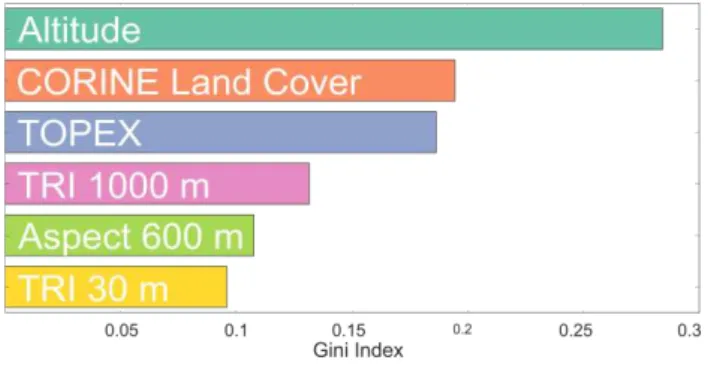
A brute force method to train the model with all possible combinations of regularization parameters within given intervals is used to check which are the best regularization parameters. Based on these parameters an elementary model is built to extract the most important features. The feature importance is determined by the Gini-index. This index uses the contribution to the decisions made over the whole BRT giving values between 1 and 0 for each feature.
Then the parameters are further tuned to control the complexity of the model, with the goal to find a balanced setup between a too loose and a too strict model. Also, the combination of features is further investigated by using an iterative approach while checking the evaluation values. For the final model a specific train and test set split is chosen which represents the values of the cross-validation results. This model is then used to create the wind speed map of Switzerland.
4.2 Description of Results
The indicators providing a quantitative validation of the results are the RMSE of 3.42 and r² of 0.58. The selected features and their importance are shown in Figure 1.
Figure 1: Feature importance
The deviance plot is illustrated in Figure 2. It shows the value of the loss function for the train and test set in dependence of the boosting iterations.
Figure 2: Deviance Plot
The learning curve is shown in Figure 3. It indicates whether a larger dataset would help increasing the performance of the model. This is achieved by artificially reducing the dataset and then adding more and more data calculating the loss function for each step of reintroduced data sets. The borders are the variance of each error triggered by using cross-validation for the calculation.
Figure 3: Learning Curve
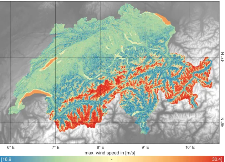
The map of predicted wind speeds for Switzerland is presented in Figure 4. The model was build using the following hyper parameters:
• number of boosting iterations = 4500,
• learning rate = 0.001,
• minimum samples per leaf = 8,
• max. tree depth = 2.
5. RESULTS, CONCLUSION
The feature importance shows that two of the top three features are as expected altitude and TOPEX. The importance of the altitude can be explained with increasing heights leading to a terrain being generally less sheltered by vegetation or topographic phenomena and hence wind can travel freely in higher spheres. This leads to stronger winds striking less sheltered surroundings. The TOPEX score can be seen as a combination of different classic values derived from DEMs (e.g. Slope, Curvature, etc.), it’s also a strong tool for determining sheltered areas in which wind is unable to reach higher speeds. The CLC dataset is also one of the main explaining predictors. Given its high diversity of classification, this feature is a real improvement when it comes to describing the topology and presumably also with regard to the associated roughness. Also, the classes of water areas are a huge benefit in the prediction. The other important class are the areas with little or no vegetation, presumably because of the linkage to the declining density of vegetation with increasing altitude. The importance of the both TRI features shows that the roughness is of major influence on the prediction of wind speeds, on small scales of 30 meters as well as on bigger scales of 1000 meters. The importance of the aspect is explained by the dominant wind directions over Europe, which is the west-wind-zone. This is also the direction of the most severe storms.
Figure 4: Map of predicted maximum wind speeds over Switzerland
train error is still reduced. If overfitting was a problem in this model the test error should start raising again as soon as the model is biased by the train set.
The low r² of 0.58 is an indication for the model being able to describe the relationship between features and measured values at least to some extent, but still the goal value here would be around 0.9 to 0.75. This would show a good correlation not biased by an overfit. The rather low value scored here is another sign for the underfiting problem of the model. Nevertheless the RMSE value, within the cross-validation, of 3.42, is the best value reached within the investigations on the prediction of wind speeds in Switzerland using regression methods. This shows that BRTs are a powerful tool for predicting wind speeds over huge areas with a highly differentiated terrain.
A visual interpretation of the predicted map shows that the particular model used in this work is capable of predicting wind speeds, at least on a bigger scale. This is indicated by the distribution of the predicted wind maxima. It is clearly visible that the highest wind speeds are predicted on mountain tops and larger lakes. This is what you would expect to happen in the real world. The reasons for wind maxima at mountain tops have been described above. Lakes are windy because of the wide open space with the wind not being chocked off by roughness or bigger obstacles. Accordingly the wind at larger lakes is predicted to be stronger than at smaller lakes. Another indicator for the plausibility of the results achieved with the method of this work is that smaller valleys show lower wind speeds as mountain tops or large plains. This result again is as expected for the real world. However all these predictions work only on large scale but fail when it comes to small-scale dynamics of wind flow. For example, the dynamics in two neighbouring valleys can differ completely from each other.
Therefor in future work superior descriptors have to be found in order to describe the wind flow in a more precise manner. Promising examples may be features using flow routing algorithms or computational fluid mechanics algorithms to model wind flow. Making use of multi-spectral images for a more complete land classification of a specific area and the use of a DEM of a higher resolution could also improve the predictions. Using data of bigger scale from overall wind flow dynamics over Europe or Switzerland can provide another options. Also, the general gathering of a bigger, more complete dataset is an option that has to be taken into account.
ACKNOWLEDGEMENTS
The authors would like to thank the Swiss Meteorological Service Meteo Swiss for providing the wind speed measurement data and maintaining the IDAWEB network.
REFERENCES
Büttner, G., 2014. “CORINE Land Cover and Land Cover Change Products.” In: Land Use and Land Cover Mapping in Europe: Practices and Trends. Remote Sensing and Digital Image Processing, edited by I. Manakos and M. Braun, pp. 55-74. Dordrecht: Springer.
Chapman, L., 2000. “Assessing topographic exposure”. Meteorological Applications 7, pp. 335-340.
Burbank, D. and Alsdorf, D., 2007. “The shuttle radar topography mission.” Reviews of Geophysics.
Hastie, T., Tibshirani, R., Friedman, J., 2014. “Boosting and Additive Trees.” In: The Elements of Statistical Learning. Data Mining, Inference, and Prediction, edited by I. Manakos and M. Braun, pp. 55-74. Dordrecht: Springer.
Klawa M. and Ulbrich U., 2003: A model for the estimation of storm losses and the identification of servere winter storms in Germany, Institute of Geophysics and Meteorology, University of Cologne.
Li, Z., Zhu, Q., Gold, C., 2005. Digital Terrain Modeling - principles and methodology. CRC.
Munich RE, Windstorm – Major global natural hazard. URL https://www.munichre.com/touch/naturalhazards/en/naturalhaza rds/meteorological-hazards/storm/index.html (accessed 3.29.16)