Dynamic modeling of a compressed air energy storage system in a grid connected photovoltaic plant

FEDERAL UNIVERSITY OF MINAS GERAIS

PROGRAM OF GRADUATION IN MECHANICAL

ENGINEERING

Dynamic Modeling of a Compressed Air Energy Storage System

in a Grid Connected Photovoltaic Plant

Author: Ahmad Arabkoohsar

Supervisor: Ricardo Nicolau Nassar Koury

Co-Supervisor: Luiz Machado

Dynamic Modeling of a Compressed Air Energy Storage System

in a Grid Connected Photovoltaic Plant

This work is presented to the Program of Graduate Studies in Mechanical Engineering of Federal University of Minas Gerais for obtaining a PhD degree in Mechanical

Engineering.

Concentration Area: Energy and Sustainability

Supervisor: Ricardo Nicolau Nassar Koury Co-Supervisor: Luiz Machado

Federal University of Minas Gerais - UFMG

Belo Horizonte

Program of Graduation in Mechanical Engineering

Av. Antônio Carlos, 6627 - Pampulha - 31.270-901 - Belo Horizonte – MG. Tel.: +55 31 3499-5145 - Fax. +55 31 3443-3783

www.demec.ufmg.br - Email: [email protected]

Dynamic Modeling of a Compressed Air Energy Storage System

in a Grid Connected Photovoltaic Plant

Ahmad Arabkoohsar

The dissertation is defended on April 18, 2016. The examiner bank selected by the board of Program of Graduation in Mecanical Engineering of Federal University of Minas Gerais (UFMG) for this qualification exam which is for defending the research proposal given for obtaining a PhD degree in the area of Energy and Sustainability includes:

PROF. RICARDO NICOLAU NASSAR KOURY

Supervisor–Doctor, Departament of Mechanical Engineering, UFMG.

PROF. LUIZ MACHADO

Co–Supervisor–Doctor, Departament of Mechanical Engineering, UFMG.

PROF. RALNEY NOGUEIRA DE FARIA

Examiner–Doctor, Centro Federal de Educação Tecnológica de Minas Gerais, CEFET -MG.

PROF. RAPHAEL NUNES DE OLIVEIRA

Examiner–Doctor, Centro Federal de Educação Tecnológica de Minas Gerais, CEFET -MG.

PROF. ANTONIO CARLOS LOPES DA COSTA

Acknowledgement

First of all, I thank my compassionate and merciful God for letting me go successfully through all the difficulties and destining this beatiful fate for me to feel such wondeful. Thank you Lord.

I proudly dedicate this PhD thesis to the three angels of my life, i.e. my lovely and patient parents and my devoted wife who endowed themselves so that I could just concentrate on my research career and nothing else. Words cannot express how grateful I am to you all for all of the sacrifices that you have made. Undoubtedly, your prayer was what brought me thus up.

Next, I would like to express my special appreciation and thanks to my supervisor Prof. Ricardo N. N. Koury, my tremendous mentor, for encouraging me thorough my PhD study and for trusting me in one by one of my research project steps. I also thank my kind and helpful advisor, Prof. Luiz Machado, for all his kind supports. He was, surely, the best lecturer that I have ever seen. I do appreciate my former advisor, Prof. Farzaneh -Gord from Shahrood University of Technology of Iran, for his very beneficial adv ices on my dissertation and other our joint research projects over this 2.5 years. He has got a very big heart and has a unique character.

The last but not the least, I’m really thankful to all of my good friends for their valuable

The main problem of renewable energy power plants is the intermittency of the source of energy. Therefore, instantaneous variations of power demand could not be properly recovered. For overcoming this problem, the best solution, by far, seems to be employing energy storage systems and reclaiming the stored energy by the time of demand. Among all possible energy storage systems, compressed air energy storage (CAES) system is the most efficient candidate due to its high efficiency, lower cost of capital and being environmentally friendly. In spite of huge numerical, theoretical and experimental works conducted on CAES technology, dynamic modelling of a CAES system in a renewable energy source power plant with actual fluctuations has never been studied. On the other hand, as Brazil lies among top countries of the world in terms of solar irradiation reception, and pay attention to the fact that not many solar power plants have been installed in the country yet, this thesis presents a dynamic modeling of a CAES system in a large scale grid connected photovoltaic (PV) plant in Brazil. For this power generation system, it is shown that a CAES system with 50 MW capacity for a PV farm with 100 MWp capacity and a power sales strategy of equal to 70% of its monthly-instantaneously averaged energy production can efficiently damp the power ramps of the power plant and minimize the financial fines that power plant can be exposed to due to its sharp ramps. However, it was also concluded that this power generation system can be enhanced in terms of energy and exergy performance if there is an extra source of energy parallel to the power plant output. As a result, the feasibility of utilizing the power output of a power productive natural gas pressure drop station, also known as city gate station (CGS), along with the first power generation system is studied. The results of simulations prove that not only the energy and exergy efficiencies of the power plant increase considerably, but also the CAES system capacity decreases and the power sales strategy of the power plant is modified considerably.

O principal problema de usinas de energia renováveis é a intermitência da fonte de energia. Portanto, as variações instantâneas da demanda de energia não poderia ser devidamente recuperado. Para resolver este problema, a melhor solução parece estar empregando sistemas de armazenamento de energia e recuperar a energia armazenada no momento da demanda. Entre todos os sistemas de armazenamento de energia possíveis, sistema de armazenamento de energia de ar comprimido (CAES) é o candidato mais eficiente, devido à sua alta eficiência, menor custo de capital e ser ambientalmente amigável. Apesar de enormes obras numéricos, teóricos e experimentais realizados em tecnologia CAES, modelagem dinâmica de um sistema CAES em uma usina com fonte de energia renovável com as flutuações reais nunca foi estudada. Por outro lado, o Brasil encontra-se entre os principais países do mundo em termos de recepção de irradiação solar, e prestar atenção ao fato que nao muitas usinas de energia solar nao foram instalados no país, no entanto, esta tese apresenta uma modelagem dinâmica de um sistema CAES em uma grade escala planta fotovoltaica (PV) conetado ao rede no Brasil. Para este sistema de geração de energia, mostra-se que um sistema CAES com capacidade de 50 MW para uma fazenda PV com capacidade de 100 MWp e uma estratégia de vendas de eletricidade igual a 70% da sua produção média instantaneamente-mensal pode eficientemente amortecer as rampas de energia de a usina de energia e minimizar as multas financeiras que usina podem ser expostos a devido à sua rampas acentuadas. No entanto, concluiu-se também que este sistema de geração de energia pode ser melhorada em termos de eficiencia de energia e exergia se tem uma fonte adicional de energia paralelo à produção dele. Como resultado, a possibilidade de utilizar a potência de saída de uma estação de reduzir de pressão de gás natural, também conhecida como a city gate station (CGS), juntamente com o primeiro sistema de geração de energia é estudada. Os resultados das simulações provar que não só as eficiências de energia e exergia da usina aumentar consideravelmente, mas também a capacidade do sistema CAES diminui ea estratégia de venda de energia da usina é modificado consideravelmente.

1. INTRODUCTION ... 20

2. COMPRESSED AIR ENERGY STORAGE SYSTEM. ... 27

2.1 CAES Background. ... 27

2.2 CAES System Configuration. ... 30

2.3 A-CAES System Formulation... 37

2.3.1 Energy Performance Investigation... 39

2.3.2 Exergy Performance Investigation... 51

3. PHOTOVOLTAIC TECHNOLOGY ... 58

3.1 Fundamentals of PV Technology. ... 58

3.2 PV Technology Background. ... 60

3.3 PV System Components. ... 63

3.3.1 PV Array. ... 64

3.3.2 Battery. ... 68

3.3.3 Inverter.. ... 69

3.3.4 Charge Controller ... 70

3.3.5 Power Peak Tracker ... 70

3.4 PV System Energy Analysis. ... 72

3.4.1 Solar Irradiation General Formulation. ... 72

3.4.2 Available Solar Irradiation by Various Tracking Modes... 74

3.4.3 PV Cell Formulation ... 78

3.5 PV System Exergy Analysis. ... 82

3.6 Loss Sources and Uncertainty of a PV System... 83

4. CITY GATE STATION ... 86

4.1 Pressure Reduction in Natural Gas Transmission Pipeline. ... 86

4.2 Conventional Configuration of a CGS ... 86

4.3 The Modified Configuration. ... 88

4.4 4.4 Mathematical Modelling of Modified CGS. ... 90

4.4.1 Energy Analysis. ... 90

5.1 PV Farm Equipped with a CAES System. ... 98

5.1.1 PV Farm. ... 101

5.1.2 CAES System. ... 105

5.2 PV Farm Equipped with a CAES System and Accompanied with a CGS. ... 110

5.2.1 Power Productive CGS. ... 111

5.2.2 PV Farm. ... 114

5.2.2 CAES System. ... 114

6. RESULTS AND DISCUSSIONS ... 115

6.1 The Results of Simulation on the First PV Plant Configuration. ... 126

6.2 The Results of Simulation on the Hybrid Power Plant. ... 142

7. CONCLUSIONS ... 162

8. FUTURE WORKS ... 165

FIGURES LIST

FIGURE 1.1 – The schematic of a conventional CAES system. ... 21

FIGURE 1.2 – The schematic of various types of solar collectors. ... 23

FIGURE 1.3 –The schematic diagram of a concentrating solar power plant. ... 24

FIGURE 1.4 –The schematic diagram of a PV farm. ... 24

FIGURE 2.1 – Iowa wind-CAES power plant. ... 29

FIGURE 2.2 – The first configuration proposed for the CAES ... 30

FIGURE 2.3 – The schematic diagram of a CAES system accompanying with a gas turbine plant. ... 31

FIGURE 2.4 – The schematic diagram of the first design A-CAES system. ... 32

FIGURE 2.5 – The schematic diagram of two-TES A-CAES system. ... 33

FIGURE 2.6 – A-CAES system with multiple stage compressor and turbine ... 34

FIGURE 2.7 – The effect of employing multiple stage compressors on the amount of required work... 35

FIGURE 2.8 – Schematic of the A-CAES system equipped with a solar heating system. ... 36

FIGURE 2.9 – The schematic diagram of a simple flat plate solar collector with cross sectional of a single tube... 43

FIGURE 2.10 – The schematic diagram of a flat plate evacuated solar collector with cross sectional of a single tube... 43

FIGURE 2.11 – The schematic of a three-node storage tank. ... 48

FIGURE 3.1 – The schematic diagram of a PV cell. ... 59

FIGURE 3.2 – The PV power production system components. ... 65

FIGURE 3.3 – Schematic diagram of a PV module consisting of NPM branches each with NSM cells in series... 68

FIGURE 3.6 – single solar cell model. ... 79

FIGURE 3.7 – Representative current-voltage curve for a PV cell. ... 80

FIGURE 3.8 – Energy flow diagram of a PV plant . ... 84

FIGURE 4.1 – The schematic diagram of a line heater employed in a CGS for preheating the natural gas stream . ... 87

FIGURE 4.2 – The conventional configuration of a CGS. ... 87

FIGURE 4.3 – The modified configuration of CGS ... 89

FIGURE 4.4 – The control volume selected for exergy analysis of a CGS. ... 94

FIGURE 5.1 – The schematic of the proposed configuration ... 99

FIGURE 5.2 –Brazil’s normal solar irradiation intensity map in 2014. ... 102

FIGURE 5.3 – Plane rotating around north-south axis parallel to the earth’s axis with continuous adjustment. ... 104

FIGURE 5.4 – Various power selling strategies during the day; a) constant power; b) time dependent power. ... 105

FIGURE 5.5 – The schematic of the proposed system. ... 110

FIGURE 5.6 – The arrangement of facilities in the CGS. ... 112

FIGURE 5.7 – The arrangement of facilities in the improved configuration of assumptive CGS in Natal city. ... 113

FIGURE 6.1 – Maximum and minimum average ambient temperature in Natal in 2012. .... 115

FIGURE 6.2 – Hourly-monthly averaged solar irradiation on a horizontal surface with 1 m2 area in Natal. ... 117

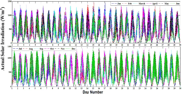
FIGURE 6.3 – Actual solar irradiation on a horizontal surface with 1 m2 area in Natal in 2012. ... 117

FIGURE 6.25 – Total daily energy performance of the CAES unit ... 137

FIGURE 6.26 – Total daily exergy and energy efficiency of the CAES system ... 138

FIGURE 6.27 – Total daily power sold/offset/un-recovered and nightly produced in the power plant ... 139

FIGURE 6.28 – Total daily energy and exergy efficiencies of the power plant ... 140

FIGURE 6.29 – Overall annual statistics of the power production and ramps of the power plant ... 140

FIGURE 6.30 – The results of NPV analysis on the power plant... 141

FIGURE 6.31 – Producible power in the PV farm in presence/absence of the CGS power production in three sample days ... 142

FIGURE 6.32 – Payback period of the power plant with different power sales strategies and CAES sizes ... 143

FIGURE 6.33 – Cavern pressure variation during the three sample days ... 145

FIGURE 6.34 – Expander/Compressor set total work during the three sample days ... 145

FIGURE 6.35 – Expanding/compressing air flow rates during the three sample days ... 146

FIGURE 6.36 – Overall effect of the CAES system on the performance of the PV farm and the CGS power production station during the three sample days ... 147

FIGURE 6.37 – Total daily heating duty of the air heater during the whole year ... 149

FIGURE 6.38 – A single collector solar heating unit performance in the 142nd day of the year ... 149

FIGURE 6.39 – The solar heating unit performance effect on the CAES system in the 142nd day of the year ... 140

FIGURE 6.40 – Fuel consumption reduction in the CAES system by the evacuated tube solar collector system ... 151

FIGURE 6.41 – The inlet natural gas versus ambient temperatures in the CGS ... 152

LIST OF TABLES

TABLE 2.1 – Compressibility formulation constant coefficients values ... 38

TABLE 2.2 – The values of chemical exergy and molar enthalpy of different elements in reference conditions ... 57

TABLE 3.1 – Details of various PV cells available in the market ... 66

TABLE 5.1 – Details of various PV cells and tracker mode utilized in this work ... 103

TABLE 5.2 – Compressors and expanders arrangements in different operational conditions ... 107

TABLE 5.3 – Properties of employed solar collectors ... 108

TABLE 5.4 – The characteristics of the sample PV plant... 109

TABLE 5.5 – The considered CGS technical information ... 112

TABLE 5.6 – The natural gas compositions ... 112

TABLE 5.7 – The characteristics of employed evacuated solar collectors ... 113

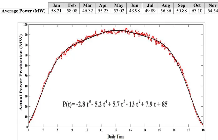
TABLE 6.1 The monthly average actual producible power during the daily hours of each month ... 123

A Heat transfer area (m2)

c Specific thermal capacity (kJ/kg.oC)

cp Specific thermal capacity in constant pressure (kJ/kg.oC)

CAES Compressor air energy storage system CGS City gate station

D and d Diameter (m)

Dh Hydraulic diameter (m)

e Electron charge (J/V)

E Overall energy of control volume (kJ)

E̅ Heat exchanger effectiveness FF Fill factor

F’ Collector efficiency factor FR Collector removal factor

Gsc Solar Constant (W/m2)

h Specific enthalpy (kJ/kg)

h̅ Convective heat transfer coefficient (W/m2.K)

ĥ Molar enthalpy (kJ/kmol)

H Enthalpy (kJ)

I Current (Ohm)

I Solar irradiation on a horizontal surface on the earth (W/m2.hr)

Ib Beam component of solar irradiation (W/m2.hr)

Id Diffuse component of solar irradiation (W/m2.hr)

Io Solar irradiation on a horizontal surface beyond the atmosphere (W/m2.hr)

IT Solar irradiation on a slopped surface (W/m2.hr)

İ Irreversibility (kW)

k Thermal conductivity (W/m.oC)

KT Sky clearness index

LHV Lowering heating value (kJ/kg)

m Mass (kg)

N Number

NRSME Normalized root square mean error

P Pressure (kPa)

PE Extra power available for the CAES system (MW)

PE-G Energy shortage in the system (MW)

Pr Prandtl number PR Performance ratio PV Photovoltaic

𝑄̇ Heat transfer rate (kW)

r Radius (m)

R Heat resistance (m2.K/W)

RSME Root mean square error

Re Reynolds number

s Specific entropy (kJ/kg.K)

ŝ Molar entropy (kJ/kmol.K)

S Entropy (kJ/K)

S Absorbed solar radiation (W/m2)

t Time (s)

T Temperature (ºC or K)

U Overall heat transfer coefficient (W/m2.C)

V Voltage (V)

V Volume m3

V̇ Volume flow rate (m3/s)

w Specific work (kJ/kg)

W Work (kJ)

Ẇ Work rate (kW)

Y Yield

Z Compressibility factor Greek Symbols

φ Latitude angle

Slop Angle and Compression ratio

′ Expansion ratio

ρg Reflection solar irradiation coefficient

Incident angle

z Zenith angle

Surface azimuth angle

s Solar azimuth angle

Efficiency

λ Time step

ξ Overall energy efficiency Exergy efficiency

σ̇ Exergy generation rate Specific exergy

Ѱ Exergy

Γ Uncertainty

Subscriptions

a Air

am Ambient

c Collector

C Compressor

ca Cavern

che Cooling heat exchanger cm Collector module dah Diesel air heater

e External

f Working fluid

ft Fire tube

fu Fuel

g Generator

h Heater

i Internal NG Natural gas

o Dead state

OC Open circuit PM Parallel module rev Reversible SC Short circuit

she Solar heat exchanger SM Series modules SS Solar set

sst Solar storage tank sth Hot storage tank

1.

Introduction

Nowadays, most of the required energy all over the world is provided by fossil fuels. There are two main problems that prohibit using such sources of energy. The first problem is that the fossil fuels are getting more expensive everyday as the underground reservoirs of such fuels are getting discharged and as a result, these sources of ener gy are becoming increasingly rare. The next problem is that burning fossil fuels for providing the required heat has serious negative impacts on the environment. This is why employing renewable and sustainable sources of energy in both industrial and domestic applications has been the concern of corresponding experts over the recent decades (Farzaneh-Gord et al., 2011). One of the main sections that these sources of energy are widely used nowadays is power generation in both standalone and grid connected forms.

However, the main problem of renewable energy power plants is that the source of energy is inherently intermittent like wind and solar energies that are unstable and erratic dramatically. Therefore, instantaneous variations of electricity demand of the consumer, which could be either an individual consumer or a national electricity distribution grid, may not be accurately responded (Botterud, 2014). For overcoming this problem in a renewable energy source power plant, firstly, unpredictable and steep ramps in the electricity demand of the consumer, and secondly, the ramps in the source of energy should be taken into account. Therefore, accurate forecast would eliminate these problems entirely (Diagne et al., 2014).

attention in the recent years (Breeze, 2014). Figure 1.1 shows the schematic diagram of a CAES system. According to the figure, in a CAES system, the extra power for being stored is used to run a compressor that intakes ambient air. The compressed air, which is also hot now, after passing through a heat exchanger, is stored within an air storage reservoir. The compressed air could be reclaimed to pass through a turbine and produce work when required. In order to meet the desired temperature before the expansion process, the air stream is warmed up by an auxiliary diesel air heater.

FIGURE 1.1 – The schematic of a conventional CAES system: C: compressor, T: turbine, G: generator, ASR: air storage reservoir, DAH: diesel air heater

The primary question about a CAES system is about its performance in a renewable energy source power plant under real operational circumstances. In fact, although the CAES technology has been well studied and progressed over the last years, no professional and specific work on dynamic modeling of a CAES system has been addressed in the literature yet. Therefore, the main goal of this dissertation is accomplishing a comprehensive energy and exergy analysis on a CAES system dynamically while operating in a renewable energy source power plant. For the sake of having a more accurate and precise simulation, in the first step of this project, a renewable energy source power plant with real transient operational conditions in Brazil is considered and the CAES performance in this power plant is simulated for a whole year.

by the earth. This amount of energy is almost well above 7500 times the world’s total annual energy demand (Midilli et al., 2007).

Solar energy technologies include solar heating, cooling, photovoltaics and agriculture and this wide range of application caused it to play an important role to solve some of basic energy problems of the world. Solar technologies are generally known as passive and active solar techniques depending on the matter they harness and convey solar energy. Active solar techniques consist of using photovoltaic panels or solar thermal collectors to profit the energy of the sun. Passive solar techniques, on the other hand, are those in which the energy of the sun is utilized without any special instrument to be employed; for example, orienting a building toward the sun to harvest the sun light and heat (Farzaneh-Gord et al., 2014).

a) Flat Plate Collector b) Evacuated Collector c) Concentrator Collector

FIGURE 1.2 – The schematic of various types of solar collectors

Thirugnanasambandam et al. (2010) presented various types of solar thermal technologies such as solar water heaters, solar cookers, solar driers, solar ponds, solar architecture, solar air-conditioning and solar chimneys. Norton (1999) presented the most common applications of industrial process heat presenting the solar industrials and agricultural applications background and samples. Sharma et al. (2009) reviewed solar energy drying systems consisting of passive and active solar dryers. Bal et al. (2009) presented a review of solar dryers with thermal energy storage facilities employed in agricultural industry. Muthusivagami et al. (2010) thoroughly reviewed solar cookers with and without thermal storage equipment. Muneer et al. (2006) have studied the prospects of solar water heating for textile industry in Pakistan. Benz et al. (1998) presented the planning of two solar thermal systems generating process heat for a brewery and a dairy in Germany. In another work, Benz et al. (1999) presented a study for utilizing non-concentrating collectors for food industry in Germany. The aforementioned works are only a few out of thousands of studies accomplished on the solar heating systems and many others could also be referred in the literature.

FIGURE 1.3 – The schematic diagram of a concentrating solar power plant

On the other hand, in direct solar power generation method photovoltaics (PV) cells are used to convert directly sunlight into electricity using the photovoltaic effect. PV technology has been widely used to provide power in both large and small scales. In a PV system, sunlight is directly converted into electricity by striking PV panels (Khadidjaa et al., 2014). In small scale, standalone PV systems (not connected to the grid) are used for producing power where there is no access to electricity distribution grid or even for reducing electricity bills in grid connected places. In large scale, on the other hand, large PV farms can be built to provide the required electricity of cities, big factories and so on (Thanaraka and Sae-Erib, 2012). Figure 1.4 shows the schematic of a PV farm.

According to the introduction given for solar energy and considering this fact that Brazil is among top countries worldwide in terms of solar irradiation, a PV farm has been chosen to host a CAES system for this study. In this regards, in this dissertation, first of all, a comprehensive introductions and backgrounds about the PV and the CAES technologies are presented and detailed formulation and mathematical model related to both of these technologies are given. The proposed configuration is presented and comprehensive exergy and energy analysis formulation related to this system is also given. As the power plant is supposed to be in Brazil, the best location in terms of the most available solar irradiation all over the country is selected.

One problem that all renewable energy source plants have is determining the most economically efficient pattern based on which the power plant sells power to the grid. In fact, the amount of power that each power plant should supply for the grid is defined in advance based on mutual agreement between the grid and the power plant and there will be huge penalties for the plant in case of any power ramp comparing to the agreed value. There are mainly two different types of power sale pattern as daily constant power strategy and time dependent power strategy. Overall, as accurate prediction of the intensity of renewable energy sources is not possible, even in presence of an energy storage system, the power plant could not guarantee how much power can exactly supply to the grid in every moment. Pay attention to the fact that, the more power is sold to the grid, the higher revenue is earned by the plant, one should find a solution by which not only the power plant maximizes the total annual amount of power sold to the grid, but also minimizes the total annual financial fines. Therefore, the most efficient power sales strategy of the PV plant is found in the next step.

After simulating this power plant, a second proposal is given to improve the performance of the first configuration proposed. In fact, this proposal aims at enhancing the stability of the power produced and increasing the revenue of the previous PV plant. This system adds a large scale natural gas pressure drop station, which is called city gate station (CGS) to the previous PV plant configuration. After introducing CGSs and calculating the producible power by such a system, the proposed hybrid configuration is illustrated and detailed mathematical model about it is given. The best power sales strategy along with determining the most optimal CAES size for this hybrid system are chosen and comprehensive exergy and energy simulation on the optimized configuration of the power plant while working under real circumstances for a whole year is accomplished.

As the main goal of this work is simulating and dynamic moddeling of the performance of a CAES system in a PV farm, therefore, the CAES technology should be first introduced. This chapter present a detailed background, information and mathematical moddeling of the CAES technology.

2.1CAES Background

Substantiated by issues of energy security, climate change and rising fossil fuels prices, many countries around the world lead an energy policy focusing on energy efficiency and increasing the share of renewable energy sources (International Energy Agency and Organization for Economic Co-operation and Development, 2015). In some countries and regions, these policies also involve increasing the share of combined heat and power (CHP) (European Commission, 2002 and 2008). Such energy policies lead to the challenge of balancing electricity supply and demand (Andersen and Lund, 2007). Various technological options have been analyzed and several measures have been implemented including changes in the regulation of distributed CHP plants (Eriksen, 2001). The different technological options in question include electric boilers and heat pumps (Blarke and Lund, 2007), flexible demands (Meibom et al., 2007), electricity for transportation (Mathiesen et al., 2008), re-organization of energy conversion in relation to waste treatment (Münster, 2007) and various energy storage options (Mathiesen and Lund, 2009).

The CAES is a modification of the basic gas turbine technology, in which low-cost electricity or extra electricity available is employed to actuate some compressors and produce compressed air and store this compressed air in an underground reservoir. This is could be reclaimed for producing power when required. Thus, the air should be heated and expanded in a gas turbine in order to produce electricity during peak demand hours. As it derives from gas turbine technology, the CAES is readily available and reliable (Kondoh et al., 2000).

The first CAES plant was commissioned in Huntorf, Germany in 1978 to provide peak power for a gas turbine plant. The Huntorf plant, which is still in operation, stores up to 310,000 m3 of compressed air at a pressure range of 44–70 bar in two salt caverns and can produce up to 290 MW of electricity at full capacity for 4h at an air discharge flow rate of 417 kg/s (Raju and Khaitan, 2012). The second utility scale CAES plant was also commissioned in 1991 in McIntosh, capable to generate 110 MW of electricity at full capacity for 26h with an air discharge rate of 154 kg/s. It stores up to 540,000 m3 of compressed air at a pressure range of 45-74 bars in a salt cavern (Powersouth, 2013).

FIGURE 2.1 − Iowa wind-CAES power plant

interact with each other. Salgi and Lund (2008) performed a technical system analysis with an increased wind power penetration in Denmark. The mentioned study, however, does not take into account the economic feasibility of a CAES plant. Swider (2007) presented a stochastic model for analyzing the economic competitiveness of CAES in a system with growing wind power penetration. The study concludes that the CAES can be economically competitive with other technologies in a system characterized by the phasing out of nuclear power. While stressing the importance of flexible technologies, the study does not compare CAES to other such available technologies.

2.2CAES System Configuration

The first configuration proposed as a CAES system was the simplest configuration proposed for this objective ever. This proposal was given by 1940 (Kousksou et al., 2014).

FIGURE 2.2 − The first configuration proposed for the CAES; M: motor, C: compressor, ASR: air storage reservoir, DAH: diesel air heater, T: turbine, G: generator

a turbine shaft which is coupled with an electricity generator rotor. This process causes the generator to produce the required power. Note that the expanding air mass flow rate depends on the amount of power required in every moment.

Although the idea given by this system was a novel and innovative proposal, the net efficiency of such a system was not that much satisfactory that made too expensive the power produced by this system. A variety of newer CAES designs have been proposed in the past few decades to improve the storage efficiency of conventional CAES plants. The Energy Storage and Power Corporation in the 1990s proposed the first modified version of the conventional configuration of CAES system based on pairing CAES plants with conventional gas turbines. The main idea of this approach is eliminating the air heater in the CAES facility and utilizing the exhaust stream from the gas turbine instead of the combustor to heat the compressed air and thus improving the overall efficiency. Figure 2.3 shows the schematic diagram of the CAES system accompanying with a gas turbine plant.

FIGURE 2.3 − The schematic diagram of a CAES system accompanying with a gas turbine plant; C.C: combustion chamber, H.E: heat exchanger

In contrast to this approach which focuses on waste heat recovery during the discharging process, Adiabatic CAES (A-CAES) design is based on storing the heat generated in the air stream through the compression process in a thermal energy storage facility. This stored heat then would be utilized to heat the compressed air during the generation (expansion) process and thus lower (or even eliminate) the fuel consumption of the CAES plant. This concept was introduced in the 1980s and the interest in this concept is recently renewed both in Europe and the United States (Porto et al., 2013). Figure 2.4 illustrates the schematic diagrams of a simple design A-CAES system.

FIGURE 2.4 − The schematic diagram of the first A-CAES system design; TES: thermal energy storage

According to the figure, the thermal energy storage system is added to the first configuration proposed for CAES system. In this way, one could collect the heat generated in the air stream while being compressed. This is usually done by some heat exchanger s in which water or industrial oils act as the working fluid. The heated working fluid is then stored in the TES and at the time of power production, this heat is transferred to the expanding air stream. This procedure also takes place in another heat exchanger. After this heat exchanger, in case the air has not met the desired temperature, the auxiliary air heater provides the extra heat required.

high temperature compressors, and high pressure expanders. For example, in the above system, using only one TES could not be so effective because a high gradient inside the tank is needed to reach two completely different boundary conditions inside the tank: high temperature when it goes to the turbine (top side of the tank) and low temperature when enters the storage tank (bottom side). For solving this problem, as another step of modification on the CAES system configuration, it was proposed to use two separate TESs (cold and hot). Figure 2.5 shows the schematic diagram of an A-CAES system with two separate cold and hot TESs.

FIGURE 2.5 − The schematic diagram of two-TES A-CAES system

Although the system shown in figure 2.5 has a reasonable efficiency comparing to the previous configurations, it was not the most efficient system proposed ever. In the next proposal, employing multistage compressors and expanders by which the adiabatic processes in the compressor and expanders approached isothermal processes was proposed. Therefore, train mode of exchanging heat in both giving and getting heat could increase the efficiency to more values up to almost 80% by reducing the compressor inlet temperature and increasing the turbine outlet temperature. This configuration is illustrated in figure 2.6.

FIGURE 2.6 − A-CAES system with multiple stage compressor and turbine

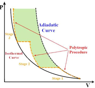
FIGURE 2.7 − The effect of employing multiple stage compressors on the amount of required work

According to the figure, the least amount of required work is for an isothermal process. In a sharp contrast, the maximum amount of work required for the compressor is when the process is adiabatic. Having a compressor which works in an isothermal process is impossible practically. However, one could approach this state by employing multiple stage compressors. In such case, the work of each compressor is adiabatic; however, by using intercoolers one could reduce the next stage compressor significantly and as a result, the work required in the next stage reduces remarkably. The work implemented by the whole compressor unit is called a polytropic process. The green area represents the amount of work reduction caused by employing multiple stage compressors comparing to the amount of work required for a single stage compressor. Note that, by the same approach, the effect of employing multiple turbines on increasing the expansion process efficiency could be explained as well.

FIGURE 2.8 − Schematic of the A-CAES system equipped with a solar heating system; SST: solar storage tank, SCS: solar collector series, SHE: solar heat exchanger

As the figure shows, in expansion process, firstly, the air steam should pass through the solar heat exchangers to be warmed up to possible temperatures. Then, the hot heat exchangers are employed to heat the air stream. In final stage, if still required, the auxiliary heater could also be used. Note that, the solar heat exchanger is supported by hot water produced by solar heating unit including a flat plate collector module and a solar storage tank. In fact, the solar collectors, during the day, collect solar heat and produce hot water. This hot water is then stored in a storage tank and is used in production mode.

savings on fuel (used for heating purposes) can make the D-CAES system cheaper compared to the conventional CAES in certain situations. The intensity and fluctuations of the heat load, size and fluctuations of the electric load, distance between the heat load and storage facility, and the fuel and construction costs are the major players in this tradeoff. This configuration is, however, helpful only when there is a conventional CAES system and another system with heating demand. Therefore, this system is out of this work scope.

2.3A-CAES System Formulation

As it was claimed before, the configuration shown in figure 2.8 is the most efficient system among all CAES systems. Therefore, this configuration is the target CAES system which is used in this work and the mathematical model of this configuration is presented in this section.

Before continuing the discussion, there is an important issue that should be taken into account. The problem is that whether or not the working fluid (air) can be considered as an ideal gas?

In this regard, one should calculate the compressibility factor of air entering and exiting the compressors by calculating the compressibility factor of the air at each stage (Wark and Richards, 1999).

                              2 r 2 r 2 r 3 r 4 5 r 2 r r υ ξ exp υ ξ λ υ T c υ D υ C υ B 1 Z (2.1)

In which, B, C, D, vr and Tr can be given by the following equations.

(2.2)

Where, v, Tc and Pc are specific volume, critical temperature and critical pressure

of the working fluid (specifically air here), respectively. Also, the other parameters in the above equations, which are all constant, can be found in the following table (Wark and Richards, 1999). c c r c r r 2 1 3 r 3 r 2 1 4 2 r 3 r 2 1 P RT υ υ ; T T T ; T d d D ; T c T c c C ; T3 b T b T b b

TABLE 2.1 − Compressibility formulation constant coefficients values

Constant Value Constant Value

b1 0.1181193 c3

0

b2 0.265728 c4

0.042724

b3 0.154790 d1

0.0000155488

b4 0.030323 d2

0.0000623689

c1 0.0236744 λ

0.65392

c2 0.0186984

0.060167

Employing the above formulation, if the value of compressibility factor is obtained equal to 1, the gas can be considered as an ideal gas; otherwise, it should be considered as a real gas and appropriate formulation should be adopted.

Note that in mathematical modelling of the system, overall, the following assumptions are taken:

a. The effect of ambient air humidity on the CAES system performance is neglected as the CAES systems always take advantage of dehumidifiers.

b. The air throughout the compression and expansion process in the CAES system is considered as ideal gas. Considering the maximum pressure and the temperature of air in the system, this assumption is totally reasonable.

c. The compressors, expanders and heat exchangers in the CAES system could react to the instantaneous fluctuation of depending parameters very fast and the variations of kinetic and potential energies through them are assumed to be negligible.

d. The processes of compressors and expanders are considered as isentropic procedures.

e. The heat exchangers and storage tanks in the CAES system are assumed to be totally insulated.

isolated, has usually enough time to approach the ambient temperature when the expansion unit is in standby state.

In the target configuration, for the sake of simulating the system, five separate control volumes could be defined including the compression unit, the air storage reservoir (cavern), the solar heating unit, the expansion unit and the auxiliary air heater.

2.3.1 Energy Performance Investigation

The general format of the first law of thermodynamics or energy conservation law for a control volume is (Wark and Richards, 1999):

(2.3)

Where, Q̇ and Ẇ refer to the amount of heat and work exchanged between the control volume and the environment respectively. ṁ, h, Ve and z also represent the mass flow rate, enthalpy, velocity and potential term of the flows incoming or outgoing into/from the control volume. EC.V also refers to the total energy of the control volume including internal

energy (U), kinetic energy (KE) and potential energy (PE). Note that the above equation subscripts i and e represent the inlet and outlet conditions respectively. In addition, the mass conservation law for the control volume (if applicable) can be written as:





e i 1 λ m t Δ m m

m  





Where, m is the total mass of the control volume and the superscript λ counts the

operational time steps of the control volume.

The first law efficiency, based on the definition, shows what portion of the inlet energy in the system has been effectively employed to produce power output by the control volume. Thus: input Energy output energy Useful 



After presenting the fundamentals of the first law of thermodynamics, one could analyze all the system components individually. In the first control volume i.e. the







 2e _e

e e i 2 i i i C.V C.V C.V _gz 2 Ve h m gz 2 Ve h m W Q dt

compression unit, based on the conception, the compressor set total work (Ẇ_C) is equal to the extra produced electricity (PE) multiplied by the compressor set overall efficiency ( C).

C E C

P

W





Due to the high mass flow rate and pressure required in the CAES system, centrifugal compressors are selected to be used in this work for which isentropic efficiency is considered to be equal 85% (Li, 2013).

Knowing the compressor efficiency and employing simple thermodynamic correlations, one could easily calculate the specific isentropic work (wC,is) and subsequently

actual work (wC,act) of compressors and, subsequently, the compressor actual outlet

temperature (TC-e):

e p

i -C i p act , C e -C

c

T

c

w

T

 





Where, TC-i is compressor inlet air temperature and cp-i andcp-e are air specific heat

capacity at compressor entrance and exit respectively. As cp value depends on the

temperature, therefore, iterative solution is required here.

Calculating the specific works of all compressors, one can obtain the total air mass flow rate (ṁC,t) intake into the compressor set as:





 _{C,t c c}

t C, t

C,W W m w

m   (2.8)

The first compressor inlet air temperature is known (ambient temperature) and energy analysis on the cold heat exchanger series could reveal the value of inlet air temperature for the other compressors.

The rate of heat transferred from the air to the working fluid (which will be industrial oil) in each heat exchanger (cooling heat exchanger series) is given by:

lm che che

che U A T

q   (2.9)

In this equation, Ache is the heat transfer area. Ucheand ΔTlm are respectively the

calculated as:                      i o a lm o f che A A h 1 A A k Δr h 1 U 1 (2.10) (2.11)

Where, Ao, Ai are respectively the internal and external areas of the tube, Alm the

log mean of these values and Δr is difference between the internal and external radiuses of

tube. Also, h̅_a, h̅, and k are convective heat transfer coefficients for the air and working fluid streams and the conductivity coefficient of the tube, respectively. Ti-a, Ti-f, Te-a and Te-f are

respectively the temperature of air and working fluid entering the heat exchangers and the temperature of air and working fluid outgoing from the heat exchangers.

One should note that the flow regime for the working fluid is laminar due to the high viscosity of the industrial oil while for the air clearly a turbulent regime is expected. Thus, for calculating the value of convective heat transfer coefficients, the following equations are used (Incropera and DeWitt, 2002).

i a 0.4 a 0.8 a a

D

k

Pr

Re

0.023

h



h f f

D

k

4.36

h



In which, Rea, Pra, ka, kf, Di and Dh are Reynolds and Prandtl numbers for the air

stream, the thermal conductivity of air and working fluid, the internal diameter for the inner tube and hydraulic diameter for the outer tube, respectively.

Employing the above formulation, the air temperature outgoing from each heat exchanger (Te-a) and the outlet working fluid temperature (Te-f) are calculated by:





i a

e

T

1

E

E

T

T











T_       _



 (2.15)

Where, E̅ is the heat exchanger effectiveness given by:

a p a min min min

che ; C m c

C UA 1

C UA

E  _



  (2.16)

In the above formulation, compressor inlet temperatures are required for calculating the specific work of each compressor. On the other hand, for calculating the compressors inlet temperatures the value of heat exchanger effectiveness is needed. As a result, this formulation will only be calculable with iterative solution.

Finally, by implementing the mass conservation law and the first law of thermodynamics for the hot storage tank (TES 1), one has:



m

m



Δt

m

m

























Where, cf, mhst and Thst are the specific heat, mass and temperature of working

fluid in the cold storage tank respectively. The superscriptions λ and λ+1 also count the

system operational time steps.

For the second control volume (the cavern), from the mass conservation law, one has:



m

m



Δt

m

m















In which, mca is the mass of air encapsulated in the cavern. Also, considering air

as an ideal gas (if possible), the cavern pressure (Pca) could be obtained as:

ca ca ca ca

V

T

R

m

In this equation, Tca is the cavern temperature and is always considered to be

equal to the ambient temperature.

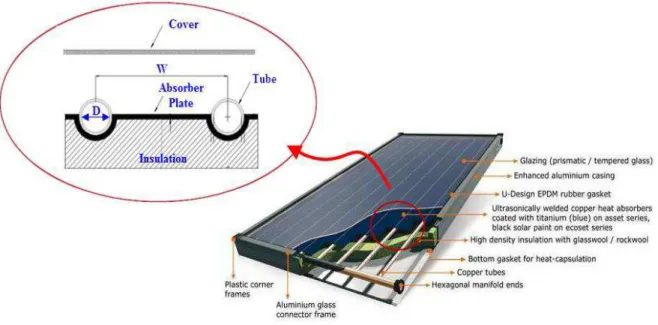
FIGURE 2.9 − The schematic diagram of a simple flat plate solar collector with cross sectional of a single tube

The third control volume is the solar heating system which is hired to provide a portion of the required heat for preheating the air stream before the expansion process. Note that in both cases of employing either flat plate evacuated tube or simple flat plate collectors; similar formulation with minor differences applies for the collectors. Figure 2.9 and figure 2.10 illustrates the schematic diagram of these two collectors with the required dimensions for modelling them.

The obtainable energy by the working fluid through such solar collectors (Q̇ ) could be computed as follow (Duffie and Beckman, 1980):





F A

Qu  c R  l fi  am

(2.21)

Where, Ac, S, Ul, Tfi and Tam are respectively the collector absorber surface area,

the absorbed solar flux, the overall loss coefficient of collector, the inlet working fluid temperature and ambient temperature. FR is also the removal factor of collector which is given

by:                f f l c l c f f R c m F U A exp 1 U A c m F   _(2.22)

In which ṁf and cf are the working fluid mass flow rate and specific heat

respectively. Also, F′ is the efficiency factor of collector and could be calculated by:





Where, W, a, Dot, Dit, kp and hfi are the gap between the tubes of collector, the

absorber plate thickness, the inner and outer diameters of collector tubes, the thermal conductivity factor of absorber plate and the convective heat transfer coefficient of working fluid through the collector tubes, respectively.

Also, Ul in equation 2.21 is the overall loss coefficient of collector which is the

origin of difference between the two collector types. For a simple flat plate collector it is the summation of three loss coefficients Ut, Ub and Ue which are respectively the loss coefficients

from top, from back and from edge of the collector (Duffie and Beckman, 1980).

e b t

l

U

U

U

U















Where, p, g, Tpm, To and N are the plate and the cover emittance, the absorber

plate average and ambient temperature and the number of glass layers. The other parameters could be calculated by the following equations:



1

0.089

h

0.1166

h





1

0.07866

N



f













0.000051

1

520

C





(2.27)





















T

100

1

0.43

e

In which, h̅wind is wind convective heat transfer coefficient from the upside of the

collector which could be calculated by:

m wind

9.4

Ve

h



The losses coefficient through the back of the collector could be obtained as:

d

A

k

U



Where, k is thermal conduction factor, A is the collector back area, and d is the collector insulator thickness. For the loss coefficient through the edge of the collector also, one has:





_

_

In which, Ac, P, dc, de and ke are the absorber plate area, the collector perimeter,

the collector thickness and the edges insulator thickness and the thermal conductivity factor from the edges. The value of Tpm could also be given by:





l R

c u fi

pm

1

F

U

F

A

Q

T

T









(2.32)

On the other hand, the overall loss coefficient for a flat plate evacuated tube collector is similar to that for normal flat plate collectors by ignoring the conduction and convection heat transfer from the absorber plate to the glass tube since high vacuum normally exists inside the glass tube. Therefore, the overall heat loss coefficient from the collector is calculated by: a g r, a g cv, g p r, l R 1 R 1 1 R U 1       _(2.33)

According to the equation, the overall heat resistance from the collector includes radiative resistance from the absorber plate to the glass tube (Rr,p-g), radiative resistance from

the glass tube to the environment (Rr,g-a) and convective resistance from the glass to the

environment (Rcv,g-a).

Calculating the overall heat transfer coefficient of collector and the other unknown parameters in the above formulation, the obtainable heat from each collector is computed and subsequently, multiplying the number of collector modules by this value, one could calculate the total heat supplied to the system by the solar heating unit. Having the amount of absorbable solar energy by the collector set and obtainable energy by the working fluid, by implementing the first law of thermodynamic on the solar storage tank, one has:

l u sst

f

sst

n

Q

Q

dt

dT

c

m









Where, n, msst and Tsst are the the number of collecto modules, the mass and





f hf

l

m

c

T

T

Q









Where, ṁhf and Tfe are the mass flow rate of hot working fluid injected into the

solar heat exchanger and the temperature of working fluid outgoing from this heat exchanger, respectively. Finally, the temperature of working fluid in the solar storage tank over time could be given by:





T

c

m

Q

Q

T

f sst λ l u 1 λ sst













Note that the last three equations consider the storage tank as a lumped control volume. However, as warmer layers of working fluid lie in upper levels of the storage tank and vice versa; therefore, in order to have an accurate simulation, the storage tank could also be considered as a multi-node tank instead of being simply assumed as a lumped control volume. The number of nodes in a solar storage tank is recommended to be opted equal to 3 (Farzaneh-Gord et al., 2013). Figure 2.11 illustrates the schematic of a three-node storage tank for which the energy balance on each node should be written as:

















Where, Tco, ṁc, TL, To, and ṁL are the temperature and mass flow rate of water

FIGURE 2.11 − The schematic of a three-node storage tank

Also, the function c i

F in this equation specifies which node receives the hot water incoming from the collector modules side.

                Otherw ise 0 1 N i if or 0 i if 0 T T T if 1 T T and 1 i if 1

F s,i 1 co s,i

i s, co c

i (2.38)

In which, Ts,i is the temperature of node i. Also, the functionFiL determines which node receives the water coming back from the solar heat exchanger.

                Otherw ise 0 1 N i if or 0 i if 0 T T T if 1 T T and 1 i if 1

F s,i 1 L,r s,i

i s, r L, L i (2.39)



























0

m

F

m

F

m

m

0

m











Finally, Q̇ in energy balance equation on the storage tank is the rate of energy flow from the storage tank into the heat exchanger can be calculated by:





L i

st F m T T

Q    (2.41)

Note that for the solar heat exchangers the same formulation as hot heat exchangers could be used.

The fourth control volume is the expansion unit. Naturally, the electricity shortage in the PV farm could be offset by the turbo-generator set. Thus, the expander set total work (Ẇ ) could be given by:

G T G E T

P

W





Where, PE-G and T-G are the amount of auxiliary electricity required and the

turbo-generator set overall efficiency, respectively. Taking the value of isentropic efficiency

of expanders ( T,is) into account, the isentropic outlet temperature and isentropic work of each

turbine could be calculated. The actual work of each expander (wT,act) and actual outlet

temperature (TT-e), then, could be given by:

e p i T i p act , T e T is , T is , T act , T

c

T

c

w

T

;

w

w







Just the same as the first control volume, iterative solution is required for calculating the accurate value of TT-e. The total air mass flow rate through the turbine set

(ṁT,t) can be given by:







t T, t

T,

W

W

m

w

Note that the heating heat exchanger series and the solar heat exchanger set are also related to this control volume for which the same formulation as the first control volume could be employed. Also, the formulation presented for the hot storage tank could be used for the cold storage tank. In this stage also, iterative solution is required to obtain the values of different parameters such as the turbine set total mass flow rate, turbines inlet and outlet temperatures, the work done by each expander, the temperature of water outgoing from each stage of solar heat exchanger as well as the temperature of working fluid outgoing from the hot heat exchangers.

For the auxiliary diesel air heater, as the fifth control volume in the target configuration, the amount of fuel (V̇ ) required for providing the required extra heat at each stage of expansion (Q̇ _a ) could be given by:

h dah fu

LHV Q V



 _ (2.45)

Where, LHV and h are respectively lower heating value of the fuel and the

heater thermal efficiency (Arabkoohsar et al., 2014). It should be noted that the air heater is supposed to burn natural gas as its main fuel for which the LHV is 37.8 MJ/Sm3 (mega joule per standard cubic meter) with an efficiency of 50%. Note that Q̇ _a in each stage could also be calculated by:





i -dah e

-dah j

a -p j a j

dah

m

c

T

T

Q









In which, Tdah-e and Tdah-i are the required temperature before expansion and the

auxiliary air heater inlet air temperature, respectively. The superscription j also refers to the number of stage.

It should be mentioned that during compression process, the equations related to the first and second control volume should be solved simultaneously while during the expansion process, the formulas associated with the second, the third, the fourth and the fifth control volumes must be solved at the same time.







In which, SPS is the total daily power produced by the CAES system, IT,cm is the

total solar energy harvested by the collector modules, PE is the extra power used by the

compression unit to compress air and Pfu is total daily energy entered the system by

consuming fuel (calculable by multiplication of the fuel mass flow rate by the fuel LHV). The variable t also refers to hourly time steps from 6 am to 12 pm.

2.3.2 Exergy Performance Investigation

In this section, the formulation related to the exergy analysis of the system is presented. Based on the second law of thermodynamic, the entropy balance for a control volume could be written as (Kargaran et al., 2013):

0

T

T

Q

T

s

m

T

s

m

T

dt

dS

T

m 1 j _j j o e e o i i o C.V

o



























Where, S, ṁ, Q̇ and σ̇_C.V are the entropy, the mass flow rate, the rate of heat transfer and entropy generation in the control volume, respectively.

The exergy of a fluid stream (Ψ) is defined as the maximum work output that can

be obtained from the stream as the fluid state changes reversibly from the given state to dead state. The dead state is a state of system when it is in thermodynamic equilibrium with its environment. Normally, the dead state is taken to be our environment and for many cases it is taken as 298 K and 101.325 kPa where the velocity and elevation relative to the environment

are zero. Indicating the dead state with the subscript o, Ψ is defined as:









_

























gz

2

Ve

s

s

T

h

h

m

m

Ψ





act u rev, C.V W W

I  

 _{  (2.50)}

As it was explained before, the first law efficiency shows what portion of the inlet energy in the system has been effectively employed to produce power by the control volume. Clearly, in many cases this definition, by itself, cannot be a strong criterion to judge the system performance. In such cases, the second law efficiency can be helpful to evaluate the system performance more accurately. In fact, the first law efficiency shows how well energy

is used comparing with an ideal process and the second law efficiency ( ) indicates how well

availability is used [26].

input ty availabili losses and n distructio ty availabili 1 input ty availabili output ty availabili

useful _{ }

 _(2.51)

After presenting this fundamentals on exergy analysis, one could assess the exergy performance of a CAES system. For the compressor set, considering the assumptions taken for the compressors, the entropy balance on each compressor could be written as:





a

C



m



s



s



Where, σ̇_C is the rate of entropy generation through the compressor. In addition, the amount of irreversibility in the compressor is also given by:









o

C

T

m

s

s

I









Finally, defining the second law efficiency for a compressor as the ratio of exergy increase in the fluid through the compressor to the actual work of compressor, the compressor second law efficiency could be calculated as:









C i e o C

h

h

s

s

T

1









For the heat exchangers, on the other hand, regarding the assumptions taken, from the second law of thermodynamic, one has:









che



m



s



s



m



s



s