Contribuição para teoria de placas: análises estruturais de compósitos laminados...

(1)

MAURICIO FRANCISCO CALIRI JUNIOR

Contribuição para teoria de placas: análises estruturais de compósitos

laminados e estruturas sanduíches via formulações unificadas

(2)

(3)

MAURICIO FRANCISCO CALIRI JUNIOR

Contribuição para teoria de placas: análises estruturais de compósitos

laminados e estruturas sanduíches via formulações unificadas

Tese apresentada à Escola de Engenharia de São Carlos da Universidade de São Paulo para obtenção do Título de Doutor em Engenharia Mecânica.

Área de concentração: Aeronaves.

Orientador: Prof. Assoc. Volnei Tita

São Carlos 2015

(4)

AUTORIZO A REPRODUÇÃO TOTAL OU PARCIAL DESTE TRABALHO, POR QUALQUER MEIO CONVENCIONAL OU ELETRÔNICO, PARA FINS DE ESTUDO E PESQUISA, DESDE QUE CITADA A FONTE.

(5)

(6)

(7)

To my parents Mauricio and Maria

(8)

(9)

Acknowledgements

I would like to thank all those who supported me from 2010 to 2015 in the conclusion of this Doctor Thesis. In special:

To the Conselho Nacional de Desenvolvimento e Tecnológico (CNPq) for the financial support (149908/2010-5).

To my friend and tutor, the Associated Professor Volnei Tita, for his guidance and knowledge which made possible the execution and conclusion of this work.

To my parents, whom always encouraged me to pursue the highest goals.

To the Associated Professor Reginaldo Teixeira Coelho for the use of the license of the commercial software Abaqus.

(10)

(11)

“Only those who attempt the absurd will achieve the impossible”

M. C. Escher

“The (atomic) bomb will never go off. I speak as an expert in explosives.”

(12)

(13)

Resumo

CALIRI JUNIOR, MAURICIO FRANCISCO. Contribuição para teoria de placas: análises estruturais de compósitos laminados e estruturas sanduíches via formulações unificadas. 2015. 246 f. Tese (Doutorado) – Escola de Engenharia de São Carlos, Universidade de São Paulo, São Paulo, 2015.

(14)

concordância. Para uma estrutura sanduíche com núcleo macio, o resultado de deslocamento previsto para um carregamento estático chega a 99.8% de concordância e o resultado de uma análise modal da mesma estrutura mostra uma concordância de 99.5% com os resultados de um modelo feito com elementos 3D em um programa comercial de elementos finitos.

(15)

Abstract

CALIRI JUNIOR, MAURICIO FRANCISCO. Contribution to theory of plates: structural analyses of laminated composites and sandwich structures via unified formulations. 2015. 242 p. Thesis (PhD) – School of Engineering of São Carlos, University of São Paulo, São Paulo, 2015.

(16)

shows an accuracy of 99.5%, comparing to the results from a 3D finite element model built with a commercial software.

(17)

Figures

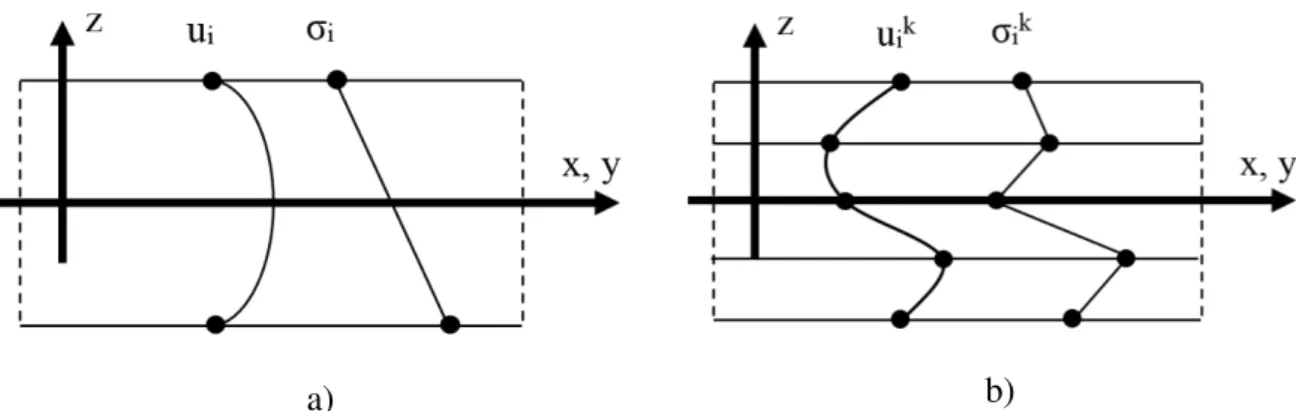
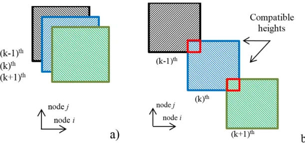
Figure 1. Undeformed and deformed configurations of a material body at time “t” ________ 7 Figure 2. Traction and couple stress vectors on a deformable body ___________________ 10 Figure 3. Equilibrium of traction stresses at a material point _________________________ 12 Figure 4. Momentum balance of a differential volume element ______________________ 13 Figure 5. In-plane local material directions 1-2 and the global x-y orientation for a reinforced ply ______________________________________________________________________ 19 Figure 6. Uniaxial constitutive relations_________________________________________ 20 Figure 7. Generic 3D structure which can be approximated to a 2D structure (L, b >> H) __ 23 Figure 8. a) Polyurethane foam-filled paper honeycomb core. b) foam-filled paper honeycomb core – adapted from Li (2006) ________________________________________________ 32 Figure 9. Isotropic plate representation _________________________________________ 33 Figure 10. Equilibrated forces and moments on a plate element ______________________ 34 Figure 11. Shear functions behavior along the thickness coordinate (z) ________________ 38 Figure 12. Displacement and stress fields in a) monocoque plates and b) multilayred plates 43 Figure 13. Top and bottom faces of consecutive plies ______________________________ 43 Figure 14. Linear and quadratic displacement field for ESL and LW descriptions ________ 46 Figure 15. Components of sandwich structures ___________________________________ 50 Figure 16. CUF acronyms ___________________________________________________ 54 Figure 17. ESL (a) and LW (b) thickness assemblages of the stress, strain and/or displacement variables into the global matrix Kij ____________________________________________ 55

Figure 1κ. Assemblage of matrices (a) K -u and (b) Ku- for ESδ with RεVT into the global matrix Kij ________________________________________________________________ 56 Figure 19. Indexing of the transverse function in GUF _____________________________ 58 Figure 20. GUF acronyms ___________________________________________________ 59 Figure 21. GFEM/XFEM approximation with hat functions _________________________ 80 Figure 22. Elementary sub-domain ____________________________________________ 81 Figure 23. Discretized generic surface: a) square elements; b) triangular elements _______ 87

(18)

(19)

(20)

Figure 76. Case IV: Mesh, load and boundary conditions __________________________ 196 Figure 77. Case V: Mesh, load and boundary conditions __________________________ 196 Figure 78. Through-the-thickness Sx stress via CGF (x = y = l/2) ___________________ 198 Figure 79. Through-the-thickness Sx stress via CGF (x = y = l/2) ___________________ 198 Figure 80. Through-the-thickness Sxy stress via CGF (x = y = 0) ___________________ 199 Figure 81. Through-the-thickness Sxy stress via CGF (x = y = 0) ___________________ 199 Figure 82. Through-the-thickness Sy stress via CGF (x = y = l/2) ___________________ 200 Figure 83. Through-the-thickness Sy stress via CGF (x = y = l/2) ___________________ 200 Figure 84. Through-the-thickness Sz stress via CGF (x = y = l/2) ___________________ 201 Figure 85. Through-the-thickness Sz stress via CGF (x = y = l/2) ___________________ 201 Figure 86. Through-the-thickness Szx stress via CGF (x = 0, y = l/2) ________________ 202 Figure 87. Through-the-thickness Szx stress via CGF (x = 0, y = l/2) ________________ 202 Figure 88. Through-the-thickness Syz stress via CGF (x = l/2, y = 0) ________________ 203 Figure 89. Through-the-thickness Syz stress via CGF (x = l/2, y = 0) ________________ 203 Figure 90. Through-the-thickness dimensionless deflection via CGF (x = y = l/2) ______ 204 Figure 91. Through-the-thickness dimensionless deflection via CGF (x = y = l/2) ______ 204 Figure 92. First two bending modes of vibration via Abaqus 2D, 3D and CGF/LD333 ___ 205 Figure 93. 5th_{and 10}th_{sandwich modes - LD333 ________________________________ 206}

(21)

(22)

(23)

Tables

(24)

(25)

Acronyms

0D Zero-Dimensional 1D One-Dimensional 2D Two-Dimensional 3D Three-Dimensional 6D Six-Dimensional

AWRD Ambartsumian–Whitney–Rath-Das theory CAE Computer Aided Engineering

CFD Computational Fluid Dynamics CLT Classical Lamination Theory CS Coordinate System

DLM Discrete Layer Model DOF Degree of Freedom

DPSE Degenerated/continuum Plate/Shell Element ESL(M) Equivalent Single Layer (Models)

FCSR Face to Core Stiffness Ratio FE Finite Element

FEM Finite Element Method

FESA Finite Element Structural Analyses FSDT First Shear Deformation Theory FSI Fluid Structure Interaction GCS Global Coordinate System

GFEM Generalized Finite Element Method GPVW Generalized Principle of Virtual Work GQ Gauss Quadrature

HSDT Higher Order Shear Deformation Theory HSAPT High order SAndwich Plate Theory IC Inter-laminar Continuity

IP Integration Points

(26)

LFAT Love First Approximation Theory LSAT Love Second Approximation Theory LW(M) Layer-Wise (Models)

MAC Modal Assurance Criterion MQ Multiquadric

MITC Mixed Interpolation of Tensorial Components MWR Method of Weighted Residuals

MZZF εurakami’s Zig-Zag Function PE Plate Element

PVD Principle of Virtual Displacements PVW Principle of Virtual Work

RBF Radial Base Functions

RESL Refined Equivalent Single Layer RMC Reissner–Murakami-Carrera theory. RMVT Reissner’s εixed Variational Theorem SCF Shear Correction Factor

SCT Static Condensation Technique TE Theory of Elasticity

(27)

Chapter 1 - Introduction

1.1 Scope

To perform an accurate structural simulation, there are innumerous variables which need to be handled. Depending on the loading, geometry or constitutive complexity of the problem, very particular approaches might be required. Sandwich structure plates, which are the scope of this work, present an outstanding complexity regarding its microscopic and macroscopic behavior (GIBSON; ASHBY, 1985). These complex laminated structures were devised in order to fulfill different application criteria such as thermal/sound insulation or damping purposes. In addition, such structures are usually applied to reduce weight or increase the energy absorption capacity of a structure.

Intelligent structures may be considered as a class of sandwich structures. These materials most commonly comprise a patch or a layer of piezoelectric material. Such structures are usually applied as monitors or actuators, depending whether the structure was scaled to read (passive) or cause deformation (active) in the structure. The use of intelligent structures in the aeronautical field is very appealing in both active and passive ways. From structural health monitoring to flight control, the applications are countless. Nevertheless, the success of these structures depends on accurate modeling of both mechanical and electrical responses of these, intelligent sandwiches (PIEFORT, 2001, MARINKOVIC; KOPPE; GABBERT, 2006, MORENO; TITA; MARQUES, 2010).

The commercial use of intelligent structures is narrowed due to its complexity and naturally the costs associated, but the use of “regular” sandwich structures is already common

in the field. Some aircraft structures and hulls of boats use sandwich structures to reduce weight and therefore increase the payload. However, the application of these materials on primary structures is rare. Mainly because it is hard to model its tri-dimensional behavior with bi-dimensional assumptions.

(30)

2 Chapter 1 - Introduction

wind blades has drawn much attention because they harvest clean energy (NATIONAL RENEWABLE ENERGY LABORATORY, 2006).

A regular blade diameter of wind turbine generators is 50 m long and they harvest approximately 1.5 MW for wind speeds higher than 12 m/s. However, nowadays, one can find wind turbine blades whose diameters is 120 m long, which can generate around 5 MW. Moreover, there are projects for wind turbines with blades with 200 m long in diameters (NATIONAL RENEWABLE ENERGY LABORATORY, 2006). This is the option to the lack/depletion of good locations for wind farms. In most countries the best or the only locations are already taken, and the solution found is to increase the farms performance by increasing the size wind turbine blades. This is a formidable structural and aeroelastic problem. The use of sandwich structures helps to reduce the weight of this structure but, naturally, it complicates the designing of such structures (IVANELL, 2005, HANSEN et al., 2006).

The aeroelastic problem may be regarded as a type of Fluid Structure Interaction (FSI). The aeroelasticity studies the interaction between body fields, aerodynamic forces and the

structural reaction of the structure (BISPLINGHOFF; ASHLEY; HALFMAN, 1996).

In many aeronautical projects, the deformation related to the deflections of the structure cannot be neglected and the typical rigid body approach may not be sufficient. Aircraft fuselages, wings and wind turbine blades possess large spans which results in strong aeroelastic effects (BISPLINGHOFF; ASHLEY; HALFMAN, 1996).

Recognizing the fact that the aeroelastic solution can get very complex for sandwich structures depending on the loading case, this thesis is devoted to the structural solution only. The fluid solution, which is the loading part of the interaction, needs to be studied separately because the dynamics and magnitude of the fluid solution may range from cruise flight loads to maneuvers loads. This is left as a topic for future works because it involves specific solution methods, including Computational Fluid Dynamics (FERZIGER; PERIC, 2002, VOS et al., 2002). The coupling of both structural and fluid solution is also a field for much research (BHARDWAJ, 1997, ZWAAN; PRANANTA, 2002).

(31)

1.2 Objectives

The main objective of the present work consists on the implementation of a new solution method for laminated composites and sandwich structures based on a Generalized Unified Formulation (GUF) via FEM. A quadrilateral 4-node element will be developed and evaluated using in-house Finite Element program. The C-1 continuity requirements will be fulfilled for the transversal displacement field variable.

In order to comply with the reasons and motivations of this work, this thesis set the following specific goals:

 To review and quote as many as possible the derived plate formulations up to date.  To review and quote as many as possible the solutions methods for plate problems.  To derive a new structural solution method for sandwich structures via FE.

 To derive a FE with partial C-1 continuity.

 To implement the formulated element into an in-house FE code.  To evaluate the accuracy of the code and the element.

 To evaluate the formulation for different plate structures.

 To evaluate the proposed solution method using sandwich structures.

 To conclude about the limitations and potentialities of the proposed solution method.

1.3 Organization

Apart from this chapter, this thesis comprises six other chapters.

Chapter 2 was written to provide a review on the principles of structural mechanics. Since many different structural concepts will be handled in this work, the need for this chapter is clear. Different strain and stress tensors are reviewed and quoted throughout this thesis and a review on the types of these tensor is given. Also, the main constitutive behaviors are briefly quoted as well, mainly because sandwich structures with soft cores demand attention regarding both micro and macroscopic material response.

(32)

4 Chapter 1 - Introduction

becomes 2D. Different ways to derive these 2D plate formulations are presented. Then, the formulations are explained and reviewed according to the thickness of the plate. The thicker the plate is, the more complex (or non-linear) the formulation gets. But besides the thickness factor, the complexity of the theory also increases when the plate is a laminated composite structural material. Sandwich structures fall into this category. Laminated plate theories usually required an integration process in the thickness direction prior to solving the 2D equilibrium equations. Also, the material continuity between plies presents further complications. Finally, the recent Unified Formations for plates and shells are reviewed and their potentially explained.

Chapter 4 elucidates how the accuracy of the laminated plate solution may change according to the solution method. Differential equations are reviewed and the main solution method used in structural analysis are quoted. Global and local solution methods are discussed. However, focus is given to the Finite Element Method (FEM) because it is one of the most common commercial solution methods due to its flexibility in solving different engineering problems. In this chapter it is shown how the elementary equations are derived and whether the governing equations are solved with mixed variables or not for usual plate formulations. Next, the solution of unified plate theories via FEM is discussed for the references quoted. At the end of the chapter, few numerical techniques are explained to clarify the possible errors and issues one may face when solving static or dynamic structural solutions. It is an important chapter to show how Finite Element (FE) formulations may get cumbersome.

Chapter 5 is devoted to the contribution of this thesis. It presents a new solution method for the laminated plate problem. Through FE implementation of a plate element, a generalized unified plate formulation is solved in a more physically consistent way. A four node plate element is derived. An in-house code is developed to test the element. A brief explanation of the code is provided along with explanation on how the thickness integration is carried out.

(33)

of the increase in processing time from one theory to another is given. The results show that the proposed formulation converges to the 3D solutions, and for some cases, outperforms the closed form solutions of the GUF.

Chapter 7 shows the conclusions of this thesis. The main findings are summarized in the

(34)

(35)

Chapter 2 - Principles of Structural

Mechanics

2.1 Strains

In structural mechanics, most of the constitutive laws are derived for the current state of deformation of a material body. However, it is cumbersome to derive the equations of motion for the current state of deformation. Therefore, these equations are normally written in the

δagrangian (or material) configuration, which describes the material body’s position and its

deformation in terms of its initial position. When deriving the equations of the body in terms of its current position, the approach is known as Eulerian (or spatial). Eulerian formulations are more common in fluid mechanics (CHEN; HAN, 1988, CRISFIELD, 1991, ZIENKIEWICZ; TAYLOR, 2000a, 2000b, MENDONÇA, 2005).

Before linking the states of deformation to the corresponding stresses and constitutive laws, the displacement vector and the deformation gradient are derived for a generic material element (Figure 1).

Figure 1. Undeformed and deformed configurations of a material body at time “t”

(36)

8 Chapter 2 - Principles of Structural Mechanics

� =

� = �

�, = � + �,

�, = �

(2.1)

In equation (2.1), the time variable can carry physical significance or not. This variable might only indicate a pseudo instant at which that specific deformation occurs. Nonetheless, in actual dynamic situations, this Degree of Freedom (DOF) cannot be handled so loosely.

To derive general non-linear strain relations, the current position is differentiated in respect to the current configuration. Ignoring the time variable, it is possible to have:

= � � = � = � +� �

(2.2)

The partial derivative “F” is the deformation gradient, which can be expanded as:

=

[

� � �

� � � ]

=

[

+ _� _{� �}

� + � �

� � + � ]

= [ + � ]

(2.3)

For a tridimensional deformation along a line of current length “dx” and initial length “dX”, Green’s strain tensor “EG” is obtained from the equation (2.4):

| | − | �| = ∙ − � ∙ � = � � � (2.4)

Note that the strain tensors are written in vector form. Appling equation (2.2) in (2.4):

� � = −

� � = [ − ] = [ + + ∙ ]

(37)

The second term ( _∙ ) in equation (2.5) is responsible for the geometrical non-linearity effects. However, it is only significant when the gradient of the displacement field is large. Slender and thin structures usually fit into this description. When one neglects these terms, the geometrically linear theory is recovered.

For thin plates under moderately large deflections, von Kármán’s description of Green’s strain tensor in equation (β.θ) is obtained by keeping only the terms with the ∂u3/∂X1 and

∂u3/∂X2 (CRISFIELD, 1991) derivatives.

= + ( )

= + +

= +

=

(2.6)

If moderately thick plates are considered, shear deformation assumptions (such as

εindlin/Reissner’s) must be considered (ZIENKIEWICZ; TAYLOR, 2000b). Even the transverse normal strain and its non-linearity may be of significance. Other strain expressions are available in the literature according to the problem at hands. Almansi’s strain formulation, which arises in the context of the Eulerian configuration, can be mentioned for instance.

Similarly to Green’s strain, Almansi’s “EA” is derived from:

| | − | �| = ∙ − � ∙ � = �

� = [ − − − _{] = [} ₊ ₋ _∙ _]

(2.7)

In equation (2.7), as opposed to equation (2.5), the displacement gradients are taken in

respect to the current configuration “x” and not the initial “X” one.

(38)

Almansi’s strain is not the work conjugated to the ωauchy’s (true) stress. It depends of

the magnitude of the deformations. If the deformation level is not small, it is the logarithmic strain tensor which is the work conjugate of ωauchy’s stress (ωRISFIEδD, 1λλ1).

Since ωauchy’s stress is given in the current configuration, the deformation must also be given in this configuration. For an initial length “∆X” and a final length “∆x”, the logarithmic

strain “EL” is calculated as:

� = ∫∆

∆ = [ + � � ]

(2.8)

The Eulerian characteristic is indicated with the differential assumption of the current

strain as “dx/x”. In the linear strain range, all strain tensors coincide. Even so, attention is

required when either geometrical or material non-linearity are considered.

2.2 Stresses

Loadings can be classified either as force or couple (moment) excitations on a material body. The balance and equilibrium of these loadings yield the equations of motion. At a section

in or on the material body whose area is “∆An” and normal versor “n”, the resultant force “∆Fn”

and couple “∆εn”, produce stresses (Figure β).

Figure 2. Traction and couple stress vectors on a deformable body

As the section area become infinitesimally small, along with its associated force and

(39)

equation (2.9)). Due to the infinitesimal size of these herein called material elements, it is usual to refer to these elements as material points (CHEN; HAN, 1988, ZIENKIEWICZ; TAYLOR, 2000a, 2000b, MENDONÇA, 2005).

l�m ∆� →

∆

∆ = =

l�m ∆� →

∆

∆ = =

(2.9)

According to the limits in equation (2.9), each material element has its own traction and couple stress vector. The classical continuum mechanics does not describe the deformation and movement of a continuum body considering the contribution of couple stresses (cn = 0).

Nonetheless, there are in the literature, elaborated approaches which develop the concept of couple stresses in an attempt to describe complex material behaviors. A frequently quoted theory of continuum of this class is known by the name of Cosserat (GREEN; NAGHDI; WAINWRIGHT, 1965). One of the main advantages of this theory is the fact that both translational and rotational DOFs are taken as independent variables. From a phenomenological perspective, each material element is similar to a rigid body with six DOFs. Nevertheless, such increase in the DOFs of the theory also increases the complexity of the derivation processes. Constitutive relations in this framework are normally intricate to develop (SANSOUR; BEDNARCZYK, 1995, YANG et al., 2000, BIRSAN, 2007; NEFF; CHELMINSKI, 2007, ALTENBACH; EREMEYEV, 2010, SKATULLA; SANSOUR, 2013).

Staying in the field of the classical mechanics of continuum and dropping the term “traction” in “traction stress vector”, the current (or final) configuration will be assumed in the following. At the current configuration, ωauchy’s δemma states that the stress vector in the interior of the

(40)

Figure 3. Equilibrium of traction stresses at a material point

To see this, a general ωartesian stress vector “ti” is obtained by projection of the stress

field tensor “ ” in the three ωartesian directions “ei”. Then, with the graphical aid of a general

tetrahedron (Figure γ), one can see that the components of this general stress vector “ti” are

used to compute the stress vector “tn” at a random section with normal direction “n”.

Taking the limit as the volume of the tetrahedron tends to zero, the ωauchy’s Theorem is finally obtained:

= � + � + � = �

= = = � → = �

� = [��

� � � ]

(2.10)

ωauchy’s stress vector “ ij” is a symmetric second order tensor. The normal component

of ωauchy’s stress tensor “ nn”, which is parallel to the normal direction (“n”) and the

tangential, or shear, stress component “ ns”, which is parallel to the tangential direction (“s”)

are calculated as:

� = ∙ � = � ∙ = �

� ∙ � =

(41)

With current stress tensor defined, the equations of motion of a material point can be

defined too.

Still in the current configuration, consider the material point represented by a cube of

density “ρ” and edges “dxi” moving with acceleration “ü” and submitted to a force field “b” as

in Figure 4. The forces at this material element can be classified as field forces, external forces or internal reaction forces

Field forces are the forces produced on a body due to a source potential field on which this body is immersed. The magnitude of this force is normally proportional to the gradient of this potential field, the properties of the material and the geometry of the body.

External forces are loads directly applied to external points, edges or surfaces of the body.

Internal reaction forces are associated with the element’s state of stress which arises

from the material response to the above described field and external loads (ωauchy’s Theorem).

Figure 4. Momentum balance of a differential volume element

Ignoring microscopic dissipation effects, one can equate the internal stresses and the forces of the material point in Figure 4 as:

= � + � + � + = � , + � , + � , +

(42)

Compacting the component terms:

∙ � = − (2.13)

The above equilibrium equation of motion was derived for the current configuration

where “ ” is the ωauchy’s stress. This equation is valid for any interior pointof the domain “Ω”

(Figure 4).

To properly couple the geometrical non-linearities of Green’s strain tensor (β.η), its work conjugate, which is the second Piola-Kirchhoff’s stress tensor “S”, must replace ωauchy’s

stress in (β.1γ). ωauchy’s stress is related to “S” by:

= det − _� − _(2.14)

However, if equation (2.13) is written in the initial configuration, the stress measure, which will appear in this equation, is the first Piola-Kirchhoff stress tensor “T” and its conjugate is the displacement gradient “D” (ωRISFIEδD, 1λλ1, εEσDτσÇA, β00η):

= det � −

= �

(2.15)

Finally, the equation of motion can be re-written in terms of the work conjugate “S-EG”

inserting equation (2.14) into equation (2.13):

∙ � = − = [ ∙ � ] = ∙ [ : � + ] (2.16)

(43)

If the UδS is chosen for small strain situations, the strain couple of ωauchy’s stress

tensor can be the Almansi’s strain tensor. It may ease the computational implementation. ψut if large strains are considered, the δogarithmic strain tensor should be coupled with ωauchy’s

stress (CRISFIELD, 1991).

There is a third kinematic scheme named Corotational (CRS). It simplifies the Lagrangian formulation of large displacements and small strains by splitting the rigid body motions and deformations. In this formulation only the deformation is considered in the calculation of internal forces and the tangent stiffness matrix (POLAT, 2010). Hence, when solving plate problems with the CRS and the Finite Element Method (FEM), an element independence can be achieved (FELIPPA; HAUGEN, 2005).

After defining the equations of motion for the interior material points, it now remains to

establish the equations of motion on the boundary “Γ” of the respective domain “Ω”. ψoundary

conditions (BC) can be separated into two classes. The first is known as geometrical, essential

or Dirichlet boundary condition. For this type, the magnitudes of the irreducible(s) variable(s) of the problem on the boundary “Γ” are prescribed (HUEBNER; THORNTON, 1982, ZIENKIEWICZ; TAYLOR, 2000a, 2000b). In case of structural problems, the respective essential boundary condition is the prescription of the displacements on the boundaries:

∀ � ϵ u_{∶ �, = ̅ �,} _(2.17)

The second type is the classified as static, natural or Neumann boundary conditions.

This type is related to a flux of energy in and out of the domain “Ω” through the boundary “Γ” (HUEBNER; THORNTON, 1982, ZIENKIEWICZ; TAYLOR, 2000a, 2000b). Assuming the

material point of Figure γ to lie on the boundary “Γ” and that the boundary’s face normal

direction at this point is “n”:

∀ � ϵ σ _{∶ � �, ∙ � = �̅ �,} _(2.18)

Generically, both BCs can co-exist in the problem. Thus, the boundary “Γ” may be written as:

(44)

All the equations from (2.17) to (2.19) are written as functions of time. This is because, for initial value problems (or transient problems), the values on the boundaries vary with time as well.

2.3 Material Behavior

2.3.1 Constitutive Equations

Material behavior and strain energy of a material point are related through Constitutive

Equations. These relations provide the stress magnitude as a function of the strain “E”, the strain rate “Ė” and the current plastic or damage history “α”. As previously mentioned, the constitutive equations are generally written in the current configuration:

� = � � , � , (2.20)

Details on hardening, flow rules, dissipation and damage can be found in text books and works dedicated to material models (CHEN; HAN, 1988, CRISFIELD, 1991, 1997, ZIENKIEWICZ; TAYLOR, 2000b, CALIRI JR, 2010). Even so, whenever appropriated, a few comments and derivations will be provided throughout the text.

This section reviews only the linear elastic constitutive relations. Elasticity ensures that

the stress is a state variable and can be derived from an elastic potential “W”. As a state variable,

the work required to change a material point from two different stress states is path independent in the strain space:

∫ � = ∫ = − (2.21)

(45)

�

= _⊗ = ⊗ ⊗ ⊗

� = : = ⊗ ℎ = = =

(2.22)

The purpose of choosing the current configuration to define constitutive laws is now made clear. In experimental tests, the stresses and strains are always in the current deformed configuration. To track the rate of change of Piola-Kirchhoff’s second stress tensor is very difficult, because the material will inexorably deform. Nonetheless, this Lagrangian tensor is required to derive geometrically non-linear equations (CRISFIELD, 1991).

ψack to equation (β.ββ), if the constitutive tensor “ω” is independent of the current strain, the constitutive law provides a linear link between stress and strain. Instead, if the constitutive tensor varies with the strain level, the material yields a non-linear stress-strain link regarding the current strain level.

For linear constitutive relations, Hooke’s law for an isotropic material is well known.

From the elastic potential function “W”as function of the strain level “ ”, the constitutive law is postulated as:

= : + :

= ₊ ₋ ; = ₊ ; ’

(2.23)

After differentiations of equation (2.22-2.23), the isotropic constitutive tensor is found:

= Ι + ⊗ (2.24)

It is usual, for isotropic materials, to encounter the above tensor explicitly written as:

� = = [�_{� ] =} ₊ ₋ [ ] [ ]

� = [� � � ] ; � = [� � � ]

= [ ] ; = [ ]

(46)

= [ − −

− ]

=

[ −

−

− ]

; =

(2.25b)

When anisotropic materials are considered, as the case of composite materials, the isotropic stress tensor may be replaced by an orthotropic constitutive tensor (mainly for fiber reinforced polymers). Orthotropic materials have different materials properties in three orthonormal directions (LEKHNITSKII, 1968). At this point, only mechanical properties are being considered.

The orthotropic constitutive tensor with its orthotropic directions 1-2-3 is written in Equation (2.26).

= [ ] ; = [ ] ; =

= − ; = − ; = −

= + ; = + ; = +

= ; = ; =

= − − − −

(2.26)

(47)

Figure 5. In-plane local material directions 1-2 and the global x-y orientation for a reinforced ply

These laminated composite materials can comprise a stacking sequence with several plies, each possessing its own local coordinate system. However, when the macroscopic forces and constraints are applied on the laminated structure, the equations of motion are derived in

the global coordinate system. To transform the constitutive tensor of each ply “ωL_{” to th}_{e global}

coordinate system “ωG_{”, equation (β.βθ) is rotated for each ply keeping the local out}_-of-plane

direction parallel with the global normal direction.

� = � = �

= −

(2.27)

Explicitly, for a local angle (henceforth tagged lamination angle) between the global

axis “eG1” and the local axis “eL1”:

= [

̅ ̅ ̅

̅ ̅

̅ ] ; = [

̅ ̅

̅

̅ ] ; = [

̅

̅ ]

̅ = + + +

̅ = + − + +

̅ = − − + − +

̅ = + − − + +

̅ = + ; ̅ = + ; ̅ = ; ̅ = −

̅ = + ; ̅ = − ; ̅ = +

= ; =

(48)

Figure 5 gives a clear picture of the directions involved in the derivation of the global constitutive tensor.

2.3.2 Strain Energy

The strain energy “UP” will be referenced more than once and is briefly explained in

this section. It can be calculated as (CHEN; HAN, 1988, HUEBNER; THORNTON, 1982, ZIENKIEWICZ; TAYLOR, 2000a, 2000b):

� = ∫ � � = ∫ � �

(2.29)

For an elastic body deformed by external forces, the internal strain energy “UP” is the

potential strain energy stored within the respective volume “V”. The strain energy is sometimes

tagged according to the main deformation (loading) of the structure, e. g. shear strain energy, bending strain energy, membrane strain energy, and so on. One can see that non-linear and/or

anisotropic material constitutive tensors (somehow dependent of the current strain level “ ” and

other factors) complicate the integral in equation (2.29). Figure 6 gives a graphical representation of possible constitutive scenarios. Three material behaviors can be seen: the linear elastic behavior (Elasticity); the non-linear elastic behavior (Viscous-Elasticity) and; the inelastic behavior (Plasticity) (CHEN; HAN, 1988).

Figure 6. Uniaxial constitutive relations

(49)

for this case the modeling of non-linear and/or dissipative effects in a 3D general formulation is a delicate and necessary task.

So far the term “constitutive (material) model” was applied in a broad sense, but in the context of sandwich structures, which motivates the present work, a very particular class of constitutive behavior is observed. These materials are known as cellular materials (GIBSON;

ASGBY, 1988). The name is due to the fact that these materials cannot be classified as porous materials, because the volume that the voids occupy is so big (porosity>70%) that the form of these voids directly impact on the macroscopic response of these material. Thus, the phenomenological mechanical response of cellular materials is a blend of the response of the bulk material and the structure its microstructure (CHEN; HAN, 1988, GIBSON; ASGBY, 1988, CALIRI JR, M. F., 2010). Therefore, a careful evaluation of structures built with cellular structures is advised.

Not only the constitutive tensor can increase the complexity of the integral (2.29), but also geometrical non-linearity of the strain tensors can be as hard as or harder than material non-linearity to integrate. Many convergence issues can arise when any non-linearity is addressed numerically. Such problems are usually due to use of non-physical implementation of material models and/or ill-formulated theories combined with a poor simplification of the domain (e.g.: the discretization/mesh used in FEM) and/or a poor solution method (CRISFIELD, 1991, 1997, ZIENKIEWICZ; TAYLOR, 2000b).

(50)

(51)

Chapter 3 - Plate Theories

3.1 The 2D Problem

Plate theories comprise a set of simplifications, which lessen the mathematical efforts in solving the 3D differential equations of motion for nearly 2D structures such as plates, shells, panels and sheets (TIMOSHENKO; KRIEGER, 1959, LEKHNITSKII, 1968).

Analytical solutions of a randomly shaped 3D body under different loadings and boundary conditions through the TE (Theory of Elasticity) are usually not possible for some cases.

Normally, the solutions for such complex cases are obtained numerically. However, numerical approaches are not always needed, if a major simplification in the TE equations is made. For plate structures, the common major simplification is the assumption that the thickness (“H=h”) of the plate is much smaller than the other two dimensions, length (“a=L”) and width (“b”) (Figure 7). Hence, the out-of-plane direction variable is usually eliminated prior to solving the main equations.

Figure 7. Generic 3D structure which can be approximated to a 2D structure (L, b >> H)

With this assumption, several other differential equations can be solved analytically. Still, there are cases where the numerical approach is the only possible solution method.

(52)

24 Chapter 3 - Plate Theories

method. For each of these methods, the author wrote on the advantages and disadvantages of each regarding accuracy of the expected results of thin and thick shells. Gol’denveizer discussed the most important property of the state of stress of thin shells. It comprises the fact that the stresses can separated into an internal state of stress distributed throughout the shell and a boundary layer state of stress near the edge of the shells. This boundary layer effect is also known as Saint-Venant’s effect (BIRSAN, 2007).

Therefore, before trying to solve the plate equations, the commonly found approaches in the literature used to derive 2D plate theories with the elimination of the out-of-plane coordinate are briefly discussed. They are: Axiomatic, Asymptotic and Continuum Based derivations (CARRERA, 2002).

3.1.1 Axiomatic Derivations

This approach is by far the most common one in the literature. Such derivations stem from postulated expressions for the displacement variables in classical continuum mechanics. Stress variables can be also approximated this way. This derivation assumes that such variables can be defined as polynomials expansions of the thickness coordinate. The respective coefficients are functions of the in-plane coordinates. Based on the most quoted axiomatic formulations, one can write the dependent (stress, strains) or independent (displacement) variables respectively as:

� , , = � , + {∑ � ,

�

=

} ; = …

, , = , + {∑ ,

=

} ; = …

, , = , + {∑ ,

=

} ; = …

(3.1)

(53)

boundary conditions to eliminate or relate the coefficients of the expansion. Some postulates add sine or co-sine functions to the summations in equation (3.1), which are, respectively, the sum of the odd or even terms of the infinite expansion of the thickness coordinate with proper coefficients.

Putting aside this rough characteristic of finding a solution, the axiomatic derivation is very popular, because it allows for intuitive and/or optimal postulates. Therefore, the equations of motion tend to be as simple as desired, and most of classical plate theories are of this type.

3.1.2 Asymptotic Derivations

To derive plate theories with asymptotic methods, one chooses a physically consistent way to reduce the 3D elasticity problem to a 2D plate theory.

The approximate solutions are usually formulated by using a polynomial of small parameters somehow related to the plate’s thickness “h”. In the references (BERDICHEVSKII, 1979), two small ratios are frequently quoted:

ℎ∗ ≈ ℎ

ℎ∗∗ ≈ℎ

(3.2)

The first one, for the case of shell structures, is the ratio of a shell’s thickness to its curvature. The second one is a term, which scales the thickness of the plate or shell with the current problem. Such term is usually the well-known aspect ratio “h/l”. This term can indicate

how deep the boundary layer effects are “felt” towards the plate’s center. Along with the ratios in equation (3.2), the asymptotic solutions can use other small parameters such as the current

strain level “ ”. Asymptotic methods usually couple the “internal” and the “boundary layer”

solutions iteratively. Axiomatic methods have the same continuous functions for both regions and, because of this the solutions are usually more complex.

(54)

problem and the desired accuracy. The thickness of the shell, “h”, and the deformation level “ ”, were chosen as accuracy thresholds in the asymptotic method. Different asymptotic theories were investigated: classical theory; fundamental refined theory; refined theory with geometric correction and considering transverse shear stress. These theories were classified according to whether they include or discard the terms of equation (3.2) along with their combinations and their powers. Depending on the problem, different combinations of the parameters may be used according to the accuracy desired. Comparing the following small ratios to unit, it is possible to write:

> ℎ∗∗ > ℎ∗ > ℎ∗∗ > ℎ∗ℎ∗∗ > ℎ∗ > > (3.3)

Classical plate theories can be set as a reference and its accuracy level associated to the unit value in equation (3.3). Refined theories demand the inclusion of smaller ratios. From left to right in equation (3.3), the first small term is associated to refined fundamental theories. The second can be seen as a geometric correction. The use of the third term enables the resolution of the transverse shear effects. If further refinements are demanded, the next small term, which is the product of ratios, can be explored, and so on.

Berdichevskii (1979) also pointed that the problem is usually split into an internal and a boundary layer problem. Among the hurdles in deriving the plate the theory, it is important to note the difficulty in handling the edge solution, i. e. the boundary layer problem. The author stated that the accuracy of the theories including transverse shear stress are much subordinated

to the problem’s boundary conditions.

Hence, a general format of the asymptotic solutions can be taken as:

� , , = � , + {∑[� , , ℎ∗, ℎ∗∗, ℎ∗, ℎ∗ℎ∗∗, ℎ∗∗, ]

�

=

} ; = …

, , = , + {∑[ , , ℎ∗, ℎ∗∗, ℎ∗, ℎ∗ℎ∗∗, ℎ∗∗, ] =

} ; = …

, , = , + {∑[ , , ℎ∗, ℎ∗∗, ℎ∗, ℎ∗ℎ∗∗, ℎ∗∗, ] =

} ; = …

(55)

For isotropic plates and shells, the small ratios defined up until this point in this section suffice to achieve the asymptotic solutions. On the other hand, if multilayered plates and shells are considered, other perturbation ratios might need further investigation. The ratio of the longitudinal to the transverse in-plane local moduli of Young (EL/ET) is a clear example.

Depending on the stacking sequence, the lamination angle can be treated indirectly as a perturbation variable too.

3.1.3 Continuum Based Derivations

These formulations receive this designation because they make use of non-usual more complex continuum theories. Plate and shell formulation can be described by choosing the appropriate DOFs to work on.

As already mentioned in Chapter 2, the Cosserat (after the Cosserat brothers, who studied this topic more than a hundred years ago) or Micropolar Continuum theory is a 6D continuum theory because the rotational DOFs are set as independent variables (GREEN; NAGHDI; WAINWRIGHT, 1965, SANSOUR; BEDNARCZYK, 1995, YANG et al., 2000, DIEBELS; STEEB, 2002, NEFF; CHELMINSKI, 2007, ALTENBACH; EREMEYEV (2010)).

For non-classical continua such as the Cosserat surface, the constitutive relations are also unique, because the rotational DOFs are uncoupled from the translational ones. They are usually more complex and numerous. Theories with six to eight elastic material properties can be found in the literature. Usually, the Cosserat parameters are obtained with differentiation of the strain energy.

Using thermodynamic principles and the Helmholtz free energy function, Green, Naghdi and Wainwright (1965) developed a constitutive elastic rule for these surfaces. Also, under specific assumptions, the classical shell theory derived according to Kirchhoff-Love hypothesis was obtained for comparison.

To clarify the usual derivation of ωosserat shells, a position vector “r” for an arbitrary

point in the shell can be achieved with a sum of the current position “x” and the position along

(56)

, , = , + � , (3.5)

Where “q1” and “q2” are the in plane coordinates. This is a usual representation of a

surface. However, the difference lies in the definition of strains.

From Neff and Chelminski (2007), the deformation of Cosserat (micropolar) models are

obtained by coupling a displacement field “u” to an independent field of microrotations “Ac”.

This micro rotations are related with the director vectors “d” which are linked with the microscopic properties of the material. Thus, the micropolar (or first Cosserat) strain tensor “ c”

is:

= � − (3.6)

The tensor “ c” might not be symmetric as in the classical decomposition of the strain

tensors into symmetric and skew-symmetric parts of the displacement gradient. Also, if one applies specifics constraints on these directors, different shell theories can be recovered such as the Kirchhoff–δove’s and Mindlin-Reissner’s.

Due to the presence of the rotations DOFs, the respective moments need to be equated in the equilibrium equations. This demands additional boundary conditions and material properties to be defined. For the sake of brevity and to avoid a wave of symbols definitions, more details of the equilibrium and kinematics are omitted. More details can be seen in the references of this section.

A comprehensive review of Cosserat plate and shell theories can be seen in Altenbach and Eremeyev (2010). Over 300 articles are cited. The basic kinematic assumptions assumed for this approach are explained. From very simple to complex structures, several Cosserat theories are shown by Altenbach and Eremeyev. Applications of this theory can be found in all areas. Solid mechanics applications comprise areas like plasticity, soil mechanics, composite structures and nanostructures. Also, the particularities in deriving constitutive equations and deformable structures are covered. Fluid mechanics applications are found as well with notes to magnetic liquids, polymer suspensions and liquid crystals.

(57)

Regarding sandwich structures, Diebels and Steeb (2002) attempted to account for the micro structure (cells) of foams using a Cosserat formulation through its microscopic derivation. During the derivation of the strain energy, two additional moduli (Cosserat parameters) emerged. The authors managed to relate one of them with the average size of cell in the foam. The results showed that this is a promising alternative to the microscopic lattice material models, which are considerably complex, and the phenomenological ones, which may be too robust. This is fertile area for future investigations.

In terms of the position and the director vectors, the general form for stretch “ ” and couple “ε” stresses, the corresponding stretch “ ” and distortion “ ” variables and the displacement “u” and rotation “ϑ” fields, are summarized in equation (3.7).

� = � , ; = ,

= , ; = ,

= , ; = � , ; = …

(3.7)

In sum, the difference among equations (3.1), (3.4) and (3.7) consists on:

 Equation (3.1): The solution for each variable (u, , and ) is attained by postulating the field variables as polynomials expanded in powers of the thickness direction (z). The associated coefficients are written in terms of the in-plane components (x, y).  Equation (3.4): The solution is obtained by physical consistent perturbation of the

governing equations derived in terms of “u”, “ ”, or “ ”. These equations are polynomials expanded in terms of small parameters. These parameters are usually small ratios of geometrical characteristics or material properties of the plate.

 Equation (3.7): The rotational behavior is obtained from the independent rotational DOFs of the micropolar formulation. Each solved variable (“u”, “ϑ”, “ ”, “M”, “ ” and

“ ”) is function of a position vector and a direction. Constitutive relations and the link between translational and rotational DOFs are not straightforwardly derived.

(58)

plate. Thick, moderately thick and thin plates demand different approximations, as it will be seen at the next section.

3.2 Thick and Thin Plates

In order to better understand the limitations of each plate theory, the mechanics of thin and thick plates are reviewed in this part of the manuscript based on the literature (TIMOSHENKO; KRIEGER, 1959, LEKHNITSKII, 1968, MENDONÇA, 2005).

Historically, the classical kinematics assumptions adopted for plates lead to physically inconsistent formulations when compared to the differential equations of motion (2.12) derived by using the Theory of Elasticity. However, there are formulations, which are accurate enough for the most common of plate problems. If the plate is very thin, it approaches a membrane structure, which possesses no transversal stiffness and responds only to normal forces. On the other hand, if the plate is thick, the transversal reactions might interfere in the traction and bending results to a magnitude, which cannot be neglected.

To formulate specific theories, the hypothesis of a thin or a thick plate is normally adopted prior to derivation of the equations. Hence, in the present work, a plate can be taken as thin, moderately thick or thick plate, when:

 l/h < β0 → Thick plate

 β0 ≤ l/h ≤ 100 → εoderately Thick/Thin plate

 l/h> 100 → Thin plate

It is important to mention that moderately thick/thin plates are usually modeled as thick plates. But regardless of the thickness assumption, the plate formulations usually share some or all of the following base hypotheses:

 The smallest dimension is the thickness coordinate (h<<l).

(59)

 Cutting sections, through the thickness of the plate, may or may not present linear or non-linear warping effects depending on material properties and thickness of the plate.  For some formulations of thin plates, it is possible to assume “w,x - u,z= 0”.

It should be mentioned that two different plate theories might give similar results in static analyses, but in dynamic cases, the same is not necessarily true. A particular theory may perform well in static analyses, but may fail in transient/dynamic cases.

Dynamic solutions are more difficult to obtain, because the theory must be well formulated for both spatial and time excitations. When transient kinematic effects are considered, mass and damping properties are needed in addition to the stiffness properties defined in section 2.3. The mass variable is always present in dynamic solutions, but the damping properties may not. There are different definitions for damping. Generally, it is related to the dissipation process of energy from a system under excitation (BEARDS, 1996; EWINS, 1985).

In complex systems, it is difficult to assert the exact origin of the dissipated energy and associate it with a specific phenomenon such as friction, viscosity and hysteresis (BEARDS, 1996). To exemplify the different sources of dissipation, Romberg et al. (2007) lists some of the possible sources of passive or induced structural damping for sandwich panels.

Johnson and Kienholz (1982) identified the need to solve the dynamic problems of structures in the field of frequency, instead of time. The solution in the time domain is easier and faster, but its accuracy depends on the choice of the natural modes. Usually only few natural modes are chosen. For this, complex material properties are usually devised.

In 2010, Salam and Bondok (2010) showed an analytical model to calculate the equivalent stiffness and damping properties of a sandwich beam. Comparison with numerical models in ANSYS endorsed the approach. Pervez and Zabaras (1992) worked with laminated composite materials to test an analytical formulation with parabolic distribution of the shear stresses. The damping influence was observed to change with the lamination parameters.

(60)

with a pure aluminum panel. However, this foam filled paper honeycomb sandwich structure increases the damping properties of the structure

a) b)

Figure 8. a) Polyurethane foam-filled paper honeycomb core. b) foam-filled paper honeycomb core – adapted from Li (2006)

Liu (2008) also showed an extensive work on how to determine the damping in sandwich composite beams and plates. Metal or fiber reinforced skins with polymeric or honeycomb bores were studied with the addition of a damping layer. The author covered the main experimental methods to determine the damping constants: 1) free-decay (time domain); 2) curve fitting (frequency domain) and; 3) the power input method. Analytical models were also reviewed. Analytical results, experimental results and FE solutions using NASTRAN solver were compared and the need to properly model the energy dissipation was reminded.

Lima, Faria and Rade (2010) proposed a FE formulation to study the sensitivity of viscoelastic parameters of laminated structures made of materials, which are frequency and temperature dependent. The derivatives of the Frequency Response Functions (FRF) obtained by the current method were compared to that calculated by finite-difference method. A high order theory plate was used with a quadratic expansion for the transversal displacement and cubic ones for the in-plane fields. More high-order plate formulations can be seen in Rastgaar et al. (2004). In that work, a triangular C-1 element was implemented with a third order plate theory. Different natural modes of vibration for angle-ply and cross-ply laminated were studied and the results for different boundary conditions, aspect ratios were compared to FSDT and CLT plate theories.

(61)

The references pointed above are just a few which represent the need to properly choose the plate formulation for a particular engineering problem. The spatial resolution of the internal stress field according to a specific plate theory determines how the mass and damping effects affect the spatial and time results.

Therefore, a review on plate theories is required. Next section brings some classical plate formulations for thin, moderately thick and thick plates. It shows the effect of the hypotheses assumed during the derivation process on each plate theory. They serve as a reference for other more complicated formulations.

3.2.1 Moderately Thick Plate Formulations

Reissner-εindlin’s or just εindlin’s plate theory is the most common First Order Shear Deformation Theory (FSDT) (REDDY, 1990). It is a plate theory for moderately thick plates because transversal shear strains (warping) are treated linearly.

For moderately thick plates, the field variables used in the FSDT can be seen in Figure 9.

Figure 9. Isotropic plate representation

εindlin’s plate theory is of the asymptotic type. Therefore, the displacement functions

are polynomials of the thickness coordinate “z”. Specifically:

, , = , + ,

, , = ,

(62)

ωonsidering the linear part of von Kármán’s strain tensor in equation (β.θ), the

displacement field in equation (3.8) yields:

, , = , , + , ,

, , =

, , = [ , , + , , ]

, , = [ , + , , ]

(3.9)

To get the respective stresses, the moments and forces for the representative element in the Figure 10 are equated to yield the differential equations of movement in (3.10):

Figure 10. Equilibrated forces and moments on a plate element

, + , − + |− // − − =

, + , + |− // − − =

, + , + , + , + , + , [ + − |− // ]

+ , [ + − |− // ] − , − =

, = ∫ /

− /

(63)

Once the displacement fields are solved for, the normal and shear stresses in equation (2.12) can be integrated through the thickness of the plate to retrieve the moments and forces in equation (3.9):

( ; ; ; ; ) = ∫ ⁄ (� ; ; � ; ; )

− ⁄

( ; ; ; ; ) = ∫ ⁄ (� ; ; � ; ; )

− ⁄

(3.11)

This thick plate formulation is an attempt to describe the transverse shear effects, which may be significant if the plate is considerably thick and/or soft. However, the FSDT is incapable of yielding a physically consistent result due to the kinematics adopted. This inconsistency is the fact that a constant value is assumed for both transverse shear strains and stresses. Originally, the formulation underestimates the macroscopic results and a correction is usually applied. This correction is the so-called “shear correction factor”. This parameter depends on the material properties of the plate and the loading conditions. Moreover, a physically consistent value must be available to provide the basis for the shear correction factor calculation. The method developed by Reissner’s to derive a shear correction factor for an isotropic plate is shown next.

Firstly, a physical result for the transverse shear stresses as a function of the thickness direction must be obtained. The procedure begins by using integrations of the differential equilibrium equations containing the transverse shear stresses and the in-plane normal stresses

up to a section “z”:

, , + {∫ � , ,

− ⁄ }_, + {∫− ⁄ , , }_, =

, , + {∫ � , ,

− ⁄ }_, + {∫− ⁄ , , }_, =

(3.12)

(64)

, , = ( − ) [ , + , ] = ( − )

(3.13)

The results in equation (3.13) indicate that the transverse shear distributions are parabolic functions of the thickness “z” coordinate.

Reissner’s procedure requires the equivalence of the shear strain energies calculated via the FSDT and the parabolic distributions in (3.13). The transverse shear strain energy via the FSDT is:

= ∫ ∫ / +

− / Ω

Ω = ∫Ω + Ω

(3.14)

On the other hand, using the physical parabolic distributions in equation (3.13) and

Hooke’s constitutive tensor, the following expression for the transversal shear strain energy is:

� _{= ∫ ∫} / ₊

− / Ω

Ω = ∫Ω + Ω

(3.15)

Establishing an equivalent relation between (3.14) and (3.15), it is possible to calculate

Reissner’s shear correction factor :

= � _{→ = ⁄} _(3.16)

Other approaches are available in the literature. For the same problem, Timoshenko chooses the transversal strain level at the mid-plane section, which is maximum, to assess the value of the shear correction factor. Using equation (3.13) the maximum strain level is obtained

and compared with the constant value obtained with εindlin’s plate theory and Hooke’s law.

(65)

3.2.2 Thin Plate Formulations

When thin plates are considered, the transversal shear strains are usually neglected and thereby all of the plate hypothesis made in the beginning of this chapter hold, yielding:

, , = [ , + , , ] =

(3.17)

Now, to reach the membrane and bending differential equations of movement of isotropic thin plates, the shear forces are eliminated from equations (3.10) by re-arranging the equations in (3.10) and then applying equation (3.17) to obtain:

[ , + , + , ] = , −

, + , + , =

= ⁄[ − ]; = + ⁄ ; = − ⁄ ; = − ⁄

(3.18)

The equations in (3.18) are recognized as Kirchhoff’s thin plate theory.

At this point, thin and moderately thick plates have been covered. For these, linear models may suffice for most applications. However, if the plate is thick, the non-linear effects through the thickness and near boundaries (boundary layer effects) of the plate cannot be neglected since the plate is now actually a 3D structure.