Lat. Am. j. solids struct. vol.14 número5

Abstract

A new 3-node triangular hybrid displacement function Mindlin-Reissner plate element is developed. Firstly, the modified variational functional of complementary energy for Mindlin-Reissner plate, which is eventually expressed by a so-called displacement function

F, is proposed. Secondly, the locking-free formulae of Timoshenko’s beam theory are chosen as the deflection, rotation, and shear strain along each element boundary. Thirdly, seven fundamental analytical solutions of the displacement function F are selected as the trial func-tions for the assumed resultant fields, so that the assumed resultant fields satisfy all governing equations in advance. Finally, the element stiffness matrix of the new element, denoted by HDF-P3-7 , is de-rived from the modified principle of complementary energy. Together with the diagonal inertia matrix of the 3-node triangular isoparamet-ric element, the proposed element is also successfully generalized to the free vibration problems. Numerical results show that the pro-posed element exhibits overall remarkable performance in all bench-mark problems, especially in the free vibration analyses.

Keywords

Finite element method, Mindlin-Reissner plate element, hybrid dis-placement function element method, modified principle of comple-mentary energy, static and free vibration analyses

A New Triangular Hybrid Displacement Function Element

for Static and Free Vibration Analyses of Mindlin-Reissner Plate

Jun-Bin Huang a Song Cen a,b,* Yan Shang a,c Chen-Feng Li d

a _{Department of Engineering Mechanics,}

School of Aerospace Engineering, Tsinghua University, Beijing 100084, China

b _{Key Laboratory of Applied Mechanics,}

School of Aerospace Engineering, Tsinghua University, Beijing 100084, China

c _{State Key Laboratory of Mechanics and}

Control of Mechanical Structures, College of Aerospace Engineering, Nanjing University of Aeronautics and Astronautics, Nanjing 210016, China

d _{Zienkiewicz Centre for Computational}

Engineering & Energy Safety Research Institute, College of Engineering, Swansea University, Swansea SA2 8PP, UK

*Corresponding Author, censong@tsinghua.edu.cn

http://dx.doi.org/10.1590/1679-78253036

1 INTRODUCTION

The Mindlin-Reissner plate theory is widely used to describe the deformation and resultant fields of

an elastic plate subjected to transverse loads. As the rotations x, y, and deflection w are

inde-pendently defined in this theory, only C0 continuity is required for the compatible displacement fields.

But it is found that the conventional Mindlin-Reissner plate bending elements with exact integration for computing the stiffness matrix will give poor results when the plate is quite thin, which is called as ‘shear locking’. In order to overcome the shortcoming, many effective techniques have been pro-posed. For example, Zienkiewicz et al. (1971) proposed the reduced integration technique, and Hughes et al. (1977) proposed the selective reduced integration technique. As a result of using inadequate Gauss points, these elements often present some spurious zero energy modes, and converge pretty slowly. To eliminate these spurious modes, some stabilization methods were introduced, such as the

γ-methods proposed by Belytschko et al. (1986). Besides the methods mentioned above, other

ap-proaches that can improve the performance of Mindlin-Reissner plate elements include: the ‘Assumed Natural Strain’ (ANS) method proposed by Hughes et al. (1981), also called ‘Substituted Strains Methods’, in which the transversal shear strain fields are defined independently from the approxima-tion of kinematic variables; the mixed interpolated tensorial components (MITC) family proposed by Bathe et al. (1985, 1989); the discrete Kirchhoff-Mindlin (DKM) element method proposed by Katili (1993); the discrete shear triangle (DST) method proposed by Batoz et al. (1989, 1992); the mixed shear projected (MiSP) method proposed by Ayad et al. (1998, 2001); the linked interpolation method proposed by Taylor et al. (1993); the improved shear strain interpolation schemes derived from the formulae of the locking-free Timoshenko’s beam element proposed by Soh et al. (1999); the refined Mindlin plate elements by Chen et al. (2001); the discrete shear gap (DSG) method proposed by Bletzinger et al. (2000); the smoothed finite element method proposed by Nguyen-Xuan et al. (2008); and so on (Cen and Shang, 2015).

Recently, based on a displacement function of Mindlin-Reissner plate introduced by Hu (1984) and the principle of minimum complementary energy, Cen et al. (2014) proposed a new finite element method called hybrid displacement function (HDF) element method. In their paper, a quadrilateral hybrid displacement function Mindlin-Reissner plate element HDF-P4-11 is formulated. Numerical examples show that this HDF element is free of shear locking, presents highly accurate results for both displacement and resultants with just several elements used. And what is more interesting is that this HDF element is insensitive to severe mesh distortion.

In this paper, based on the aforementioned HDF element method, a 3-node, 9-DOF triangular Mindlin-Reissner plate element is formulated. Compared to Reference (Cen et al., 2014), a more rigorous but complicated description of the hybrid displacement function element method from the viewpoint of the principles in mechanics is given. Firstly, the modified variational functional of com-plementary energy for Mindlin-Reissner plate is discussed, and it can be eventually expressed by the

displacement function F. Secondly, the locking-free formulae of Timoshenko’s beam element are

cho-sen as the deflection, rotation, and shear strain along each element boundary. Thirdly, seven

funda-mental analytical solutions of the displacement function F are selected as the trial functions for the

derived from the modified principle of complementary energy. The new element is denoted by HDF-P3-7 .

By employing similar but more complicated variational principles for free vibration problems, hybrid element method can be extended into the free vibration analyses of elastic structures (Tabarrok, 1971). But it should be noted that, even following such a complicated scheme, we cannot obtain the formulae of inertia matrix, and, which is more unexpected, a nonlinear eigenvalue problem has to be solved to give the vibration modes and frequencies. In this paper, we find that the stiffness matrix of the 3-node, 9-DOF triangular HDF Mindlin plate element can be used analogously as the stiffness matrices of the displacement-based elements. That is to say, a proper inertia matrix is found (here the diagonal inertia matrix of the 3-node triangular isoparametric element is a proper choice), and only linear eigenvalue problem for vibration modes and frequencies is solved. Thus, the proposed element can be successfully applied in free vibration problems following the simplified procedure, though no rigorous mathematical proof has been given yet.

Numerical results for the benchmark problems show that the presented element strictly passes the pure bending and twisting patch tests for both thin and thick plates, avoids shear locking and exhibits excellent performance for both displacement, resultants, and free vibration frequencies, and possesses better convergence than many other similar models.

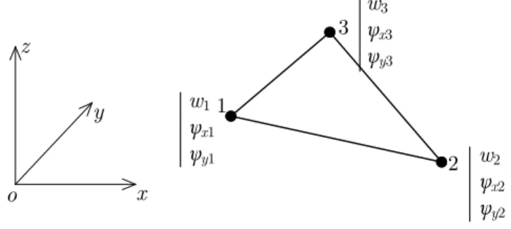
2 THEORETICAL BASIS

2.1 The Mindlin-Reissner Plate Theory

x y z

o

Mxy Tx

Mx My Mxy

Ty

My Mxy

Ty Mxy Tx Mx

x, u z, w

o

∂w/∂x x

y, v z, w

o

∂w/∂y y

Figure 1: Positive directions of displacement components and resultants.

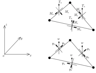
As shown in Figure 1, the positive directions of displacement components and resultants are defined.

The xoy-plane represents the middle surface of Mindlin plate, and the z-axis represents the direction

of thickness (the thickness is denoted by h).

In the mid-surface of Mindlin plate, the transverse deflection along z-axis is denoted by w, and

the rotations of normal vector in xoz-plane and yoz-plane are denoted by x and y, respectively.

Obviously, the deflection w, the rotation x, and the rotation y are all functions of x and y. And the

( , , ) ( , )

( , , ) ( , ) ( / 2 / 2)

( , , ) ( , )

x

y u x y z z x y

v x y z z x y h z h w x y z w x y

y y

ìï =

-ïïï _{= - - £ £}

íï

ï ₌

ïïî

(1)

As the deflection and rotations are independently defined, the rotations x and y are no more

equal to the rotations of mid-surface. The transverse shear strain vector is determined by the differ-ence of the two aforementioned kinds of rotations.

x x y y w x w y y g g _y ì ü

ï ¶ ï

ï _- ï

ï ï

ì ü

ï ï _{ï ï}

ï ï ï ¶ ï

=í_ï ý_ï=í_ï¶ ý_ï

ï ï ï ï

î þ _ï - _ï

ï¶ ï

ï ï

î þ

(2)

From the displacements given in equation (1), the strains paralleled with the xoy-plane at

arbi-trary point in Mindlin plate can be obtained:

ε= x xx x y yy y xy xy y x x

z z z

y

y x

y

e k _y

e k

g k _{y y}

ì ü

ï ¶ ï

ï _- ï

ï ï

ï _¶ ï

ì ü ì ü ï ï

ï ï ï ï _{ï ï}

ï ï ï ï _{ï ¶ ï}

ï ï ï ï _{ï ï}

ï ï_{= =} ï ï₌ ï _- ï

í ý í ý í ý

ï ï ï ï ï ¶ ï

ï ï ï ï ï ï

ï ï ï ï ï ï

ï ï ï ï ï ¶ ï

î þ î þ _ï ¶ _ï

ï- - ï

ï ï

ï ¶ ¶ ï

ï ï

î þ

(3)

where is the curvature vector. And from equations (2) and (3), the strain compatibility equations can be derived:

1 1 2 2 1 1 2 2 xy y x x

y xy x y

y x x y x

x y y y x

k g

k g

k k g g

ì _¶ æ _¶ ö

ï ¶ ¶ ç¶ ÷

ï _{- = ç - ÷}

ï _ç ÷

ï_{¶ ¶ ¶ ç ¶ ¶} ÷_÷

ï è ø

ïí _{æ ö}

ï ¶ ¶ ¶ ç¶ ¶ ÷

ï _{ç ÷}

ï - = _ç - _÷

ï _ç ÷_÷

ï ¶ ¶ ¶ _è ¶ ¶ _ø

ïî

(4)

The bending moments, twisting moment, and shear forces are denoted by Mx, My, Mxy, Tx, and

Ty, respectively, as shown in Figure 1. And the equilibrium equations for a plate under transverse

distributed load q are:

0 0 0 xy x x xy y y y x M M T x y M M T x y T T q x y ì ¶ ï ¶

ï _{+ - =}

ïï ¶ ¶

ïï

ï ¶ ¶

ïï _{+ - =}

íï ¶ ¶

ïï

ï ¶ ¶

ïï + + =

ïï ¶ ¶

ïî

(5)

As shown in Figure 2, Mn, Ms, and Tn denote the bending moment, twisting moment, and shear

force along boundary, respectively; n, s, and w denote the boundary rotations and deflection,

x y z o w w w Tn Tn Tn Mn Mn Mn n n n Ms Ms Ms ψs s s

Figure 2: Positive directions of boundary resultants and displacement components.

The relations between the domain and the boundary resultants, as well as the relations between the domain and the boundary displacement components, are given by

2 2

T

2 2

2 0 0

0 0

0 0 0

x

y n

xy

s x y xy x y

x n

y M

l m lm M

M

M

M lm lm l m M M M T T

T

T l m

T

ì ü

ï ï

ï ï

ï ï

é ù ï ï

ì ü

ï ï _{ê úï ï}

ï ï _{ï ï}

ï ï _{ê úï ï}

ï ï_{= - -} ï ï₌ é ù

í ý ê úí ý _{êë úû}

ï ï _{ê ú}ï ï

ï_- ï _{- -} ï ï

ï ï ê úï ï

ï ï ï ï

î þ ë _{û ïï ïï}

ï ï ï ï î þ L ₍₆₎ n x s y l m m l y y y y

ì ü é ù ì ü

ï ï ï ï

ï ï₌ ê úï ï

í ý _{ê ú}í ý

ï ï _ê- _úï ï

ï ï ï ï

î þ ë û î þ (7)

where l and m are the direction cosines of the boundary’s outer normal.

The constitutive equations for isotropic and linearly elastic Mindlin-Reissner plates with uniform thickness are:

,

b s

= =

M D T D ₍₈₎

where M, T, Db,and Ds are the bending moment vector, shear force vector, bending elasticity matrix,

and shear elasticity matrix, respectively;

, x x y y xy M T M T M ì ü ï ï

ï ï _{ì üï ï}

ï ï

ï ï ï ï

=í_ï ý_ï =í ý_{ï ï}

ï ï ï ïî þ

ï ï

ï ï

î þ

1 0

1 0

1 0 ,

0 1 1

0 0

2

b D s C

m m

m

é ù

ê ú

ê ú _{é ù}

ê ú _{ê ú}

= ê ú = _{ê ú}

ê _- ú _{êë úû}

ê ú

ê ú

ê ú

ë û

D D ₍₁₀₎

(

)

3_{/ 12 1} 2 _{, 5 / 6}

D =Eh é_êë -m ù_úû C = Gh for rectangular sections ₍₁₁₎

in which E, G, and μ are the Young’s modulus, shear modulus, and Poisson’s ratio, respectively; and

h is the thickness of the plate.

Generally, the boundary conditions (BCs) are classified into four categories: 1) Fixed boundary

(S1) condition: deflection and rotations of the boundary are given; 2) ‘Soft’ simply supported (SS1)

condition: deflection, bending moment and twisting moment of the boundary are given; 3) ‘Hard’

simply supported (SS2) condition: deflection, bending moment and rotation s of the boundary are

given; and 4) Free boundary (S3) condition: all the boundary resultants are given.

2.2 The Modified Principle of Complementary Energy for Mindlin-Reissner Plate

The standard complementary energy functional for Mindlin-Reissner plate is given below (Hu, 1984):

T T _d 1 2 u n s C n n s S M d s T M A w y y W ì ü ï ï ï ï ï ï ï ï

P = + í_ï ý_ï

ì ü ï ï ï ï ï ï ï ï ï ï í ý ï ï ï ï ï ï ï ï ï ï î þ

ï_- ï

ï ï

ï ï

î þ

òò

ò

in which yn, ys, and w denote the given boundary displacement components on the displacement

boundary Su; Ω denotes the whole mid-surface region of the plate; C and R denote the elasticity

matrix of compliances and the resultant vector, respectively;

2 2

2 2

1

1

0 0 0

(1 ) (1 )

1

0 0 0

(1 ) (1 )

2

0 0 0 0

(1 )

1

0 0 0 0

1

0 0 0 0

b s D D D D D C C m m m m m m m

-é _- ù

ê ú

ê _{- -} ú

ê ú

ê - ú

ê ú

ê _{- -} ú

ê ú

é ù _{ê ú}

ê ú _{= ê ú}

ê ú _{ê ú}

ê ú

-ë û _{ê ú}

ê ú ê ú ê ú ê ú ê ú ê ú ë û D 0 C =

0 D (13)

T x y xy x y

M M M T T

é ù

= ê_ë ú_û

R (14)

Assume that the region _Ω is divided into several subregions (triangles) Te (e=1~N). And the given

use of the principle of minimum complementary energy, extra constrains should be imposed. Accord-ing to the generalized variational principle, such extra constrains can be imposed by the so-called Lagrange multiplier method.

Extra constrains include the equilibrium conditions on the common boundaries of subregions and

the force boundary conditions on the boundary of _Ω, which are expressed by:

1 2

n n

s s e

n n

M M

M M S

T T

on

ì ü ì ü

ï ï ï ï

ï ï ï ï

ï ï ï ï

ï ï ₌ ï ï

í ý í ý

ï ï ï ï

ï_- ï ï ï

ï ï ï ï

ï ï ï ï

î þ î þ

å

where ΣSe denotes the common boundaries of subregions; the indexes 1 and 2 denote the two

subre-gions that share a common boundary;

n s s n n n M

M on S

T _T M M _s ì ü ï ï ì ü

ï ï ï ï

ï ï ï ï

ï ï ï ï

ï ï₌ï ï

í ý í ý

ï ï ï ï

ï_- ï ï ï

ï ï ï_- ï

ï ï ï ï

î þ _{ïî ïþ}

(16)

where Sσ denotes the force boundary; Mn, Ms , and T n represent the given boundary resultants.

By multiplying the two constrains by corresponding Lagrange multipliers and adding them into the standard complementary energy functional (equation (12)), the modified functional can be ob-tained: T T T T 1 2 1 2 1 2 1 2 1 d d 2 d d u e n n

C s s

S n

n n n

s s s

S S n n s n n n M

M s A

T w

M M

M M

M M s M M s

T T s T T

y y

W

ì ü ì ü

ï ï ï ï

ï ï ï ï

ï ï ï ï

ï ï ï ï

P = í_ï ý í_{ï ï} ý_ï +

ï_- ï ï ï

ï ï ï ï

ï ï ï ï

î þ î þ

ì ü

ì ü ï ï

ï - ï ï - ï

ï ï _{ï ï}

ï ï _{ï ï}

ï ï

ï ï ï ï

+ í_ï - ý_ï + í_ï - ý_ï

ï ï ï ï

ï ï ï ï

å _ïïî + _{ïïþ ïïî}- + _ïïþ

ò

òò

ò

ò

R CR

(17)

where λ1 and λ2 are Lagrange multipliers.

Let the variation of equation (17) be zero:

(

)

1 2 1 2

1 2 1 2

1

1 2 1 2

d d d

d + u e n n s s S S n

n n n n

s s s s

S

n n n

C

n M

s M s A

w T

M M M M

M M s M M

T T T T

s

y d

d d y d d

d

d d

d d

d d

ì ü ì ü

ï ï ï ï

ï ï ï ï

ï ï ï ï

ï ï ï ï

P = í_ï ý_ï + í_ï ý_ï +

ï ï ï_- ï

ï ï ï ï

ï ï ï ï

î þ î þ

ì ü ì ü

ï - ï ï - ï

ï ï ï ï

ï ï ï ï

ï ï ï ï

ï ï ï ï

+ í_ï - ý_ï í_ï - ý_ï

ï ï ï ï

ï ï ï

å _ïïî + _{ïïþ ïïî} + _þ

ò

ò

òò

ò

L R R C R

T T

1d 2d =0

e n s S S n n n s M M

s M M s

T T

s

d d

ì ü

ï _- ï

ï ï

ï ï

ï ï

ï ï

+ í_ï - ý_ï

ï ï

ï ï ï

å

ò

ò

Considering the following constitutive equation:

T

0 1 0

0 0 1

0 0 0

x x y y x y y x w w x y y y y y

é ¶ ¶ ù

ê- - - ú

ê _{¶ ¶} ú _{ìï üï ìï üï}

ê ú ï ï ï ï

ì ü

ï ï ê ¶ ¶ ú ï ï ï ï

ï ï_{= ê - - - ú} ï ï₌ ï ï

í ý í ý í ý

ï ï ê ¶ ¶ ú ï ï ï ï

ï ï ï ï ï ï

î þ _{ê ú ï ïï ï ï ï}

ï ï

¶ ¶ î þ î þ

ê ú

ê _{¶ ¶} ú

ê ú

ë û

F = CR (19)

where F is an operator matrix, the area integral in equation (18) can be simplified. Integrate by parts

for the area integral, we obtain

Ω

T T

T _d T _d T _d

e e

x x

y y

e T T

A A s

w w

y y

d y d y d

¶

æ _{ì ü ì ü} ö_÷

ç ï ï ï ï _÷

ç ï ï ï ï _÷

ç ï ï ï ï ÷

ç ï ï ï ï ÷

= ç_ç í ý_{ï ï} + í ý_{ï ï} ÷_÷

÷

ç _{ï ï ï ï ÷}

ç _{ï ï ï ï ÷}

ç _{ï ï ï ï ÷}

ç î þ î þ

è ø

òò

å

òò

ò

in which

F



the boundary of the e-th subregion;

T

T

0 1 0

0 0 0

0 0 1 , 0 0 0

0 0 0

0 0 0

x y _{l m}

m l

y x

l m

x y

é _{¶ ¶} ù

ê - ú

ê_{¶ ¶} ú _{é- - ù}

ê ú _{ê ú}

¶ ¶

ê ú _{ê ú}

= ê - ú = _ê - - _ú

ê ¶ ¶ ú _{ê ú}

ê _{¶ ¶} ú _{êë úû}

ê _{- -} ú

ê _{¶ ¶} ú

ê ú

ë û

F n (21)

where l and m are still the direction cosines of boundary’s outer normal.

Because the trial functions of resultants satisfy the equilibrium equations in each subregion, var-iation of equations (5) yields following result:

T_{d =0}

F R (22)

Thus, equation (18) can be simplified as

(

)

(

)

T _{1 2}

1 1 T 2 d d + d e u x n y s

e T S

n n n n s s C s S n n M

s M s

w T

M M

s M M

w T T

s

y d

d d y d

d

d d

y

d y d d

d d

¶

æ ìï üï ö_÷ ìï üï

ç ï ï _÷ ï ï

ç ï ï ÷ ï ï

ç ï ï ÷ ï ï

ç

P = _ç í_ï ý_ï ÷_÷+ í_ï ý_ï

ç _{ï ï} ÷_{÷ ï ï}

ç _{ï ï ÷ ï- ï}

çè ïî ïþ ø ïî ïþ

ì ü

ì ü ï - ï

ï ï _{ï ï}

ï ï _{ï ï}

ï ï _{ï ï}

ï ï ₊ ï _- ï

í ý í ý

ï ï ï ï

ï ï ï ï

ï ï ï + ï

ï ï ï ï

î þ ïî ïþ

ò

ò

å

ò

n R

L R d 0

e

S

s =

å

ò

(23)

T

0 0

0 0 1

l m m l

é ù

ê ú

ê_- ú ₌

-ê ú

ê ú

ê ú

ë û

n L ₍₂₄₎

equation (23) can be further simplified to be

T

T _{1 2}

1 2 2 1 1 2 2 d n n

n n n

s s s s s

S n C n n M M M

M s M M

T w T T w

s

d d

d y y

d d y d d y

d d d

ì ü

ì ü ì ü ï - ï ì ü

ï ï ï ï _{ï ï} ï ï

ï ï ï ï _{ï ï} ï ï

ï ï ï ï _{ï ï} ï ï

ï ï ï ï ï ï ï ï

P = í_ï ý_ï í_ï ý_ï + í_ï - _ïý _ïí ý_ï

ï_- ï ï ï ï ï ï ï

æ ö

æ ö_{÷ ç ÷}

ç _{÷ ç ÷}

ç

ï ï ï ï ï + ï ï ï

ï ï ï ï

÷

÷ ç

ç ÷ _ç ÷

ç - ÷ _ç + ÷

ç ÷ _ç ÷_÷

ç ÷_{÷ ç ÷}

ç _{÷ ç}

ç _{ï ï} ç _{ï ï}

î þ è î þø ïî ïþ è î þ ø

ò

e S s å ÷÷ =

ò

Due to the arbitrariness of variation about resultants R, it can be easily concluded that the

Lagrange multipliers are just (boundary) displacement components on corresponding boundaries. Fi-nally, the modified functional of complementary energy can be fully determined:

T T

T

1

d d + d

2

e e ue e e

n n n

s s s

e S S S e e

n S n n C T s M M

M s M s A

T w _T w

s s y y y y + + ì ü ï ï

ì ü ì ü ì ü

ï ï ï ï ï ï ï ï

ï ï ï ï ï ï ï ï

ï ï ï ï ï ï ï ï

ï ï ï ï ï ï ï ï

P = í_ï ý í_{ï ï} ý_ï - í_ï ý í_{ï ï} ý_ï

ï_- ï ï ï ï ï ï ï

ï ï ï ï ï- ï ï ï

ï ï ï ï ï ï ï ï

î þ î þ _{ïî ïþ} î þ

ò

ò

òò

å

å

å

2.3 The Displacement Function of Mindlin-Reissner Plate

Hu (1984) proposed the so-called displacement functions F and f for Mindlin-Reissner plates, from

which the displacement components can be derived theoretically.

For a plate loaded by distributed transverse force q, the displacement components are given as

2

, ,

x y

F f F f D

w F F

x y y x C

y = ¶ + ¶ y = ¶ -¶ = - 

¶ ¶ ¶ ¶ (26)

where D and C are bending stiffness and shear stiffness mentioned in equation (11), respectively. The

functions F and f satisfy the following differential equations.

2 2

D

 

F

=

q

(

)

1 0

2 -m D -f Cf = (28)

It should be noted that equation (27) is quite similar to the governing equation of the deflection

for thin plates under Kirchhoff’s assumption. In fact, Hu pointed out that function F even satisfies

the same boundary conditions as the deflection of thin plates if the plate is thin enough. Function f

represents the influence of shear deformation, and describes the phenomenon of edge effect for Mindlin

plates. In some cases, the function f vanishes, such as simply supported polygonal plates, circular

plates of axial symmetry and other cases in which the shear forces are statically determinate (Hu,

higher-order elements, the influence of displacement function f must be taken into account, otherwise the elements may present poor results for stress and strain, even for nodes away from the boundary (Bao et al., 2017).

Substitution of equation (26) into equations (2) and (3) yields

2 2 2 2 2 2 2 2 ( ) ( ) x y xy x y F x F y F x y D F C x D F C y k k k g g ì ü

ï ¶ ï

ï _- ï

ï ï

ï ï

ï ¶ ï

ï ï

ï ï

ì ü ¶

ï ï ï ï

ï ï ï - ï

ï ï ï ï

ï ï ï _¶ ï

ï ï ï ï

ï ï ï ï

ï ï ï ï

ï ï₌ï ¶ ï

í ý í _- ý

ï ï ï ï

ï ï ï ¶ ¶ ï

ï ï ï ï

ï ï ï _¶ ï

ï ï ï ï

ï ï ï_{- } ï

ï ï ï ï

ï ï

î þ ï_ï ¶ ï_ï

ï _¶ ï

ï ï

ï-  ï

ï ï

ï ¶ ï

ï ï

î þ

(29)

Then, substitution of equation (29) into the constitutive equations (8) yields

2 2 2 2 2 2 2 2 2 2 2 (1 ) ( ) ( ) x y xy x y F F x y F F M

M y x

F M D x y T T F x F y m m m ì ü

ï¶ ¶ ï

ï ₊ ï

ï ï

ï ï

ï¶ ¶ ï

ï ï

ï ï

ì ü ï¶ ¶ ï

ï ï _{ï ï}

ï ï _{ï + ï}

ï ï _{ï ï}

ï ï _{ï¶ ¶ ï}

ï ï _{ï ï}

ï ï _{ï ï}

ï ï

ï ï ï _¶ ï

=í_ï ý_ï= - í_{ï -} ý_ï

ï ï ï ¶ ¶ ï

ï ï ï ï

ï ï ï ï

ï ï ï ¶ ï

ï ï ï _ ï

ï ï ï ï

ï ï

î þ ï_{ï ¶} ï_ï

ï _¶ ï

ï ï

ï _ ï

ï ï

ï _¶ ï

ï ï

î þ

R ₍₃₀₎

It is emphasized that the curvatures, shear strains, and resultants derived from displacement

function F satisfy all governing equations of Mindlin-Reissner plates. Thus, it’s quite reasonable to

gain proper trial functions by means of displacement functions.

Assumed that the distributed transverse force q is constant, then, the displacement function F

can be solved.

0 *

F = F +F (31)

in which F is expressed as the sum of the general and the particular solutions.

Considering the symmetry between x and y axes, the particular solution can be chosen as (other

choices such as * 2 2

8

q

F x y

D

= have been also tested, but the following one is better.)

(

)

* 4 4

48

q

F x y

D

= + (32)

2 2 0 ₀

D  F = (33)

which can be easily solved in polynomial form. The first seven general solutions and corresponding resultants are listed in Table 1. The first order completeness of bending moments and zero order completeness of shear forces are guaranteed. More analytical solutions can be found in reference (Cen et al., 2014).

i 1 2 3 4 5 6 7

0

i DF

- _x2 _{xy y}2 _x3 _x2_{y xy}2 _y3

0

xi M

i

R

2 0 2μ 6x 2y 2μx 6μy

0

yi

M 2μ 0 2 6μ_x 2μ_y 2_x 6_y

0

xyi

M 0 1−μ 0 0 2(1−μ)_x 2(1−μ)_y 0

0

x i

T 0 0 0 6 0 2 0

0

yi

T 0 0 0 0 2 0 6

Table 1: The first seven general solutions of F and corresponding resultants.

2.4 The Locking-free Formulae of Timoshenko’s Beam

wj

i j

i ψj

lij

l r=l/lij wi

Figure 3: Positive directions of displacement components for Timoshenko’s beam.

As shown in Figure 3, in locking-free formulae of Timoshenko’s beam (Hu, 1984), the deflection w,

rotation , and shear strain are assumed to be cubic, quadratic, and constant, respectively, and are given by

(

)

(

)

(

)

(

)

(

)

(

)

(

)

(

)

3 3 2 3

2 3

2 2 2

2

1 1 2 1 2 1 2

2

1 2

2

6 6

1 2 1 2 1 3 1 2

3 1 2

ij

ij i ij j ij i

ij

ij j

ij i ij j i

i

j i

ij ij

i j

j

j

l

w r F w r F w F F

l

F F

F w F w r F

l l

r F

d d d y

d y

y d d

g

y

d

d

d y

ìïï _{= é - + - ù +é - - ù é + - ù}

ïï ë û ë û ë û

ïï

ïï _{é ù}

ï -

-ï _{ë û}

ïï

ïï _{= - - + - é - - - ù}

í _{ë û}

ïï

ïï _{é - - ù}

ï _{ë û}

ïï ï

+

-+

+

ïï G

î = ïï ïï

(34)

(

)

(

)(

)

(

) (

)

2 1 , 3 1 1 2 , ₂

6 ₂

, ( )

1 12

, ij j i j i ij

ij

ij

ij i j i j

ij ij

D

F r r F r r r l x x y y

Cl

w w l

l

l

d y y

l

ìïï = - = - - = - + - =

ïï ïï íï

ïï = G = - + -

-ï ₊

ïïî

(35)

Here D and C represent the beam’s bending stiffness and shear stiffness, respectively, and will be

replaced by corresponding stiffness of Mindlin plates in the following section.

As discussed in Section 1, the interpolation technique based on the formulae of Timoshenko’s beam has been successfully applied in many effective elements (Soh et al., 1999).

3 FORMULAE OF THE NEW ELEMENT HDF-P3-7

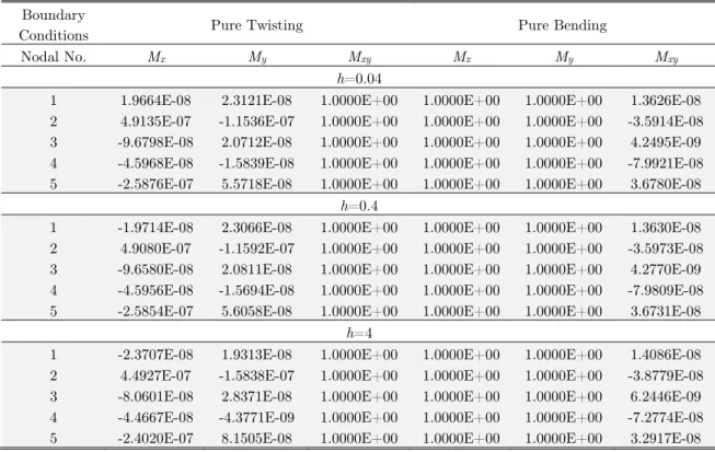
β

Figure 4 shows a 9-DOF triangular plate bending element, and assume that the whole plate Ω is

meshed into several triangles Te (e=1~N).

x y z

o

1

2 3

w2

x2

y2

w3

x3

y3

w1

x1

y1

Figure 4: Nodal DOFs of the 3-node triangular hybrid displacement function element.

Firstly, the assumed resultant fields can be derived from the aforementioned solutions of

displace-ment function F:

* 0

= +

R R R (36)

in which R0 denotes the general solution part, and is taken as a linear combination of the first seven

general solutions of F listed in Table 1:

1

2

1 2

0

7

7 =

b b

b

ì ü ï ï ï ï ï ï ï ï ï ï ï ï

é _¼ ù_{í ý=}

ê ú

ë _{û ï ïï ï}

ï ï ï ï ï ï ï ï î þ

R R R R S

 (37)

where i(i=1~7) are unknown resultant parameters, and Ri (i=1~7) are the resultant vectors derived

from the first seven general solutions of F by employing equation (30), which have been given by

Table 1; R* denotes the particular solution part, andcan be derived directly from the particular

(

)

(

)

ï_{- +} ï

ï ï

ï ï

ï ï

ï ï

ï ï

ï_{- +} ï

ï ï

ï ï

ï ï

ï ï

= í_ï ý_ï

ï ï

ï ï

ï _- ï

ï ï

ï ï

ï ï

ï ï

ï ï

ï - ï

ï ï

ï ï

î þ

R ₍₃₈₎

Thus, the assumed resultants satisfy the equilibrium equations in each subregion Te. So, the

modified functional of complementary energy given in Section 2 can be employed.

Secondly, the displacement components along each element boundary are chosen as the locking-free formulae of Timoshenko’s beam theory.

Substitution of the relations

(

)

(

)

(

)

(

)

s xi xj x yi yj y lij and n yj yi x xi xj y lij

y = -é_ë - y + - y _ûù y = é_ë - y + - y ù_{û (39)}

into equation (34) yields

(

)

(

)

(

)

(

)

(

)

(

)

(

)

(

)

(

)

(

)

(

)

(

)

(

)

1 1 2 1 2

1 1 2 2 1 1 2 2 6 6

1 2 1 2

1

1 3 1 2

1

3 1

ij i ij j

ij i j xi i j yi

ij i j xj i j yj

s ij i ij j

ij ij

ij i j xi i j yi

ij

ij

w r F w r F w

F F x x y y

F F x x y y

F w F w

l l

r F x x y y

l r l

d d

d y y

d y y

y d d

d y y

é ù é ù

= _ë - + - _û +_ë - - _û

é ù é ù

- _ë + - _{û ë} - + - _û

é ù é ù

+ _ë - - _{û ë} - + - _û

= - - +

-é ù é ù

- _ë - - - _{û ë} - + - _û

- _ëé -

(

)

(

)

(

)

(40)

Then, the rotation along normal direction is assumed to be linear function.

(

)

(

)

(

)

(

)

(

)

(

)

1

1 1

1

n ni nj

j i xi i j yi j i xj i j yj

ij ij

r r

r y y x x r y y x x

l l

y y y

y y y y

= - + =

é ù é ù

- _ë - + - _û+ _ë - + - _û (41)

These three complicated equations can be rewritten in the form of matrix:

T

1 1 1 2 2 2 3 3 3

n

s w x y w x y w x y w

y

y y y y y y y

ì ü

ï ï

ï ï

ï ï

ï ï₌ é ù ₌

í ý _{êë úû}

ï ï

ï ï

ï ï

ï ï

î þ

N Nqe

where qe _{is the nodal displacement vector of the}

e-th element, and N is the boundary displacement

interpolation function matrix or shape function matrix.

It is easy to see that the matrices N on different edges are different:

13 15 16

21 22 23 24 25 26

12

31 32 33 34 35 36

12

0 0 0 0 0

0 0 0 0 0 0

N N N

N N N N N N

N N N N

N

N N

é ù

ê ú

ê ú

= ê ú

ê ú

ê ú

ë û

N

15 16 18 19

24 25 26 27 28 29

23

34 35 36 37 38 39

0 0 0 0 0

0 0 0 0 0 0

N N N N

N N N N N N

N N N N N N

é ù

ê ú

ê ú

= ê ú

ê ú

ê ú

ë û

N

12 13 18 19

21 22 23 27 28 29

31

31 32 33 37 38 39

0 0 0 0 0

0 0 0 0 0 0

N N N N

N N N N N N

N N N N N N

é ù

ê ú

ê ú

= ê ú

ê ú

ê ú

ë û

N

(43)

All the non-zero components can be detailed directly from equations (40) and (41).

Thirdly, as the assumed resultants and boundary displacement components are all given, the modified functional of complementary energy can be fully determined.

Let

*

M S CST M* S CRT * T *

T T *T T

d , d , d

d , d

e e e

e e

T T T

T T

A A Q A

s s

¶ ¶

= = =

= =

òò

òò

òò

ò

ò

R CR

H S L N V R L N (44)

then, the modified functional of complementary energy can be simplified as:

(

)

T

1 2

d

e

e e e e e e

C e e e e S n s n Q M M s T s

P = + + + +

æ æ _{ì ü} ö_÷ ö_÷

ç ç ï ï _{÷ ÷}

ç ç ï ï

æ _ö÷ ç _÷ ç _÷ ç ÷ è ÷ ÷

ç ç ï ï ÷ ÷

ç ç ï_ï ï_ï ÷ ÷

ç ç ÷ ÷

+ ç_ç -ç_ç í_ï ý_ï ÷_÷ ÷_÷

÷ ÷

ç ç ï ï _{÷ ÷}

ç ç ï- ï ÷ ÷

ç ç ï ï ÷ ÷

ç ç ïî ïþ ÷ ÷

è è ø ø ø

å

ò

å

M M M Hq

Vq N q

(45)

in which βe denotes the resultant parameter vector of the e-th element. It should be emphasized that

the resultant parameter vectors of different elements are independently defined, so that they can vary independently.

Using the modified principle of complementary energy, the variation of modified functional (45) is taken to be zero:

0, 0

e

C C

e d d

¶ ¶P

¶ ¶

P

= q =

q (46)

* _{( 1 ~ )} e _{+ +} e _{= e= N}

M M Hq 0 ₍₄₇₎

T

T _{d 0}

e n s e e S n M M s T s d

æ _{ì ü} ö_÷

ç ï ï _÷

ç ï ï _÷

ç ï ï ÷

ç ïï ïï ÷

ç _{+ - í ý} ÷ ₌

ç _÷÷

ç ï ï _÷

ç ï ï ÷

ç ï- ï ÷

ç ï ï ÷

ç ïî ïþ ÷

è ø

ò

å

which gives the relation between βe and qe

. It may be found that equation (48) is not so rigorous, and some assembling rules should be discussed.

Equation (47) yields

1₍ * ₎

e _{= -M}- _{M +Hq}e ₍₄₉₎

Substitution of equation (49) into equation (48) yields

(

)

(

)

T

T

1 * _{d 0}

e n s e e S n M M s T s d

-æ _{ì ü} ö_÷

ç ï ï _÷

ç ï ï _÷

ç ï ï ÷

ç ïï ïï ÷

ç _{- + + - í ý} ÷ ₌

ç _÷÷

ç ï ï _÷

ç ï ï ÷

ç ï- ï ÷

ç ï ï ÷

ç ïî ïþ ÷

è ø

ò

å

Above equation gives the discrete global equilibrium equation for this kind of element:

(

)

(

)

T T

T

1 * _d

e e e n s S n M M s T s

-æ _{ì ü} ö_÷

ç ï ï _÷

ç ï ï _÷

ç ï ï ÷

ç ïï ïï ÷

ç _{- + + - í ý} ÷ ₌

ç _÷÷

ç ï ï _÷

ç ï ï ÷

ç ï- ï ÷

ç ï ï ÷

ç ïî ïþ ÷

è ø

ò

å

in which the summation notation means that some assembling rules of element equilibrium equations should be followed. In fact, the assembling rule is the same as what we use in traditional displacement-based element cases, which can be easily found from equation (50).

It should be noted that:

1)The element stiffness matrix is just _{H M H}T -1 _;

T 1

e

-K = H M H (52)

Now it can be explained that why only the first seven general solutions of resultants are employed. To avoid spurious zero energy modes, the rank of single element stiffness matrix should be at least

9₋3=6, which means that at least six general solutions should be included. Completeness requirement

tells us that seven solutions or eleven solutions are reasonable choices, but numerical results show that seven solutions are enough and always achieve higher accuracy.

T T 1 * T _d

e

n

s

S

n e

M

M s

T

s

-ì ü

ï ï

ï ï

ï ï

ï ï

ï ï

= - í_ï ý_ï

ï ï

ï_- ï

ï ï

ï ïþ

-î

ò

P V H M M N ₍₅₃₎

In above equation, (_VT _{-H M M}T -1 *_{) denotes the equivalent nodal forces of body forces, and}

the last part denotes the equivalent forces of boundary forces.

Then, the element equilibrium equation can be written as

_P

_-

_{K q}

₌

₀

the assembled global equilibrium equation. It is surprising but reasonable that the equivalent forces of boundary forces possess the same form as displacement-based elements.

3) The assembling rules of hybrid displacement function elements are consistent with traditional displacement-based elements. So it can be easily integrated into the standard framework of finite element programs.

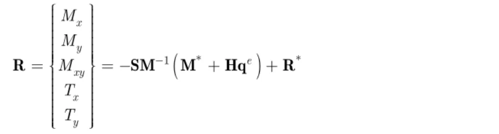
Boundary

Conditions Pure Twisting Pure Bending

Nodal No. Mx My Mxy Mx My Mxy

h=0.04

1 1.9664E-08 2.3121E-08 1.0000E+00 1.0000E+00 1.0000E+00 1.3626E-08

2 4.9135E-07 -1.1536E-07 1.0000E+00 1.0000E+00 1.0000E+00 -3.5914E-08

3 -9.6798E-08 2.0712E-08 1.0000E+00 1.0000E+00 1.0000E+00 4.2495E-09

4 -4.5968E-08 -1.5839E-08 1.0000E+00 1.0000E+00 1.0000E+00 -7.9921E-08

5 -2.5876E-07 5.5718E-08 1.0000E+00 1.0000E+00 1.0000E+00 3.6780E-08

h=0.4

1 -1.9714E-08 2.3066E-08 1.0000E+00 1.0000E+00 1.0000E+00 1.3630E-08

2 4.9080E-07 -1.1592E-07 1.0000E+00 1.0000E+00 1.0000E+00 -3.5973E-08

3 -9.6580E-08 2.0811E-08 1.0000E+00 1.0000E+00 1.0000E+00 4.2770E-09

4 -4.5956E-08 -1.5694E-08 1.0000E+00 1.0000E+00 1.0000E+00 -7.9809E-08

5 -2.5854E-07 5.6058E-08 1.0000E+00 1.0000E+00 1.0000E+00 3.6731E-08

h=4

1 -2.3707E-08 1.9313E-08 1.0000E+00 1.0000E+00 1.0000E+00 1.4086E-08

2 4.4927E-07 -1.5838E-07 1.0000E+00 1.0000E+00 1.0000E+00 -3.8779E-08

3 -8.0601E-08 2.8371E-08 1.0000E+00 1.0000E+00 1.0000E+00 6.2446E-09

4 -4.4667E-08 -4.3771E-09 1.0000E+00 1.0000E+00 1.0000E+00 -7.2774E-08

5 -2.4020E-07 8.1505E-08 1.0000E+00 1.0000E+00 1.0000E+00 3.2917E-08

Table 2: Results for patch tests.

The integrals in equation (44) are all calculated by numerical integration methods. One dimen-sional Gauss integration and Hammer integration schemes are employed. As the integrands are pol-ynomials, all the integrals can be calculated exactly. In this paper, four integration points are em-ployed for both line integrals and area integrals in equation (44), and it can be sure that the results are all accurate.

Following the aforementioned steps, the global nodal displacement components can be solved.

(

)

1 * *

x

y

e xy

x

y M

M M T

T

-ì ü

ï ï

ï ï

ï ï

ï ï

ï ï

ï ï

ï ï

ï ï

=í_ï ý_ï= - + +

ï ï

ï ï

ï ï

ï ï

ï ï

ï ï

ï ï

î þ

R SM M Hq R ₍₅₄₎

the resultants at arbitrary point of the element can be obtained. Furthermore, the resultants at any nodes can be taken as the average value of different elements.

BCs Thickness 2×2 4×4 8×8 16×16 Reference

SS2

Deflection

h=0.001 0.9876 0.9974 0.9994 0.9999

1.0000

h=0.1 0.9914 0.9971 0.9991 0.9998

Bending Moment

h=0.001 0.9569 0.9815 0.9931 0.9975

1.0000

h=0.1 0.9568 0.9867 0.9962 0.9988

S1

Deflection

h=0.001 0.9681 0.9915 0.9987 1.0000

1.0000

h=0.1 0.9970 1.0019 1.0017 1.0031

Bending Moment

h=0.001 1.0768 0.9937 0.9959 0.9982

1.0000

h=0.1 1.0191 1.0070 1.0046 1.0043

Table 3: Normalized central deflection and bending moment results of the proposed element.

Once the stiffness matrix for static analysis is derived, what we need to extend the proposed element into free vibration analysis of Mindlin plate is the formulae of inertia matrix. Considering the corresponding variational principles for free vibration problems, hybrid element method can be extended into the analysis of free vibration problems theoretically. But as we mentioned in Section 1, such scheme does not give the formulae of inertia matrix and a nonlinear eigenvalue problem has to be solved.

Actually, some inertia matrices of displacement-based elements can cooperate well with the stiff-ness matrix of the proposed element in analyzing the free vibration of plate structures. And the diagonal inertia matrix of the 3-node triangular isoparametric element is almost the best choice, for both convergence property and computational cost. Thus, though no rigorous mathematical proof has been given yet, the generalized eigenvalue equation is still given by

(

)

2

3 3

/ 3 0 0

, , 0 / 36 0

0 0 / 36

e

e e e

i e

Ah

Ah

Ah r

w r

r

é ù é ù

ê ú ê ú

ê ú ê ú

- = = _{ê ú} = _{ê ú}

ê ú ê ú

ê ú ê_ë ú_û

ë û

M 0 0

K M q 0 M 0 M 0 M

0 0 M

(55)

where ρ is the density of the plate, A is the area of the e-th element and is the natural frequency.

the subspace iteration method (Bathe and Wilson, 1973), and the frontal method is also employed in computer coding for saving computer memory (Liu, 1989).

4 NUMERICAL EXAMPLES

Several standard numerical examples are employed in this section to test the performance of the

proposed element HDF-P3-7. And results obtained by following models are also given for comparison.

DKT: Triangular discrete Kirchhoff element proposed by Batoz et al. (1980).

DKTM, RDKTM: Refined triangular Mindlin plate elements proposed by Chen et al. (2001). DST-BL: A compatible triangular Mindlin plate element based on the discrete shear triangle technique proposed by Batoz et al. (1989).

DST-BK: An incompatible triangular Mindlin plate element based on the discrete shear triangle technique proposed by Batoz et al. (1992).

Mesh 2×2 4×4 8×8 16×16 Reference

wC/wref

HDF-P3-7β 0.9050 0.9736 0.9899 0.9941

1.0000

DKT 0.8045 0.9474 0.9845 0.9947

ARS-T9 0.7964 0.9488 0.9838 0.9926

MiSP3 0.7218 0.9314 0.9824 0.9936

MiSP3+ 0.7823 0.9578 0.9893 0.9942

MITC4 0.4853 0.8419 0.9515 0.9814

DKTM - 0.9474 0.9919 -

RDKTM - 0.9474 0.9919 -

THS 0.9093 0.9692 0.9878 -

My/Mref

HDF-P3-7β 0.9305 0.9913 0.9999 1.0008

DKT 0.9336 1.0000 1.0007 1.0009

ARS-T9 0.9537 0.9969 1.0012 1.0012

MiSP3 0.6954 0.9313 0.9974 0.9981

MiSP3+ 0.7057 0.9490 0.9908 0.9992

MITC4 0.3940 0.8036 0.9459 0.9878

Table 4: 60° skew plate: Normalized deflection and bending moment at point C.

MITC4: A quadrilateral Mindlin-Reissner plate element based on a mixed interpolation scheme proposed by Bathe et al. (1985).

THS: A triangular hybrid stress element based on analytical solutions of thin plate equations proposed by Rezaiee-Pajand et al. (2014).

ARS-T9: A triangular Mindlin plate element based on the improved shear strain interpolation derived from the locking-free Timoshenko’s beam element proposed by Soh et al. (1999).

T3BL, T3BL(R): Triangular Mindlin plate elements based on the linked interpolation method proposed by Taylor and Auricchio (1993).

MiSP3: Hybrid-mixed Mindlin plate elements based on the mixed shear projected method pro-posed by Ayad et al. (1998).

NS+ES-FEM: A ‘hybrid’ smoothed element proposed by Wu et al. (2014).

MIN3: A 3-node Mindlin plate element with improved transverse shear proposed by Tessler et al. (1985).

DSG3: Mindlin plate element based on the discrete shear gap method proposed by Bletzinger et al. (2000).

NS-DSG3, ES-DSG3: Two smoothed Mindlin plate elements of the smoothed FEM family pro-posed by Liu et al. (2009a, 2009b).

S4R, S3R: The quadrilateral and triangular shell elements assembled in the renowned commercial FEM software Abaqus (2009).

4.1 Numerical Examples: Static Analyses

4.1.1 Patch Tests

As shown in Figure 5, a patch is divided by four elements. Three kinds of thickness are considered. Proper constrains are imposed to eliminate rigid body motions. The size and constants are also given in the figure. Both pure bending boundary forces and pure twisting boundary forces are tested, and these two cases are shown in Figure 6.

E=1000.0

μ=0.3 h=0.4, 0.04, 4

1 2

3

4 5

40 20

30

15

Figure 5: Patch tests: Geometry and mesh type.

Mx=My=0

Mxy=1 Ms=1

Ms=1

Ms=1

Ms=1 Mx=My=1

Mxy=0 Mn=1

Mn=1

Mn=1

Mn=1

Figure 6: Pure twisting and pure bending boundary conditions.

Mesh 2×2 4×4 8×8 16×16 Reference

wO/(qL4/1000D)

HDF-P3-7β 1.4473 1.1103 1.0348 1.0225

1.0000

NS+ES-FEM - 1.2049 1.0907 1.0554

ARS-T9 1.5338 1.1096 1.0397 1.0277

MIN3 - 0.6681 0.7600 0.8493

DSG3 - 0.6400 0.6507 0.7718

T3BL 1.3164 1.0316 1.0179 1.0137

T3BL(R) 1.7939 1.1978 1.0752 1.0449

DKT - 1.1103 1.0392 1.0270

DKTM - 0.8750 0.8309 0.8652

RDKTM - 1.1103 1.0392 1.0270

THS - 1.0368 1.0000 1.0000

Mmax/(qL2/100)

HDF-P3-7β 1.0914 1.0727 0.9971 1.0113

NS+ES-FEM - 1.0397 1.0397 1.0185

ARS-T9 1.4763 1.1605 1.0382 1.0215

MIN3 - 0.6542 0.7970 0.8855

DSG3 - 0.6499 0.6840 0.7949

T3BL 0.7540 0.9019 0.9910 1.0012

T3BL(R) 0.7579 0.9528 1.0012 1.0171

Mmin/(qL2/100)

HDF-P3-7β 0.5742 1.0953 0.9328 1.0213

ARS-T9 1.7886 1.3234 1.0331 1.0407

T3BL 0.6937 0.8846 1.0097 1.0188

T3BL(R) 0.7589 0.8931 1.0177 1.0415

Table 5: 30° skew plate: Normalized deflection and principal bending moments at point O.

4.1.2 Square Plate Loaded by Uniform Distributed Transverse Load

x y

o _y=0

x=0

Figure 7: Typical mesh employed for a quarter of plate.

As shown in Figure 7, due to the symmetry, only a quarter of plate is calculated. Clamped boundary condition and hard simply supported boundary condition are considered. The span, distributed

trans-verse force, bending stiffness, Poisson’s ratio, and thickness of the plate are denoted by L, q, D, μ,

and h, respectively, and are given by

L=1, q=1, D=1, μ=0.3, h=0.001, 0.1.

4 2

/ , /

100 10

c c c c

qL qL

w w M M

D

æ ö_÷ æ ö_÷

ç _÷ ç _÷

= ç_{ç ÷÷} = ç_{ç ÷÷}

÷ ÷

ç ç

è ø è ø (56)

calculated by the proposed element, which are compared with the reference solutions (Taylor and Auricchio, 1993), are listed in Table 3. Comparisons with results obtained by other elements are plotted in Figure 8 and Figure 9. From these results, it can be concluded that the proposed

HDF-P3-7 element shows better convergence in most of square plate cases.

Number of Elements (N) 6 24 96 384 Reference

wc/wref

h=0.1

HDF-P3-7β 1.0282 1.0074 1.0019 1.0005

1.0000

ARS-T9 0.9502 0.9894 0.9991 0.9993

T3BL(R) 1.0599 1.0158 1.0028 0.9993

T3BL 0.9900 0.9931 0.9988 0.9997

DST-BK 0.9387 0.9850 0.9962

-DST-BL 0.9502 0.9891 0.9974

-DKT 0.9498 0.9886 0.9971

-DKTM 0.7877 0.9611 0.9935

-RDKTM 0.9502 0.9890 0.9975

-h=1

HDF-P3-7β 1.0233 1.0058 1.0014 1.0003

ARS-T9 0.9486 0.9879 0.9991 0.9992

T3BL(R) 1.0554 1.0150 1.0038 1.0010

T3BL 0.9895 0.9959 0.9989 0.9998

DST-BK 0.9348 0.9838 0.9965

-DST-BL 0.9900 0.9985 1.0025

-DKTM 0.9219 0.9827 0.9961

-RDKTM 0.9486 0.9877 0.9970

-Mc/Mref

Number of Elements (N) 6 24 96 384

h=0.1

HDF-P3-7β 1.0294 1.0086 1.0029 1.0008

ARS-T9 1.0205 1.0199 1.0077 1.0021

T3BL(R) 0.9209 0.9771 0.9933 0.9976

T3BL 0.9131 0.9757 0.9938 0.9985

DST-BK 1.0531 1.0240 1.0085

-DST-BL 1.0201 1.0143 1.0046

-DKT 1.0199 1.0091 1.0050

-DKTM 0.7455 0.9831 1.0025

-RDKTM 1.0199 1.0093 1.0052

-h=1

HDF-P3-7β 1.0203 1.0070 1.0030 1.0010

ARS-T9 1.0343 1.0221 1.0103 1.0032

T3BL(R) 0.9204 0.9763 0.9938 0.9985

T3BL 0.9161 0.9754 0.9937 0.9985

DST-BK 1.0221 1.0124 1.0046

-DST-BL 1.0279 1.0182 1.0124

-DKTM 1.0465 1.0182 1.0093

-RDKTM 1.0290 1.0160 1.0087

4.1.3 Skew Plates Loaded by Uniform Distributed Transverse Load

Razzaque’s 60° plate

As shown in Figure 10, a 60° skew plate with two free and two soft simply supported edges was firstly used by Razzaque (1973) to test the accuracy of thin plate elements, and it has been treated as a classical benchmark for both thin and thick plate elements. The edge length, transverse force,

thick-ness, Young’ modulus, and Poisson’s ratio are denoted by L, q, h, E, and μ, respectively, and are

given by

L=100, q=1, h=0.1, E=10.92, μ=0.3.

For the central deflection wC and bending moment My at point C, Razzaque (1973) give out the

finite difference solutions:

9 3

ref 0.7945 10 , ref 0.9589 10

w = ´ M = ´ ₍₅₇₎

Figure 9: Clamped boundary case: the plate central deflection and bending moment results.

x y

A B

C

D E

Figure 10: A 60° skew plate: Geometry and mesh type.

Results obtained by different elements are listed in Table 4 and plotted partly in Figure 11. It can be easily concluded that the proposed element gives almost the best solutions for both deflection and bending moment.