Prediction of Pathological Stage in Patients
with Prostate Cancer: A Neuro-Fuzzy Model
Georgina Cosma1☯*, Giovanni Acampora1‡
, David Brown1‡, Robert C. Rees2, Masood Khan3☯, A. Graham Pockley2☯
1Computing and Technology, School of Science and Technology, Nottingham Trent University, Nottingham, United Kingdom,2John van Geest Cancer Research Centre, Nottingham Trent University, Nottingham, United Kingdom,3Department of Urology, University Hospitals of Leicester NHS Trust, Leicester, United Kingdom
☯These authors contributed equally to this work. ‡These authors also contributed equally to this work.
*georgina.cosma@ntu.ac.uk
Abstract
The prediction of cancer staging in prostate cancer is a process for estimating the likelihood that the cancer has spread before treatment is given to the patient. Although important for determining the most suitable treatment and optimal management strategy for patients, staging continues to present significant challenges to clinicians. Clinical test results such as the pre-treatment Prostate-Specific Antigen (PSA) level, the biopsy most common tumor pattern (Primary Gleason pattern) and the second most common tumor pattern (Secondary Gleason pattern) in tissue biopsies, and the clinical T stage can be used by clinicians to pre-dict the pathological stage of cancer. However, not every patient will return abnormal results in all tests. This significantly influences the capacity to effectively predict the stage of pros-tate cancer. Herein we have developed a neuro-fuzzy computational intelligence model for classifying and predicting the likelihood of a patient having Organ-Confined Disease (OCD) or Extra-Prostatic Disease (ED) using a prostate cancer patient dataset obtained from The Cancer Genome Atlas (TCGA) Research Network. The system input consisted of the fol-lowing variables: Primary and Secondary Gleason biopsy patterns, PSA levels, age at diag-nosis, and clinical T stage. The performance of the neuro-fuzzy system was compared to other computational intelligence based approaches, namely the Artificial Neural Network, Fuzzy C-Means, Support Vector Machine, the Naive Bayes classifiers, and also the AJCC pTNM Staging Nomogram which is commonly used by clinicians. A comparison of the opti-mal Receiver Operating Characteristic (ROC) points that were identified using these approaches, revealed that the neuro-fuzzy system, at its optimal point, returns the largest Area Under the ROC Curve (AUC), with a low number of false positives (FPR = 0.274, TPR = 0.789, AUC = 0.812). The proposed approach is also an improvement over the AJCC pTNM Staging Nomogram (FPR= 0.032,TPR= 0.197,AUC= 0.582).
a11111
OPEN ACCESS
Citation:Cosma G, Acampora G, Brown D, Rees RC, Khan M, Pockley AG (2016) Prediction of Pathological Stage in Patients with Prostate Cancer: A Neuro-Fuzzy Model. PLoS ONE 11(6): e0155856. doi:10.1371/journal.pone.0155856
Editor:Daotai Nie, Southern Illinois University School of Medicine, UNITED STATES
Received:July 14, 2015
Accepted:May 5, 2016
Published:June 3, 2016
Copyright:© 2016 Cosma et al. This is an open access article distributed under the terms of the
Creative Commons Attribution License, which permits unrestricted use, distribution, and reproduction in any medium, provided the original author and source are credited.
Data Availability Statement:The dataset and code are publicly available in Figshare:https://figshare. com/account/articles/3369901DOI:10.6084/m9. figshare.3369901.
Introduction
Cancer staging prediction is a process for estimating the likelihood that the disease has spread before treatment is given to the patient. Cancer staging evaluation occurs before (i.e. at the prognosis stage) and after (i.e. at the diagnosis stage) the tumor is removed—the clinical and pathological stages respectively. The clinical stage evaluation is based on data gathered from clinical tests that are available prior to treatment or the surgical removal of the tumor. There are three primary clinical stage tests for prostate cancer: the Prostate Specific Antigen (PSA) test which measures the level of PSA in the bloodstream; a biopsy which is used to detect the presence of cancer in the prostate and to evaluate the degree of cancer aggressiveness (results are usually given in the form of the Primary and Secondary Gleason patterns); and a physical examination, namely the Digital Rectal Examination (DRE) which can determine the existence of disease and possibly provide sufficient information to predict the stage of the cancer. A limi-tation of the PSA test is that abnormally high PSA levels may not necessarily indicate the pres-ence of prostate cancer, nor might normal PSA levels reflect the abspres-ence of prostate cancer. Pathological staging can be determined following surgery and the examination of the removed tumor tissue, and is likely to be more accurate than clinical staging, as it allows a direct insight into the extent and nature of the disease. More information on the clinical tests is provided in the next subsectionMedical Background.
Given the potential prognostic power of the clinical tests, a variety of prostate cancer staging prediction systems have been developed. The ability to predict the pathological stage of a patient with prostate cancer is important, as it enables clinicians to better determine the opti-mal treatment and management strategies. This is to the patient’s considerable benefit, as many of the therapeutic options can be associated with significant short- and long- term side-effects. For example, radical prostatectomy (RP)—the surgical removal of the prostate gland—
offers the best chance for curing the disease when prostate cancer is localised, and the accurate prediction of pathological stage is fundamental to determining which patients would benefit most from this approach [1–3]. Currently, clinicians use nomograms to predict a prognostic clinical outcome for prostate cancer, and these are based on statistical methods such as logistic regression [4]. However, cancer staging continues to present significant challenges to the clini-cal community.
The prostate cancer staging nomograms which are used to predict the pathological stage of the cancer are based on results from the clinical tests. However, the accuracy of the nomograms is debatable [5,6]. Briganti et al. [5] argues that nomograms are accurate tools and that“ Per-sonalized medicine recognizes the need for adjustments, according to disease and host charac-teristics. It is time to embrace the same attitude in other disciplines of medicine. This includes urologic oncology where nomograms, regression-trees, lookup tables and neural networks rep-resent the key tools capable of providing individualized predictions”. Dr Joniau in [5] argues that the data used for devising the nomograms are subjective and, to a certain extent, biased by institutional protocols on which patients are selected for a given treatment. Dr Joniau states that one of the drawbacks of nomograms is that various nomograms have been devised for risk estimation and it is difficult to determine which nomogram will provide the most reliable risk estimation for a particular patient. He emphasises that although nomograms allow for more accurate risk assessment, this risk estimation is a“snapshot in a risk continuum”. Although this might allow personalized predictions, it also makes treatment decisions difficult [5].
Cancer prediction systems which consider various variables for the prediction of an out-come require computational intelligent methods for efficient prediction outout-comes [7].
Although computational intelligence approaches have been used to predict prostate cancer out-comes, very few models for predicting the pathological stage of prostate cancer exist. In
collection and analysis, decision to publish, or preparation of the manuscript.
essence, classification models based on computational intelligence are utilised for prediction tasks. Classification is a form of data analysis which extracts classifier models describing data classes, and uses these models to predict categorical labels (classes) or numeric values [8]. When the classifier is used to predict a numeric value, as opposed to a class label, it is referred to as a predictor. Classification and numeric prediction are both types of prediction problems [8], and classification models are widely adopted to analyse patient data and extract a predic-tion model in the medical setting.
Computational intelligence approaches, and in particular fuzzy-based approaches, are based on mathematical models that are specially developed for dealing with the uncertainty and imprecision which is typically found in the clinical data that are used for prognosis and the diagnosis of diseases in patients. These characteristics make these algorithms a suitable plat-form on which to base new strategies for diagnosing and staging prostate cancer. For example, not everyone diagnosed with prostate cancer will exhibit abnormal results in all tests, as a con-sequence of which, different test result combinations can lead to the same outcome.
The capacity of fuzzy, and especially neuro-fuzzy approaches, to predict the pathological stage of prostate cancer has not been as widely evaluated as the more commonly used Artificial Neural Network (ANN) and other approaches. However, fuzzy approaches have been applied to other prostate cancer scenarios. Benechi et al. [9] have applied the Co-Active Neuro-Fuzzy Inference System (CANFIS) to predict the presence of prostate cancer; Keles et al.[10] pro-posed a neuro-fuzzy system for predicting whether an individual has cancer or Benign Pros-tatic Hyperplasia (BPH, a benign enlargement of the prostate). Çinar [11] designed a classifier-based expert system for the early diagnosis of prostate cancer, thereby aiding the decision-mak-ing process and informdecision-mak-ing the need for a biopsy. Castanho et al. [12] developed a genetic-fuzzy expert system which combines pre-operative serum PSA, clinical stage, and Gleason grade of a biopsy to predict the pathological stage of prostate cancer (i.e. whether it was confined or not-confined).
Saritas et al. [13] devised an ANN approach for the prognosis of cancer which can be used to assist clinical decisions relating to the necessity for a biopsy. Shariat et al. [14] have per-formed a critical review of prostate cancer prediction tools and concluded that predictive tools can help during the complex decision-making processes, and that they can provide individual-ised, evidence-based estimates of disease status in patients with prostate cancer.
Finally, Tsao et al. [15] developed an ANN model to predict prostate cancer pathological staging in 299 patients prior to radical prostatectomy, and found that the ANN model was superior at predicting Organ Confined Disease in prostate cancer than a Logistic Regression model. Tsao et al. [15] also compared their ANN model with Partin Tables, and found that the ANN model more accurately predicted the pathological stage of prostate cancer.
Medical Background
This section describes the variables used for diagnosis.
Prostate Specific Antigen (PSA). The Prostate Specific Antigen (PSA) test is a blood test that measures the level of prostate-specific antigen in the bloodstream. Although having limita-tions, the PSA test is currently the best method for identifying an increased risk of localised prostate cancer. PSA values tend to rise with age, and the total PSA levels (ng/ml) recom-mended by the Prostate Cancer Risk Management Programme are as follows [16]: 50–59 years,
PSA3.0; 60–69 years,PSA4.0; and 70 and over,PSA>5.0. Abnormally high and raised PSA levels may, but does not necessarily, indicate the presence of prostate cancer. The Euro-pean Study of Screening for Prostate Cancer revealed that screening significantly reduces death from prostate cancer, and that a man who undergoes PSA testing will have his risk of dying from prostate cancer reduced by 29% [17,18], and [19]. However, it should also be noted that a normal PSA test does not necessarily exclude the presence of prostate cancer.
Primary and Secondary Gleason Patterns. A tissue sample (biopsy) is used to detect the presence of cancer in the prostate and to evaluate its aggressiveness. The results from a prostate biopsy are usually provided in the form of the Gleason grade score. For each biopsy sample, pathologists examine the most common tumor pattern (Primary Gleason pattern) and the sec-ond most common pattern (Secsec-ondary Gleason pattern), with each pattern being given a grade of 3 to 5. These grades are then combined to create the Gleason score (a number ranging from 6 to 10) which is used to describe how abnormal the glandular architecture appears under a microscope. For example, if the most common tumor pattern is grade 3, and the next most common tumor pattern is grade 4, the Gleason score is 3 + 4, or 7. A score of 6 is regarded as low risk disease, as it poses little danger of becoming aggressive; and a score of 3 + 4 = 7 indi-cates intermediate risk. Because the first number represents the majority of abnormal tissue in the biopsy sample, a 3 + 4 is considered less aggressive than a 4 + 3. Scores of 4 + 3 = 7, or 8 to 10 indicate that the glandular architecture is increasingly more abnormal and associated with high risk disease which is likely to be aggressive.
cancer has spread to the seminal vesicles. Finally, category T4 cancer has grown into tissues next to the prostate (other than the seminal vesicles), such as the urethral sphincter, the rectum, the bladder, and/or the wall of the pelvis.
The TNM staging is the most widely used system for prostate cancer staging and aims to determine the extent of:
• primary tumor (T stage),
• the absence or presence of regional lymph node involvement (N stage), and
• the absence or presence of distant metastases (M stage)
The TNM system has been accepted by the Union for International Cancer Control (UICC) and the American Joint Committee on Cancer (AJCC). Most medical facilities use the TNM system as their main method for cancer reporting. The clinical TNM and pathological TNM are provided in Tables1and2respectively. Once the T, N, and M are determined, a stage of I, II, III, or IV is assigned, with stage I being early and stage IV being advanced disease. Upon determining the T, N, and M stages, a prognosis can be made about the anatomic stage of can-cer using the groupings shown inTable 3where a stage of I, II, III, or IV is assigned to a patient, with stage I being early and stage IV being advanced disease [20]. Stages I, II, are organ con-fined cancer stages, whereas Stages III and IV are extra-prostatic stages. TNM systems have gone through several refinements in order to“improve the uniformity of patient evaluation and to maintain a clinically relevant evaluation”[20]. In the most recent American Joint
Table 1. Definitions of clinical TNM according AJCC 2010 [21].
Primary tumor (pT) TX Primary tumor cannot be assessed
T0 No evidence of primary tumor
Clinically inapparent tumor neither palpable nor visible by imaging (T1) T1a Tumor incidental histologicfinding in5% of tissue resected
T1b Tumor incidental histologicfinding in>5% of tissue resected T1c Tumor identified by needle biopsy (e.g. because of elevated PSA)
Tumor confined within prostate (T2) T2a Tumor involves one-half of one lobe or less
T2b Tumor involves more than one-half of one lobe but not both lobes T2c Tumor involves both lobes
Tumor extends through the prostate capsule (T3) T3a Extracapsular extension (unilateral or bilateral)
T3b Tumor invades seminal vesicle(s)
T4 Tumor isfixed or invades adjacent structures other than seminal vesicles such as external sphincter, rectum, bladder, levator muscles, and/or pelvic wall
Regional lymph nodes (pN) NX Regional lymph nodes were not assessed
N0 No regional lymph node metastasis N1 Metastasis in regional lymph node(s)
Distant metastasis (pM) M0 No distant metastasis
M1 Distant metastasis M1a Non-regional lymph node(s) M1b Bone(s)
M1c Other site(s) with or without bone disease
Committee on Cancer (AJCC) [21], the Gleason score and PSA have been incorporated in the cancer stage/prognostic groups 3.
Methods I
—
Neuro-Fuzzy Model
Fuzzy logic is an extension of multivalued logic that deals with approximate, rather than fixed and exact reasoning. Fixed reasoning is the traditional binary logic where variables may take on true or false values. Fuzzy logic starts with the concept of a fuzzy set [22], which is a set without a crisp, clearly defined boundary. A fuzzy set can contain elements with only a partial degree of membership, and hence allows for degrees of truth, making fuzzy logic applicable to medical scenarios which are considered to involve complexity, uncertainty and vagueness.
Table 2. Pathological TNM according AJCC 2010 [21]. There is no pT1 classification.
Organ confined (pT2)
pT2a Unilateral, one-half of one side or less
pT2b Unilateral, involving more than one-half of one side, but not both sides
pT2c Bilateral disease
Extraprostatic extension (pT3)
pT3a Extraprostatic extension or microscopic bladder neck invasion
pT3b Seminal vesicle invasion
pT4 Invasion of rectum levator muscles, and/or pelvic wall Regional lymph nodes (pN)
pNX Regional lymph nodes not sampled
pN0 No positive regional lymph nodes
pN1 Metastasis in regional lymph node(s)
Distant metastasis (pM)
pM1 Distant metastasis
pM1a Non-regional lymph node(s)
pM1b Bone(s)
pM1c Other site(s) with or without bone disease
doi:10.1371/journal.pone.0155856.t002
Table 3. Anatomic stage/prognostic groups (from AJCC 2010) [21].
Group T N M PSA Gleason score (GS)
I T1a–c N0 M0 PSA<10 GS6
T2a N0 M0 PSA<10 GS6
T1–2a N0 M0 PSA X GS X
IIA T1a–c N0 M0 PSA<20 GS 7
T1a–c N0 M0 PSA10<20 GS6
T2a N0 M0 PSA<20 GS7
T2b N0 M0 PSA<20 GS7
T2b N0 M0 PSA X GS X
IIB T2c N0 M0 Any PSA Any GS
T1–2 N0 M0 PSA20 Any GS
T1–2 N0 M0 Any PSA GS8
III T3a–b N0 M0 Any PSA Any GS
IV T4 N0 M0 Any PSA Any GS
Any T N1 M0 Any PSA Any GS
Any T Any N M1 Any PSA Any GS
Fuzzy logic has been combined with various soft computing methodologies, including neuro-computing, thereby leading to powerful neuro-fuzzy systems.
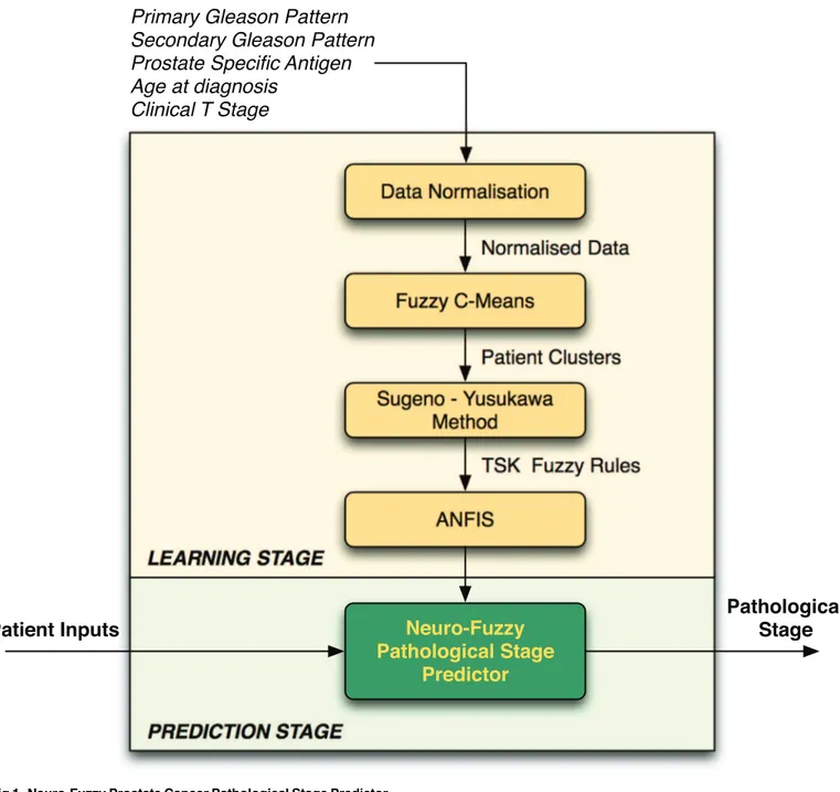
The neuro-fuzzy system proposed herein (a combination of fuzzy logic-based algorithms that are illustrated inFig 1) predicts the pathological stage of cancer (i.e. diagnosis outcome), using data that are obtained from pre-operative clinical tests that are conducted at the progno-sis stage. As with the TNM system, our proposed neuro-fuzzy system predicts whether a patient has organ-confined disease (OCD, pathological stage pT2) or extra-prostatic disease (ED, pathological stage>pT2).
Fig 1. Neuro-Fuzzy Prostate Cancer Pathological Stage Predictor.
The clinical data used for pathological cancer stage prediction are typically affected by imprecision, primarily due to the fact that not all patients exhibit abnormal results in all clinical tests. This poses a problem when trying to predict the progression of the cancer and therefore deciding on the best treatment strategy for patients. Hence, fuzzy logic is a suitable approach for this type of clinical prediction because it can be used to model human reasoning—in real scenarios the clinician would consider the data and give an estimation rather than a definite answer. The neuro-fuzzy system will make a prediction about a particular patient and return a value representing the‘degree of membership’of the patient’s cancer in the extra-prostatic set. The proposed framework is illustrated inFig 1and described in the subsections that follow.
The neuro-fuzzy model comprises two main stages: learning and prediction. At thelearning stage, the model trains itself using patient records for which the pathological stage is known, and at theprediction stagethe model predicts the pathological stage using the knowledge which has been obtained during the learning stage. The following subsections describe the processes that are involved during the learning and prediction stages.
System Inputs
At thelearning stage, the neuro-fuzzy predictor learns (i.e. trains itself) using existing patient record data in order to create the knowledge which will be used (during theprediction stage) to make predictions on new, and previously unseen, data. During the learning stage, the system takes as input data relating to each patient’s clinical features (i.e. age at diagnosis, PSA, biopsy Primary Gleason pattern, biopsy Secondary Gleason pattern, and clinical T stage) and known pathological stage results (i.e. known outputs) that have been obtained during diagnosis. The system represents the inputs as a matrixAof sizen×m, wherenis the total number of patient records, andmis the total number of clinical features (i.e. system inputs,m= 5). The system represents the targets in the form of an× 1 vector T, where each celltiholds the pathological T stage (pT) value for each patient record.
At theprediction stage, the system only requires as input an 1 ×mvector holding the results of a patient’s clinical features (i.e. age at diagnosis, PSA, biopsy Primary Gleason pattern, biopsy Secondary Gleason pattern, and clinical T stage), and the system will return a value rep-resenting the likelihood of the patient having Extra-Prostatic Disease (i.e. pathological stage results).
Data Normalisation
The age, PSA level, clinical T stage and pathological stage (pT) variables must be grouped before they are input into the fuzzy predictor. The normalisation of the values is described in theResultsSection. The normalisation process is performed in order to ensure a balanced dis-tribution among the data and to remove any outliers from the data which could affect the per-formance of the predictor algorithm.
Fuzzy C-Means
Formally, letA= [v1,v2,v3,. . .,vn] be the [patient record cases]-by-[clinical features] matrix and let 2c<nbe an integer, wherecis the number of clusters (i.e. classes) andnis the total number of patient record cases. In this particular prostate cancer application,c= 2 since we have two clusters: Organ-Confined Disease (OCD) and Extra-Prostatic Disease (ED). The Fuzzy C-Means (FCM) algorithm returns a list of cluster centersX=x1,. . .,xcand a member-ship matrixU=μi,k2[0, 1];i= 1,. . .,n;k= 1,. . .,c, where each elementμikholds the total
grades for each data point, representing a patient record, by iteratively moving the cluster cen-ters to the correct location within a data set. Essentially, this iteration process is based on mini-mizing an objective function which represents the distance from any given data point to a cluster center weighted by that data point’s membership grade. The objective function for FCM is a generalisation ofEq (1)
JðU;c1;. . .;c
cÞ ¼
Xc
i¼1
XN
k¼1
mmikjjvk xijj
2
;1m 1 ð1Þ
whereμikrepresents the degree of membership of patient recordviin theithcluster;xiis the
cluster centre of fuzzy groupi; |||| is the Euclidean distance betweenithcluster andjthdata point; andm2[1,1] is a weighting exponent. The necessary conditions forfunction (1)to reach its minimum are shown in functions (2) and (3).
ci ¼
PN k¼1m
m ikvk
PN
k¼1m m i;k
; ð2Þ
mik¼ 1
Pc
k¼1
jjvk xijj
jjvk xijj
2=ðm 1Þ
; ð3Þ
Sugeno-Yusukawa Method
A collection of Takagi-Sugeno-Kang (TSK) rules [23], one for each cluster, for determining the membership of a patient record to a particular cluster are generated. This Sugeno-type Fuzzy Inference System (FIS) is generated using the FCM clustering algorithm. The number of clus-ters derived from the clustering process determines the number of rules and membership func-tions in the generated FIS. The FIS structure maps inputs through input membership funcfunc-tions and associated parameters, and then through output membership functions and associated parameters to outputs. The output FIS is passed into the Adaptive-Neuro Fuzzy Inference Sys-tem (ANFIS) model [24] which then tunes the FIS parameters using the input/output training data in order to optimise the prediction model.
Adaptive-Neuro Fuzzy Inference System
with FCM, and thus the FIS returned from FCM clustering is input into the ANFIS, and the FIS parameters are tuned using the input/output training data in order to optimise the predic-tion model.
The training process stops whenever the designated epoch number is reached, or the error goal is achieved. The performance of ANFIS is evaluated using the array of root mean square errors (difference between the FIS output and the training data output) at each epoch. Thus, the membership degree of a patient record into a particular cluster (e.g. Extra-Prostatic Dis-ease), determines how close a prediction is to the next cluster (e.g. Organ-Confined Disease). In simple terms, letcaandcbbe cluster Extra-Prostatic Disease and cluster Organ-Confined Disease respectively, a patient recordvkcan belong to clustercasuch thatvk2ca, or it can belong in the intersection area between two clusters such thatvk2ca^vk2cb.
Neuro-Fuzzy Predictor
The neuro-fuzzy predictor takes as input a vectorXiof size 1 ×m, wheremis the total number of clinical features, hence 1 × 5 and the patient’s record is clustered as Organ-Confined Disease or Extra-Prostatic Disease, via the FCM clustering algorithm [26]. The predetermined Takagi-Sugeno-Kang (TSK) rules [23] are then applied in order to evaluate the degree of membership of the patient’s record to a particular cluster. The output is a numerical value representing the likelihood of a patient belonging to the Extra-Prostatic Disease cluster. This value is particu-larly useful when deciding on the suitable treatment to be offered to the patient. For example, treatment might be different if a patient is predicted as having Organ-Confined Disease with a value which leans more toward Extra-Prostatic Disease.
Methods II
—
Other Computational Intelligence Approaches
Artificial Neural Network Classifier
An Artificial Neural Network (ANN) can be trained to recognise patterns in data and this is a suitable approach for solving classification problems involving two or more classes. For the prostate cancer staging prediction problem, the ANN is trained to recognise the patients which have Organ-Confined Disease or Extra-Prostatic Disease. The pattern recognition neural net-work used was a two-layer feedforward netnet-work, in which the first layer has a connection from the network input and is connected to the output layer which produces the network’s output. Alog-sigmoid transfer functionwas embedded in the hidden layer, and asoftmax transfer func-tionwas embedded in the output layer.
of the weights and biases of the network in order to optimise network performance which is measured by the mean squared error network function.
Naive Bayes Classifier
Although the Naive Bayes classifier is designed for use when predictors within each class are independent of one another within each class, it is known to work well even when that inde-pendence assumption is not valid. The Naive Bayes classifies data in two steps. The first step is the training (i.e. learning) step which uses the training data, which are patient cases and their corresponding pathological cancer stage (i.e. Organ-Confined Disease or Extra-Prostatic Dis-ease), to estimate the parameters of a probability distribution, assuming predictors are condi-tionally independent given the class. The second step is the prediction step, during which the classifier predicts any unseen test data and computes the posterior probability of that sample belonging to each class. It subsequently classifies the test data according to the largest posterior probability. The following Naive Bayes description is based on that presented by Han et. al [8]. LetP(ci|X) be the posterior probability that a patient recordXiwill belong to a classci(class can be Organ-Confined Disease or Extra-Prostatic Disease), given the attributes of vectorXi. LetP(ci) be the prior probability that a patient’s record will fall in a given class regardless of the record’s characteristics; andP(X) is the prior probability of recordX, and hence the probability of the attribute values of each record. The Naive Bayes classifier predicts that a recordXi
belongs to the classcihaving thehighest posterior probability, conditioned onXiif and only if
P(ci|X)>P(cj|X) for 1jm,j6¼i, maximisingP(ci|X). The classcifor whichP(ci|X) is
maxi-mised is called themaximum posteriori hypothesisand estimated usingformula (4)
PðcijXÞ ¼
PðXjciÞPðciÞ
PðXÞ : ð4Þ
To predict the class label of a given recordXi,P(X|ci)P(ci) is evaluated for each classci. The classifier predicts that the class label of recordXiis the classciif and only if
PðXjciÞPðciÞ>PðXjcjÞPðcjÞ ð5Þ
for 1jm,j6¼i.
The Naive Bayes outcome is that each patient’s record, which is represented as a vectorXi, is mapped to exactly one classci, whereci= 1,. . .,nwherenis the total number of classes, i.e.
n= 2. The Naive Bayes classification function can be tuned on the basis of an assumption regarding the distribution of the data. Experiments were conducted using two methods of den-sity estimation: the first one assumes normality and models each conditional distribution with a single Gaussian; and the second uses nonparametric kernel density estimation. Hence, the Naive Bayes classifier was tuned using two functions: a Gaussian distribution (GD) and the Kernel Density Estimation (KDE). The Gaussian distribution assumes that the variables are conditionally independent given the class label and thereby exhibit a multivariate normal dis-tribution, whereaskernel density estimationdoes not assume a normal distribution and hence it is a non-parametric technique.
Support Vector Machine Classifier
generalisation error of the linear classifier is defined by the separating hyperplane. Support vec-tors are the points that reside on the canonical hyperplanes and are the elements of the training set that would change the position of the dividing hyper plane if removed. As with all super-vised learning models, a support vector machine is initially trained on existing data records, after which the trained machine is used to classify (predict) new data. Various Support Vector Machine kernel functions can be utilised to obtain satisfactory predictive accuracy.
The Support Vector Machine finds the Maximum Marginal Hyperplane (MMH) and the support vectors using a Lagrangian formulation and solving the equation using the Karush-Kuhn-Tucker (TTK) conditions, details of which can be found in [28]. Once the Support Vec-tor Machine has been trained, the classification of new unseen patient records is based on the Lagrangian formulation. For many‘real-world’practical problems, using the linear boundary to separate the classes may not reach an optimal separation of hyperplanes. However, Support Vector Machine kernel functions which are capable of performing linear and nonlinear hyper-plane separation exist. The outcome of applying the Support Vector Machine for prediction is that each patient record, represented as a vectorXi, is mapped to exactly one class labelyi, whereyi= ±1, such that (X1,y1), (X2,y2),. . .(Xm,ym), and henceyican take one of two values, either−1 or +1 corresponding to the classes Organ-Confined Disease and Extra-Prostatic
Dis-ease. Further details on the Support Vector Machine can be found in [29], and [30].
Results I: Dataset Analysis
Dataset Description
The Cancer Genome Atlas (TCGA) Research Network provides datasets for cancer patients which are made open to the public through the Data Coordinating Center and the TCGA Data Portal. The prostate cancer dataset obtained from the TCGA contains records collected from 399 patients diagnosed with a type ofProstate Adenocarcinoma Acinar, during the years 2000–
2013. All patients had prostate needle core biopsies for diagnosis before they underwent prosta-tectomy, and all patients had undergone a prostatectomy. The variables selected from the data-set were those that are used for performing prostate cancer stage predictions by clinicians, and which are also required for undertaking staging prediction using the AJCC pTNM Nomogram [21]—namely, biopsy Primary and Secondary Gleason patterns, pre-treatment PSA level, patient’s age at diagnosis, clinical T stage, and pathological T stage.
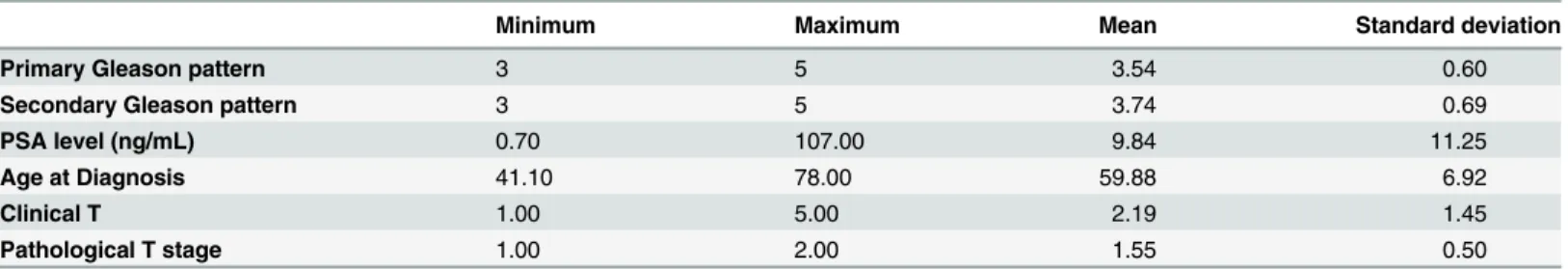
The age and PSA variables were categorically divided into groups that were chosen in order to ensure a balanced distribution between the data, as described later in this section.Table 4 provides statistics about the variables before they were categorised.
The Primary and Secondary Gleason pattern variables (seeTable 5) did not require any modification, as they are already categorically divided into three groups.
Table 4. Dataset Statistics.
Statistics of variables before categorisation
Minimum Maximum Mean Standard deviation
Primary Gleason pattern 3 5 3.54 0.60
Secondary Gleason pattern 3 5 3.74 0.69
PSA level (ng/mL) 0.70 107.00 9.84 11.25
Age at Diagnosis 41.10 78.00 59.88 6.92
Clinical T 1.00 5.00 2.19 1.45
Pathological T stage 1.00 2.00 1.55 0.50
The variables of pre-treatment total serum PSA levels and age were categorically divided into groups, as described in Tables6and7.Table 6shows how the PSA values have been grouped, the number of cases in each group (i.e. count), and their percentage. The histogram inFig 2illustrates the frequency distributions of the grouped PSA values.
Table 7displays how the age values have been grouped, the number of patient cases in each group (i.e. count), and the percentage of cases. Although it is very unlikely for a patient to have prostate cancer under the age of 35, there is still a possibility, and for this reason, groupings 1 to 4 have been formed. However, none of the patient cases fall in this category in the particular dataset which was used in the current study. This does not affect the performance of the system
Table 5. Primary and Secondary Gleason pattern groups.
Primary Gleason pattern groups Frequency count Proportion of patients(%)
3 205 51.4
4 173 43.4
5 21 5.3
Total 399 100.0
Secondary Gleason pattern groups Frequency count Proportion of patients(%)
3 159 39.8
4 185 46.4
5 55 13.8
Total 399 100.0
doi:10.1371/journal.pone.0155856.t005
Table 6. PSA groups.
PSA group PSA range Frequency count Proportion of patients (%)
1 0–2.5 ng/mL 16 4.01
2 2.6–4.0 ng/mL 33 8.27
3 4.1–6.0 ng/mL 124 31.08
4 6.1–9.9 ng/mL 124 31.08
5 10–19 ng/mL 67 16.79
6 20 ng/mL 35 8.77
doi:10.1371/journal.pone.0155856.t006
Table 7. Age groups.
Age group Age range Frequency count Proportion of patients (%)
1 <25 0 0
2 25–29 0 0
3 30–34 0 0
4 35–39 0 0
5 40–44 5 1.25
6 45–49 22 5.51
7 50–54 68 17.04
8 55–59 97 24.31
9 60–64 100 25.06
10 65–69 76 19.05
11 >70 31 7.77
in any way, and these groupings were included in order to create a comprehensive prediction system.
The clinical T and pathological T stage variable values were grouped as shown in Tables8 and9respectively. The clinical T stage variable values were grouped in such a way so as to match the groups that are presented on the TNM nomogram. Group 1 includes T stages T1a-c, which reflects the fact that tumor is present in one or both lobes by needle biopsy, but is not identifiable on the basis of palpation or is reliably visible by imaging. Group 2 includes clinical T stages in which the cancer is unilateral, meaning that it is located on one-half of one side or less; group 3 is unilateral and involves more than one-half of one side, but not both sides; group 4 is when the cancer is in the form of bilateral disease which is located on both sides of
PSA group
0 1 2 3 4 5 6
Frequency
0 20 40 60 80 100 120 140
Fig 2. Histogram of grouped PSA values.
doi:10.1371/journal.pone.0155856.g002
Table 8. Clinical T stage groups.
Clinical T group Clinical T stage Frequency count Proportion of patients (%)
1 T1(a-c) 204 51.13
2 T2a 53 13.28
3 T2b 53 13.28
4 T2c 42 10.53
5 T3a 29 7.27
5 T3b 16 4.01
5 T4 2 0.50
Total 399 100.00
the prostate; and group 5 is an Extra-Prostatic Disease, meaning that the cancer has started to spread (or has spread) to the bladder neck, rectum, and/or nearby organs.
The independent variable (i.e. predictor variable) of the dataset is the pathological T (pT) stage, whose values have been categorised as 1 for Organ-Confined Disease (OCD) and 2 for Extra-Prostatic Disease (ED). There is no pathologic pT1 classification, and pathological T stage values in the pT2 range indicate an Organ-Confined Disease and pathological T stage val-ues in the range of 3–4 indicate an Extra-Prostatic Disease.
Given that the aim of the model was to predict whether a patient has organ-confined disease (OCD, TNM pathological stagepT2) or extra-prostatic disease (ED, TNM pathological stage >pT2), and not the likelihood of cancer-related death (DOD, dead of disease), the pT3 and pT4 groupings were consolidated. T3a, T3b and T4 disease are all considered as being‘ high-risk disease’and strongly considered for active treatment, whereas those with lower categories of disease might instead be considered for active surveillance.Table 9includes the groupings of the pathological T stage values.
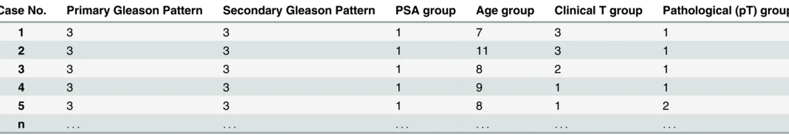
Tables10and11present a sample of the data before and after data normalisation (i.e. cate-gorically divided into groups), respectively. As previously mentioned, the values of Primary and Secondary Gleason patterns did not require any transformation, as they were already grouped.
Age at Diagnosis and its Association with PSA Values
Evidence indicates that age could be a contributing factor to increased PSA levels [16], and for this reason it is informative to investigate whether there are any associations between PSA lev-els and age in the dataset. The histograms illustrating the frequency distributions of the grouped PSA levels and age are illustrated in Figs2and3respectively. The meanage at diagno-sisof patients was 59.88 ± 6.92, and the meanpre-treatment PSA levelwas 9.84 ± 11.25. Table 12shows the mean and standard deviation PSA values of each age group.
Table 9. Pathological T (pT) stage groups.
pT group Pathological T (pT) stage Frequency count Proportion of patients (%) OCD or ED
1 T2(unknown if a or b) 1 0.25 OCD
1 T2a 14 3.51 OCD
1 T2b 47 11.78 OCD
1 T2c 117 29.32 OCD
2 T3a 142 35.59 ED
2 T3b 72 18.05 ED
2 T4 6 1.50 ED
Total 399 100.00
doi:10.1371/journal.pone.0155856.t009
Table 10. Before data normalisation.
Case No. Primary Gleason Pattern Secondary Gleason Pattern PSA Age Clinical T stage Pathological (pT) stage
1 3 3 1.00 51.6 T2b T2a
2 3 3 1.70 77.0 T2b T2c
3 3 3 2.05 55.2 T2a pT2b
4 3 3 2.09 61.1 T1c pT2b
5 3 3 2.20 57.0 T1c T3a
n . . . .
Table 11. After data normalisation.
Case No. Primary Gleason Pattern Secondary Gleason Pattern PSA group Age group Clinical T group Pathological (pT) group
1 3 3 1 7 3 1
2 3 3 1 11 3 1
3 3 3 1 8 2 1
4 3 3 1 9 1 1
5 3 3 1 8 1 2
n . . . .
doi:10.1371/journal.pone.0155856.t011
Age group
4 5 6 7 8 9 10 11
Frequency
0 10 20 30 40 50 60 70 80 90 100
Fig 3. Histogram of grouped age values.
doi:10.1371/journal.pone.0155856.g003
Table 12. PSA levels categorised by age group.
Age group Patient count PSA mean Standard deviation of PSA values
5 5 4.40 1.14
6 22 4.14 0.89
7 68 3.54 1.23
8 97 3.75 1.20
9 100 3.74 1.14
10 76 3.75 1.21
11 31 3.81 1.56
Total 399 3.75 1.21
To investigate if there is a statistically significant association between age and PSA levels, a Spearman’s rho correlation test was performed. The results revealed no significant associations among age and PSA levels (r= 0.003,p= 0.948), at least over the age ranges (40 to 78) that were included in the dataset which was used. A one-way ANOVA was also conducted to test for statistically significant differences between the PSA values of the various age groups. The test indicated that there were no statistically significant differences among any of the groups,
F(6,392) = 0.956,p= 0.455,p>0.05). Since age and PSA values are not associated, then both variables were used as inputs by the prediction system.
Analysis of the Clinical T Stage Values
The clinical T stage values are the results of a Digital Rectal Examination (DRE) test.Table 8 shows the total number of patients for each clinical T stage. As shown inTable 8, the clinical stage values of T1 (n= 204, 51.13%), T2a (n= 53, 13.28%), T2b (n= 53, 13.28%), T2c (n= 42, 10.53%), denote an Organ-Confined Disease cancer stage, and the T3a (n= 29, 7.27%), T3b (n= 16, 4.01%), T4 (n= 2, 0.50%) denote an Extra-Prostatic Disease cancer stage. At a clinical stage, a total of 352 patients (88.22%) exhibited Organ-Confined Disease, and a total of 47 patients exhibited Extra-Prostatic Disease (11.78%). Clearly, the results of the clinical T test alone is not as reliable as the pathological T (pT) test for determining the stage of prostate can-cer. This is evident since, at the pathological stage (i.e. diagnosis stage), out of the 399 patients, a total of 44.86% (n= 179) had Organ-Confined Disease, and 55.14% (n= 220) had Extra-Pros-tatic Disease, meaning that 43.36% (n = 173) patients with Extra-ProsExtra-Pros-tatic Disease were misdi-agnosed as having Organ-Confined Disease. DRE is not always a reliable test, since the location of the tumor within the prostate might influence the capacity to feel it.
Analysis of the Pathological T (pT) Stage Values
Table 9shows the total number of patients for each pathological T stage. As shown inTable 9, the pathological T stage values of T2a-c denote an Organ-Confined Disease cancer stage, and the pathological T stage values of T3a,b,T4 denote an Extra-Prostatic Disease cancer stage. Of the 399 patients, a total of 44.86% (n= 179) exhibited Organ-Confined Disease, and 55.14% (n = 220) exhibited Extra-Prostatic Disease.
Table 13shows the relationship between the prediction variables and prostate cancer with Organ-Confined Disease and Extra-Prostatic Disease. A one-way ANOVA test revealed signifi-cant differences between the means of the two groups for the biopsy Primary Gleason pattern (F(1,397) = 7.87,p= 0.005,p<0.05), biopsy Secondary Gleason pattern (F(1,397) = 5.83,
p= 0.016,p<0.05), and clinical T stage (F(1,397) = 5.062,p= 0.025,p<0.05) variables. These
Table 13. Mean and Standard deviation values for Organ-Confined Disease (OCD) and Extra-Prostatic Disease (ED) groups diagnosed at the Pathological stage.
Groups
Variables OCD ED p
n = 179 n = 220
Primary Gleason pattern 3.45±0.52 3.61±0.64 0.005 Secondary Gleason pattern 3.65±0.64 3.81±0.71 0.016
Pre-treatment PSA level (ng/mL) 3.76±1.26 3.74±1.17 0.848 Age at diagnosis (groups) 8.49±1.37 8.60±1.40 0.434 Clinical T stage 2.01±1.36 2.33±1.51 0.025
results were expected, since Gleason 1 grading of the biopsy determines the aggressiveness of the cancer, and hence patients with Extra-Prostatic Disease are more likely to have a higher value in this category than patients with Organ-Confined Disease. The same applies for PSA levels, as these tend to increase with progressive and more extensive disease. In addition, the clinical T stage values determine the outcome of a physical examination and the higher the number of the clinical T stage value, the more the disease has progressed. Interestingly, in this particular dataset, no statistically significant differences among the means values of the pre-treatment PSA levels (F(1,397) = 0.037,p= 0.848,p>0.05) and age (F(1,397) = 0.614,
p= 0.434,p>0.05) variables were apparent. Although the mean age of patients with Extra-Prostatic Disease was higher than that of patients with Organ-Confined Disease, this difference is not statistically significant. Also, there were no statistically significant differences among the mean PSA values of patients with Extra-Prostatic Disease and Organ-Confined Disease. In summary, the mean values of all but the PSA and age variables were significantly higher in the Extra-Prostatic Disease than in the Organ-Confined Disease groups.
Results II: Pathological Stage Prediction Using the Neuro-Fuzzy
Model
Experiment Methodology
Having analysed the dataset and, as appropriate, grouped the data, the next step is to explain how the transformed data will be input into the neuro-fuzzy model and the other models which will be used for the comparison process. In particular, the performance of the neuro-fuzzy model is compared to other computational intelligence based approaches, namely the Artificial Neural Network, Fuzzy C-Means, Support Vector Machine, and the Naive Bayes clas-sifier. All of these classifiers are suitable for solving prediction problems, as is the American Joint Committee on Cancer (AJCC) pTNM Nomogram [21] which is a statistical approach that is commonly adopted by clinicians for predicting prostate cancer staging. For predicting the pathological stage of cancer, the AJCC pTNM Nomogram uses all variables except the age at diagnosis variable. These variables are found inTable 13.
System Inputs
patients with Extra-Prostatic Disease fall in a higher range than the results of patients with Organ-Confined Disease.
The performance of the proposed neuro-fuzzy model was compared to that of an Artificial Neural Network, Fuzzy C-Means, Support Vector Machine, and the Naive Bayes classifiers; and the AJCC pTNM Nomogram statistical approach [21] which can also be considered as a classifier. The subsections below give a brief introduction to each classification model and details on how the parameters of each model were appropriately tuned in order to report their best performance.
3 3.5 4 4.5 5
0 0.5 1
Gleason 1
Degree of membership
OCD ED
3 3.5 4 4.5 5
0 0.5 1
Gleason 2
Degree of membership
OCD ED
1 2 3 4 5 6
0 0.5 1
PSA
Degree of membership
OCD ED
5 6 7 8 9 10 11
0 0.5 1
Age
Degree of membership
OCD ED
1 2 3 4 5
0 0.5 1
Clinical T stage
Degree of membership
OCD ED
Fig 4. Neuro-Fuzzy System Membership Functions: Gleason 1 is Primary Gleason Pattern; Gleason 2 is Secondary Gleason pattern; PSA is Prostate Specific Antigen; Age represents the Age group; and clinical T stage is the result of the Digital Rectal Examination.OCD is Organ-Confined Disease and ED is Extra-Prostatic Disease.
Performance Evaluation Measures
The evaluation measures that were adopted for assessing the performance of each approach for predicting the pathological stage of patients areSensitivityandSpecificity. These statistical mea-sures are used for evaluating the performance of binary classification tests and are suitable since the aim is to measure the performance of each system in distinguishing Extra-Prostatic Disease from the Organ-Confined Disease.
Sensitivity (i.e. True Positive Rate) measures the proportion of actual positives which are correctly identified as such (e.g. the percentage of Extra-Prostatic Disease patients who are cor-rectly identified as Extra-Prostatic Disease). Specificity (i.e. True Negative Rate) measures the proportion of negatives which are correctly identified as such (e.g. the percentage of patients with Organ-Confined Disease who are correctly identified as not having Extra-Prostatic Dis-ease). A perfect system would return 100% sensitivity (e.g., all patients with Extra-Prostatic Disease are classed as Extra-Prostatic Disease) and 100% specificity (e.g. all patients with Organ-Confined Disease are not classed as Extra-Prostatic Disease). The following notation relates to the evaluation measures.
• Let |TP| be the total number of patients with Extra-Prostatic Disease correctly classified as Extra-Prostatic Disease.
• Let |TN| be total the number of patients with Organ-Confined Disease correctly classified as Organ-Confined Disease.
• Let |FP| be the total number of patients with Organ-Confined Disease incorrectly classified as Extra-Prostatic Disease.
• Let |FN| be the total number of patients with Extra-Prostatic Disease incorrectly classified as Organ-Confined Disease.
• Let |P| be the total number of Extra-Prostatic Disease cases that exist in the dataset, where |P| = |TP| + |FN|.
• Let |N| be the total number of patients with Organ-Confined Disease that exist in the dataset, where |N| = |FP| + |TN|.
The functions for the Sensitivity and Specificity evaluation measures are presented in Func-tions (6) and (7) respectively.
SensitivityðkÞ ¼ jTPj
jTPj þ jFNj;2 ½0;1: ð6Þ
SpecificityðkÞ ¼ jTNj
jTNj þ jFPj;2 ½0;1: ð7Þ
The closer the values of Sensitivity and Specificity are to 1.0, the better the detection perfor-mance of the system.
and the low number of false positives. Maximizing sensitivity corresponds to some large True Positive Rate (y-axis value) on the ROC curve, and maximizing specificity corresponds to a small False Positive Rate value (x-axis value) on the ROC curve. Thus, the optimal cutoff value is to the upper left corner of the chart, the higher the overall accuracy of the classifier. Hence, a system which perfectly discriminates Organ-Confined Disease and Extra-Prostatic Disease has 1.0 (or 100%) sensitivity and 1.0 (or 100%) specificity.
Comparison of the Neuro-Fuzzy Model with Other Methods
The aim of the evaluation is to measure the ability of each system to predict the pathological stage of patients. The results presented in this section are those for validating the system, as these determine the true ability of a system to discriminate Organ-Confined Disease from Extra-Prostatic Disease using the knowledge which has been acquired by the system during the training (i.e. learning) process. To perform these evaluations, the actual outputs returned by each system during the validation stage were compared against the targets (i.e. known) outputs.
The results of the comparisons are shown inTable 14and illustrated inFig 5. The ROC curves for all systems are shown inFig 6. The cutoff points of each classifier are presented in
Table 14. Performance evaluation.
Performances based on ROC evaluation measurements
Neuro-Fuzzy (Our approach) FCM Quadratic-SVM ANN GB-NB AJCC pTNM Nomogram
Area Under the Curve (AUC) 0.812 0.809 0.738 0.699 0.750 0.582
Optimal ROC point FPR 0.274 0.403 0.242 0.303 0.274 0.032
Optimal ROC point TPR 0.789 0.901 0.718 0.701 0.775 0.197
Asymp. Sig. (McNemars) 1.000 0.868 0.499 1.000 1.000 0.000
doi:10.1371/journal.pone.0155856.t014
AUC False Positive ORP True Positive ORP 0
0.1 0.2 0.3 0.4 0.5 0.6 0.7 0.8 0.9 1
Our Approach FCM
Quadratic SVM ANN
GB−NB Nomogram
rows, Optimal ROC point False Positive Rate and Optimal ROC point True Positive Rate, of Table 14and were computed with the alpha values set toα= 0.05 (95% Confidence Interval).
The best system would return the largest AUC, a high number of true positives, and a low number of false positives.
The Support Vector Machine was trained using the Linear kernel function, Quadratic, Gaussian Radial Basis (GRB), Multilayer Perceptron kernel (MP) functions. The results of test-ing the performance (i.e. validation) of the Support Vector Machine ustest-ing the various kernel functions are presented inTable 15. The results show that the Quadratic-Support Vector Machine has the largest AUC (AUC= 0.738), thereby outperforming all other functions.
The Naive Bayes classifier results, when tuned using the Gaussian Distribution (i.e. normal distribution) and Kernel Density Estimation functions, are presented inTable 16. The results revealed that the Gaussian Naive Bayes (GD-NB) classifier returned a larger AUC
(AUC= 0.750), thereby outperforming the Kernel Density Estimation Naive Bayes (KDE-NB) classifier (AUC= 0.696).
0 0.1 0.2 0.3 0.4 0.5 0.6 0.7 0.8 0.9 1
0 0.1 0.2 0.3 0.4 0.5 0.6 0.7 0.8 0.9 1
False Positive Rate (1−Specificity)
True Positive Rate (Sensitivity)
Our Approach FCM
Quadratic SVM ANN
GD−NB Nomogram
Fig 6. ROC Curves: Performance Comparison.
doi:10.1371/journal.pone.0155856.g006
Table 15. Support Vector Machine(SVM) performance evaluation when applying various kernel functions.
Kernel Function
Evaluation Measure Linear Quadratic GRB MP
Specificity (TNR) 0.758 0.758 0.661 0.597
Sensitivity (TPR) 0.704 0.718 0.747 0.690
Area Under the Curve 0.731 0.738 0.704 0.644
Optimal ROC point FPR 0.242 0.242 0.339 0.403
Optimal ROC point TPR 0.704 0.718 0.747 0.690
The best Support Vector Machine and Naive Bayes classifiers are included inTable 14which contains all of the results. The results of the comparison revealed that the proposed neuro-fuzzy system, at its optimal point, returns the largest AUC, with a low number of false positives (FPR= 0.274,TPR= 0.789,AUC= 0.812). Although the FCM classifier returned the highest number of true positives, it returned a very high number of false positives (FPR= 0.403,
TPR= 0.901,AUC= 0.809). For these reasons, FCM cannot be considered as the optimum clas-sifier. The Quadratic-Support Vector Machine, ANN, and GB-NB did not perform as well as the neuro-fuzzy approach—they returned a smaller AUC, and a lower optimal TPR. The AJCC pTNM Nomogram performed the worst, with the smallest AUC (0.582), and the lowest number of TPR (0.197) at the optimal ROC point. The proposed neuro-fuzzy system therefore outper-formed all other systems.
Finally,Table 14shows the results of the McNemar test which was applied to investigate whether any statistically significant differences exist among each system’s target outputs and the actual outputs. The McNemar test is a statistical test which is applied on paired nominal data. It uses an approximate chi-square test of goodness to test the null hypothesis, i.e. there are no significant differences among targets and outputs. Each pair comprised of the actual and predicted values of each system. A good system will not return a statistically significant differ-ence (i.e.p>0.05) amongst its predicted outputs and the actual target outputs (known out-puts). The results revealed that there were no statistically significant differences among the actual and predicted outputs of the proposed neuro-fuzzy approach (p= 1.000,p>0.05); the FCM classifier, (p= 0.868,p>0.05); the Quadratic-SVM, (p= 0.499,p>0.05); the ANN (p= 1.000,p>0.05); and the GB-NB, (p= 1.000,p>0.05). However, there was a statistically significant difference among the outputs of the AJCC pTNM Nomogram against targets (p= 0.00,p<0.05).
Discussion and Conclusion
At the clinical prostate cancer staging process, the patient undergoes various clinical tests for the prognosis of prostate cancer, and based on these tests, the clinician estimates (or predicts) how much the cancer has spread. It is only after surgery, and hence at the pathological stage, that it is possible to more accurately diagnose cancer and determine the extent of its spread beyond the prostate gland. The ability to predict that pathological stage of prostate cancer is important, as it allows clinicians to determine the best approach for treating and managing the disease.
Herein, we propose the application of a neuro-fuzzy based approach for the prediction of the pathological stage of prostate cancer. The algorithm is suitable for the particular problem due to the imprecision, and the uncertainty which is typically found in the results of the clinical tests which can be used for predicting the pathological stage of prostate cancer. The system
Table 16. Naive Bayes(NB) performance evaluation using the Gaussian distribution and Kernel Den-sity Estimation functions.
Type of function
Evaluation Measure GD-NB KDE-NB
Specificity (TNR) 0.726 0.645
Sensitivity (TPR) 0.745 0.747
Area Under the Curve 0.750 0.696
Optimal ROC point FPR 0.274 0.355
Optimal ROC point TPR 0.775 0.747
input comprised of variables Primary and Secondary Gleason patterns, PSA levels, age at diag-nosis, and clinical T stage. The output is the pathological stage of the cancer which can be either Organ-Confined Disease or Extra-Prostatic Disease. Experiments were performed using an existing and validated prostate cancer patient dataset comprisingn= 399 patient records obtained from The Cancer Genome Atlas (TCGA) Research Network. The performance of the proposed neuro-fuzzy system was compared to other classifiers: the Artificial Neural Network, Fuzzy C-Means, Support Vector Machines, the Naive Bayes, and the AJCC pTNM Nomogram [21]. The results revealed that the proposed neuro-fuzzy system outperformed all other classifi-ers. Our results appear to be consistent to those of Castanho et al. [12] who have also developed genetic-fuzzy expert system for predicting whether prostate cancer if confined or not-confined. Their results have also revealed that computational intelligence approaches based on fuzzy algorithms are suitable for prostate cancer staging prediction, and exceed the performance of nomograms.
The algorithm proposed by Castanho et al. [12] tunes the membership functions using a genetic algorithm, whereas we have used the Adaptive Neuro Fuzzy Inference System (ANFIS) to optimise the membership functions. Furthermore, Castanho et al.’s [12] and our proposed system both aim to predict whether a patient has organ-confined disease (OCD, pathological stage pT2) or extra-prostatic disease (ED, pathological stage>pT2). Although both systems use pre-operative serum PSA, clinical stage, and primary and secondary Gleason grades of a biopsy to predict the pathological stage of prostate cancer, our system considers age as an additional input variable. Castanho et al.’s [12] genetic-fuzzy system achieved an Area Under the Curve of 0.824 which they compared against Partin probability tables which have been proposed by Makarov et al. [31], and which only achieved an Area Under the Curve of 0.693. Our proposed neuro-fuzzy approach achieved an Area under the curve of 0.812, and the AJCC nomogram achieved an Area Under the Curve of 0.582. These results approximate to those reported by Castanho et al. [12], and reveal a high degree of consistency among the two outcomes of the two studies, despite the fact that different datasets were used for each study. The nomograms used by Castanho et al., and the AJCC nomogram both use the TNM Classification of Malignant Tumors grading system [32]. A major limitation of the AJCC nomogram is that the biopsy Gleason 7 values are not split into 3 + 4 = 7 vs. 4 + 3 = 7 which have drastically different clinical outcomes. The proposed neuro-fuzzy model considers the Gleason Grades 3 + 4 and 4 + 3, and this was one of the reasons that it performed better than the AJCC nomogram.
A recent study by Tsao et al. [15] has also reported similar AUC values, to those returned by our model and that of Castanho et al. [12], when using the Partin probability tables proposed which have been proposed by Makarov et al. [31] to predict the pathological stage of prostate cancer in patients prior to receiving radical prostatectomy. Tsao et al. [15] developed an artifi-cial neural network (ANN) model to predict the pathological stage of prostate cancer and eval-uated the model on 299 patients, of whom 109 (36.45%) displayed prostate cancer with extra-capsular extension (ECE), and 190 (63.55%) displayed organ-confined disease (OCD). Overall, their results revealed that the ANN model (AUC= 0.795) significantly outperformed a Linear Regression statistical model (AUC= 0.746), and the Partin Tables (AUC= 0.695).
A study by Tamblyn et al. [36] which compared the Cancer of the Prostate Risk Assessment (CAPRA) score [37] against the Kattan (version 1998) [34] and Stephenson nomograms (ver-sion 2006) [38] revealed that the Kattan (version 1998) [34] tool was the best predictor of abso-lute risk of recurrence. Furthermore, a recent study by Boehm et al. [39] which compared three preoperative models, D’Amico [40], CAPRA [37] and Stephenson [38], revealed that these tools are reliable in North American patients, but have shortcomings for identifying patients at high risk of prostate cancer death in Europe. D’Amico [40] and CAPRA [37] include the amount of tumor detected on biopsy as part of their risk prediction algorithm and consider vol-ume to have an influence on the risk of disease recurrence. However, from the evidence pre-sented in Boehm et al. [39], this is not necessarily the case for non-US patients. Therefore, the precise influence of tumor volume on the risk of disease is inconclusive. Finally, although the volume of tumour per each core has been used to determine the significance of the tumor, Gleason 6 disease is still regarded as being a non-significant pathology, whereas Gleason 7 or greater is thought to be significant disease, irrespective of volume. As such, volume of disease adds very little to the decision-making process.
Currently, the proposed framework has been implemented as a research tool, and once more evaluations are conducted, the tool will be developed as a simple to use application which can be made accessible to clinicians. The tool will take the clinical test results (i.e. age at diagno-sis, PSA, biopsy Primary and Secondary Gleason patterns, and clinical T stage) of an individual patient and predict his likelihood of having extra-prostatic cancer, and thereby aid the clinical decision-making process. Ongoing work is applying the proposed neuro-fuzzy predictor to a larger dataset, examining other computational intelligence approaches, and continuing the development of novel algorithms for predicting disease status in patients with prostate cancer.
Author Contributions
Conceived and designed the experiments: GC AGP MK DB. Performed the experiments: GC. Analyzed the data: GC. Contributed reagents/materials/analysis tools: GC. Wrote the paper: GC DB GA RR MK AGP. Performed the data analysis: GC. Designed the prediction model: GC. Performed the experiments: GC. Drafted the manuscript: GC. Contributed equally with GC in writing and revising the entire manuscript and also in writing the clinical elements of the manuscript: AGP. Contributed significantly in writing the clinical elements of the manu-script and in revising the manumanu-script: MK RR. Contributed significantly to the design and experimental part of the study and in revising the manuscript: DB. Contributed to the design of the prediction model: GA. Participated in the preparation of the final manuscript: GC GA DB RR MK AGP. Read and approved the final manuscript: GC GA DB RR MK AGP.
References
1. Blute M, Nativ O, Zincke H, Farrow G, Therneau T, Lieber M. Pattern of failure after radical retropubic prostatectomy for clinically and pathologically localized adenocarcinoma of the prostate: influence of tumor deoxyribonucleic acid ploidy. J Urol. 1989; 142:1262–1265. PMID:2810503
2. Epstein J, Pizov G, Walsh P. Correlation of pathologic findings with progression after radical retropubic prostatectomy. Cancer. 1993; 71:3582–3593. doi:10.1002/1097-0142(19930601)71:11%3C3582::
AID-CNCR2820711120%3E3.0.CO;2-YPMID:7683970
3. Epstein J, Walsh P, Carmichael M, Brendler C. Pathologic and clinical findings to predict tumor extent of nonpalpable (stage T1c) prostate cancer. JAMA. 1994; 271:368–374. doi:10.1001/jama.1994.
03510290050036PMID:7506797
4. Dotan ZA, Ramon J. Nomograms as a tool in predicting prostate cancer prognosis. European Urology Supplements. 2009; 8(9):721–724. doi:10.1016/j.eursup.2009.06.013
5. Briganti A, Karakiewicz PI, Joniau S, Van Poppel H. The Motion: nomograms should become a routine tool in determining prostate cancer prognosis. European Urology. 2009; 55(3):743–747. doi:10.1016/j.
6. Chun FKH, Karakiewicz PI, Briganti A, Walz J, Kattan MW, Huland H, et al. A critical appraisal of logistic regression-based nomograms, artificial neural networks, classification and regression-tree models, look-up tables and risk-group stratification models for prostate cancer. BJU International. 2007; 99 (4):794–800. doi:10.1111/j.1464-410X.2006.06694.xPMID:17378842
7. Tewari A, Porter C, Peabody J, Crawford ED, Demers R, Johnson CC, et al. Predictive modeling tech-niques in prostate cancer. Molecular Urology. 2001; 5(4):147–152. doi:10.1089/10915360152745812 PMID:11790275
8. Han J. Data Mining: concepts and techniques. San Francisco, CA, USA: Morgan Kaufmann Publish-ers Inc.; 2005.
9. Benecchi L. Neuro-fuzzy system for prostate cancer diagnosis. Urology. 2006; 68(2):357–361. doi:10.
1016/j.urology.2006.03.003PMID:16904452
10. Keles A, Hasiloglu AS, Keles A, Aksoy Y. Neuro-fuzzy classification of prostate cancer using NEF-CLASS-J. Computers in Biology and Medicine. 2007; 37(11):1617–1628. doi:10.1016/j.compbiomed.
2007.03.006PMID:17531217
11. Çinar M, Mehmet E, Erkan ZE, Ateşçi ZY. Early prostate cancer diagnosis by using artificial neural
net-works and support vector machines. Expert Syst Appl. 2009; 36(3):6357–6361. doi:10.1016/j.eswa. 2008.08.010
12. Castanho MJP, Hernandes F, De RèAM, Rautenberg S, Billis A. Fuzzy expert system for predicting pathological stage of prostate cancer. Expert Systems with Applications. 2013; 40(2):466–470. doi:10. 1016/j.eswa.2012.07.046
13. Saritas I, Ozkan IA, Sert IU. Prognosis of prostate cancer by artificial neural networks. Expert Systems with Applications. 2010; 37(9):6646–6650. doi:10.1016/j.eswa.2010.03.056
14. Shariat SF, Kattan MW, Vickers AJ, Karakiewicz PI, Scardino PT. Critical review of prostate cancer pre-dictive tools. Future Oncol. 2009; 5(10):1555–84. doi:10.2217/fon.09.121PMID:20001796
15. Tsao CW, Liu CY, Cha TL, Wu ST, Sun GH, Yu DS, et al. Artificial neural network for predicting patho-logical stage of clinically localized prostate cancer in a Taiwanese population. Journal of the Chinese Medical Association. 2014; 77(10):513–518. doi:10.1016/j.jcma.2014.06.014PMID:25175002
16. Burford D, Kirby M, Austoker J. Prostate cancer risk management programme: information for primary care PSA testing in asymptomatic men. NHS Cancer Screening Programmes; 2009.
17. Schröder FH, Hugosson J, Carlsson S, Tammela T, Määttänen L, Auvinen A, et al. Screening for pros-tate cancer decreases the risk of developing metastatic disease: findings from the European Random-ized Study of Screening for Prostate Cancer (ERSPC). European Urology. 2012; 62(5):745–752. doi:
10.1016/j.eururo.2012.05.068PMID:22704366
18. Luján M, PáezÀ, Berenguer A, Rodríguez JA. Mortality due to prostate cancer in the Spanish arm of the European Randomized Study of Screening for Prostate Cancer (ERSPC). Results after a 15-year follow-up. Actas Urológicas Españolas (English Edition). 2012; 36(7):403–409.
19. Heijnsdijk E, Wever E, de Koning H. Cost-effectiveness of prostate cancer screening based on the European Randomised Study of Screening Pprostate Cancer. The Journal of Urology. 2012; 187(4, Supplement):e491. doi:10.1016/j.juro.2012.02.1502
20. Falzarano SM, Magi-Galluzzi C. Staging prostate cancer and its relationship to prognosis. Diagnostic Histopathology. 2010; 16(9):432–438. doi:10.1016/j.mpdhp.2010.06.010
21. Edge S, Byrd DR, Compton CC, Fritz AG, Greene FL, Trotti A. AJCC Cancer Staging Manual. 7th ed. New York, NY: Springer; 2010.
22. Zadeh LA. Fuzzy sets. Information and Control. 1965; 8(3):338–353. doi:10.1016/S0019-9958(65) 90241-X
23. Sugeno M, Yasukawa T. A fuzzy-logic-based approach to qualitative modeling. IEEE Transactions on Fuzzy Systems. 1993; 1(1):7–31. doi:10.1109/TFUZZ.1993.390281
24. Jang JSR. ANFIS: adaptive-network-based fuzzy inference system. Systems, Man and Cybernetics, IEEE Transactions on. 2002; 23(3):665–685. doi:10.1109/21.256541
25. Jang JSR. Input selection for ANFIS learning. In: Proceedings of the IEEE International Conference on Fuzzy Systems; 1996. p. 1493–1499.
26. Bezdek JC. Pattern recognition with fuzzy objective function algorithms. Norwell, MA, USA: Kluwer Academic Publishers; 1981.
27. Möller MF. A scaled conjugate gradient algorithm for fast supervised learning. Neural Networks. 1993; 6(4):525–533. doi:10.1016/S0893-6080(05)80056-5
29. Cristianini N, Shawe-Taylor J. An introduction to support vector machines and other kernel-based learning methods. New York, NY, USA: Cambridge University Press; 2000.
30. Hastie T, Tibshirani R, Friedman J. The elements of statistical learning. Springer Series in Statistics. New York, NY, USA: Springer New York Inc.; 2001.
31. Makarov DV, Trock BJ, Humphreys EB, Mangold LA, Walsh PC, Epstein JI, et al. Update nomogram to predict pathologic stage of prostate cancer given prostate-specific antigen level, clinical stage, and biopsy Gleason score (Partin Tables) based on cases from 2000 to 2005. Urology. 2007; 6(69):1095– 1101. doi:10.1016/j.urology.2007.03.042
32. Sobin L, Wittekind C. TNM classification of malignant tumors. 5th ed. John Wiley and Sons, Inc., New York; 1997.
33. Brawer K, Cuzick J, Cooperberg M, Swanson G, Freedland S, Reid J, et al. Prolaris: a novel genetic test for prostate cancer prognosis. Journal of Clinical Oncology. 2013; 31.
34. Kattan M, Eastham J, Stapleton A, Wheeler T, Scardino P. A preoperative nomogram for disease recur-rence following radical prostatectomy for prostate cancer. Journal of the National Cancer Institute. 1998; 10(90):766–71. doi:10.1093/jnci/90.10.766
35. Partin AW, Mangold LA, Lamm DM, Walsh PC, Epstein JI, Pearson JD. Contemporary update of pros-tate cancer staging nomograms (Partin Tables) for the new millennium. Urology. 2001; 58(6):843–848.
doi:10.1016/S0090-4295(01)01441-8PMID:11744442
36. Tamblyn D, Chopra S, Yu C, Kattan M, Pinnock C, Kopsaftis T. Comparative analysis of three risk assessment tools in Australian patients with prostate cancer. Journal of the British Association of Uro-logical Surgeons. 2011; 108(2):51–66.
37. Cooperberg M, Pasta D, Elkin E, Litwin M, Latini D, Du CJ, et al. The University of California, San Fran-cisco Cancer of the Prostate Risk Assessment score: a straightforward and reliable preoperative pre-dictor of disease recurrence after radical prostatectomy. The Journal of Urololgy. 2005; 173(6):1938– 42. doi:10.1097/01.ju.0000158155.33890.e7
38. Stephenson AJ, Scardino PT, Eastham JA, Bianco FJ, Dotan ZA, Fearn PA, et al. Preoperative Nomo-gram Predicting the 10-Year Probability of Prostate Cancer Recurrence After Radical Prostatectomy. Journal of the National Cancer Institute. 2006; 98:715–717. doi:10.1093/jnci/djj190PMID:16705126
39. Boehm K, Larcher A, Beyer B, Tian Z, Tilki D, Steuber T, et al. Identifying the Most Informative Predic-tion Tool for Cancer-specific Mortality After Radical Prostatectomy: Comparative Analysis of Three Commonly Used Preoperative Prediction Models. European Urology. 2015;.
![Table 1. Definitions of clinical TNM according AJCC 2010 [21].](https://thumb-eu.123doks.com/thumbv2/123dok_br/17152814.240209/5.918.308.867.552.1051/table-definitions-clinical-tnm-according-ajcc.webp)
![Table 3. Anatomic stage/prognostic groups (from AJCC 2010) [21].](https://thumb-eu.123doks.com/thumbv2/123dok_br/17152814.240209/6.918.56.865.737.1048/table-anatomic-stage-prognostic-groups-ajcc.webp)