www.atmos-chem-phys.net/16/1511/2016/ doi:10.5194/acp-16-1511-2016
© Author(s) 2016. CC Attribution 3.0 License.
Origin of oxidized mercury in the summertime free troposphere
over the southeastern US
V. Shah1, L. Jaeglé1, L. E. Gratz2, J. L. Ambrose3,a, D. A. Jaffe1,3, N. E. Selin4, S. Song4, T. L. Campos5, F. M. Flocke5, M. Reeves5, D. Stechman5, M. Stell5, J. Festa6, J. Stutz6, A. J. Weinheimer7, D. J. Knapp7, D. D. Montzka7,
G. S. Tyndall7, E. C. Apel7, R. S. Hornbrook7, A. J. Hills7, D. D. Riemer8, N. J. Blake9, C. A. Cantrell10, and R. L. Mauldin III10,11
1Department of Atmospheric Sciences, University of Washington, Seattle, WA, USA 2Environmental Program, Colorado College, Colorado Springs, CO, USA
3School of Science, Technology, Engineering and Mathematics, University of Washington-Bothell, Bothell, WA, USA 4Department of Earth, Atmospheric and Planetary Sciences, Massachusetts Institute of Technology, Cambridge, MA, USA 5Earth Observing Laboratory, National Center for Atmospheric Research, Boulder, CO, USA
6Department of Atmospheric and Oceanic Sciences, University of California, Los Angeles, CA, USA 7Atmospheric Chemistry Observations and Modeling Laboratory, National Center for Atmospheric Research,
Boulder, CO, USA
8Rosenstiel School of Marine and Atmospheric Science, University of Miami, Miami, FL, USA 9Department of Chemistry, University of California, Irvine, CA, USA
10Department of Atmospheric and Oceanic Sciences, University of Colorado, Boulder, CO, USA 11Department of Physics, University of Helsinki, Helsinki, Finland
anow at: College of Engineering and Physical Sciences, University of New Hampshire, Durham, NH, USA Correspondence to:V. Shah ([email protected])
Received: 17 August 2015 – Published in Atmos. Chem. Phys. Discuss.: 5 October 2015 Revised: 12 January 2016 – Accepted: 15 January 2016 – Published: 10 February 2016
Abstract. We collected mercury observations as part of the Nitrogen, Oxidants, Mercury, and Aerosol Distributions, Sources, and Sinks (NOMADSS) aircraft campaign over the southeastern US between 1 June and 15 July 2013. We use the GEOS-Chem chemical transport model to in-terpret these observations and place new constraints on bromine radical initiated mercury oxidation chemistry in the free troposphere. We find that the model reproduces the observed mean concentration of total atmospheric mer-cury (THg) (observations: 1.49±0.16 ng m−3, model: 1.51±
0.08 ng m−3), as well as the vertical profile of THg. The
ma-jority (65 %) of observations of oxidized mercury (Hg(II)) were below the instrument’s detection limit (detection limit per flight: 58–228 pg m−3), consistent with model-calculated
Hg(II) concentrations of 0–196 pg m−3. However, for
ob-servations above the detection limit we find that modeled Hg(II) concentrations are a factor of 3 too low (observa-tions: 212±112 pg m−3, model: 67±44 pg m−3). The
high-est Hg(II) concentrations, 300–680 pg m−3, were observed in
or-der to maintain the modeled global burden of THg, we need to increase the in-cloud reduction of Hg(II), thus leading to faster chemical cycling between Hg(0) and Hg(II). Observa-tions and model results for the NOMADSS campaign sug-gest that the subtropical anticyclones are significant global sources of Hg(II).
1 Introduction
Exposure to mercury affects the human nervous system, hin-ders cognitive development in children, and causes cardio-vascular diseases in adults (Mergler et al., 2007; Karagas et al., 2012). In fish, mammals, and birds, mercury can ad-versely affect reproductive behavior (Scheuhammer et al., 2007). Although mercury is naturally present in our envi-ronment, human activities have increased its concentrations in the atmosphere and ocean by factors of 3 to 7 (Lamborg et al., 2002; Selin, 2009; Strode et al., 2010; Amos et al., 2013; Zhang et al., 2014) making mercury exposure a major public health concern.
In the troposphere, 90 % of mercury occurs in its elemen-tal form (Hg(0)) in the gas phase, while the rest is in the oxi-dized (mercuric, +2) state (Hg(II)), either in the gas-phase or bound to particles (Gustin et al., 2013). The chemical forms of atmospheric Hg(II) have not been identified, but laboratory and theoretical studies suggest that they likely in-clude HgCl2, HgBr2, HgBrBrO, HgBrNO2, HgBrHO2, HgO, HgSO4, Hg(NO3)2, and Hg(OH)2(Gustin et al., 2013;
Dib-ble et al., 2012; Huang et al., 2015). Both natural and anthro-pogenic processes emit mercury to the atmosphere, mostly as Hg(0). Atmospheric Hg(II) originates predominantly from the oxidation of Hg(0), with a minor contribution from di-rect anthropogenic emissions (Driscoll et al., 2013). Un-like Hg(0), Hg(II) is highly water-soluble and reactive, and is quickly scavenged from the atmosphere by rainwater or aerosol particles, such that 60 % of the global mercury de-position is estimated to occur by wet and dry dede-position of Hg(II) (Selin et al., 2008; Holmes et al., 2010).
Atomic bromine (Br) has been observed as the main oxi-dant of atmospheric Hg(0) in the polar and the marine bound-ary layers (Lindberg et al., 2002; Ebinghaus et al., 2002; Lau-rier et al., 2003; Obrist et al., 2011), and laboratory studies (Ariya et al., 2002; Donohoue et al., 2006), theoretical calcu-lations (Goodsite et al., 2004, 2012; Balabanov et al., 2005; Dibble et al., 2012; Shepler et al., 2007), and modeling stud-ies (Holmes et al., 2006, 2010) suggest a predominant role of Br in the oxidation of Hg(0) in the global atmosphere. While other oxidants have been proposed, in particular OH and O3(Hall, 1995; Spicer et al., 2002; Pal and Ariya, 2004a,
b; Sumner et al., 2005; Rutter et al., 2012), theoretical studies (Calvert and Lindberg, 2005; Goodsite et al., 2004; Hynes et al., 2009) suggest that the bimolecular reaction of Hg(0) with O3and OH is too slow in the atmosphere, and the fast
rates observed in the laboratory could have been influenced
by wall-mediated reactions or formation of aerosol particles (Tossell, 2006; Subir et al., 2011).
Measurements at a few high-elevation sites have shown episodic enhancements of Hg(II) concentrations (350– 600 pg m−3) usually in low relative humidity and low CO air, suggesting efficient in situ production of Hg(II) in the free troposphere (Landis et al., 2005; Swartzendruber et al., 2006; Faïn et al., 2009; Sheu et al., 2010; Weiss-Penzias et al., 2015). Sillman et al. (2007) reported higher (60– 248 pg m−3) Hg(II) concentrations at 3 km altitude than near
the surface in aircraft flights off the Florida coast. Swartzen-druber et al. (2009) found a large variability in Hg(II) con-centrations (0–500 pg m−3) during five flights over the
Pa-cific Northwest below 5 km altitude, with higher trations in free-tropospheric air with low aerosol concen-trations. Lyman and Jaffe (2012) found enhanced Hg(II) concentrations of∼450 pg m−3 and depleted total mercury
(THg, THg = Hg(0)+Hg(II)) concentrations (<1 ng m−3) in
a stratospheric intrusion, suggesting rapid oxidation of Hg(0) and loss of Hg(II) above the tropopause. During multiple year-round flights over Tennessee, USA, Brooks et al. (2014) found that Hg(II) concentrations at 2–4 km altitude were 10– 30 times higher than those near the surface throughout the year. Typically, these past aircraft campaigns have focused on Hg(II) measurements over small spatial scales. The sparse-ness of free-tropospheric measurements of Hg(II) has hin-dered the validation of redox chemistry in global models of tropospheric mercury, which display large inter-model vari-ability in wet and dry deposition (Bullock et al., 2008, 2009; Travnikov et al., 2010).
The Nitrogen, Oxidants, Mercury, and Aerosol Distribu-tions, Sources, and Sinks (NOMADSS) aircraft campaign was conducted over the southeastern US to determine the distribution of THg and Hg(II) at a regional scale. Here, we analyze these observations using the GEOS-Chem chemical transport model with the goals of examining the origin of Hg(II) in the free troposphere and testing the kinetics of the Br-initiated oxidation mechanism.
2 Observations and model used in this study 2.1 The NOMADSS campaign
Figure 1.Flight tracks of the NSF/NCAR C-130 aircraft during the 19 NOMADSS research flights between 1 June and 15 July 2013. The flight tracks of four flights discussed in the text are highlighted (RF-06: green, RF-09: red, RF-10: brown, and RF-16: blue).
the University of Washington’s Detector of Oxidized Mer-cury Species (UW-DOHGS), which is currently the only in-strument capable of making simultaneous measurements of total and elemental mercury concentrations aboard an air-craft platform at a relatively high time resolution of 2.5 min (Swartzendruber et al., 2009; Lyman and Jaffe, 2012; Am-brose et al., 2013, 2015). In addition, the C-130 aircraft was equipped with other instruments summarized in Table 1.
This paper complements several other papers focused on the analysis of mercury measurements during NOMADSS. In particular, Gratz et al. (2015a) present an analysis of the high Hg(II) concentrations and BrO concentrations ob-served on one NOMADSS flight (research flight 6). Am-brose et al. (2015) use the NOMADSS observations to cal-culate enhancement ratios of Hg in the plumes of six coal-fired power plants, and compare them to the Hg emission ratios reported in the emission inventories. Song et al. (2014) combine the NOMADSS observations with results from the GEOS-Chem model to constrain Hg emissions from land and ocean sources. Gratz et al. (2015b) use the NOMADSS ob-servations over Lake Michigan and a plume dispersion model to quantify the outflow of Hg from the Chicago/Gary indus-trial area.
2.2 The UW-DOHGS instrument
The UW-DOHGS is a dual channel instrument that simul-taneously measures concentrations of THg and Hg(0). Am-brose et al. (2015) discuss the configuration of the instru-ment during NOMADSS, in-flight calibration as well as pre-and post-campaign laboratory tests. Briefly, the UW-DOHGS draws a fast flow of ambient air from a rear-facing aircraft in-let heated to 110◦C to facilitate transmission of Hg(II) com-pounds. Two Tekran® 2537B Hg vapor analyzers
subsam-ple the inlet flow at 1 L min−1 (at 0◦C and 1 atm) through parallel channels. The Tekran® analyzers sample Hg(0) by
Au-amalgamation pre-concentration on paired sample car-tridges, with quantification by cold vapor atomic fluores-cence spectrometry (CVAFS). The sample integration time and measurement time resolution are both 2.5 min. In the THg channel, Hg(II) compounds are reduced to Hg(0) by passing the sampled air through a quartz pyrolyzer heated to 650◦C. In the Hg(0) channel, Hg(II) (in gas and particle-bound phases) is removed using either a quartz wool trap (first fourteen flights) or a cation exchange membrane (re-maining five flights). Hg(II) concentrations are calculated from the difference between the THg and Hg(0) measure-ments. In comparison, the Tekran®2537-1130-1135 specia-tion system uses KCl denuders to capture gas-phase oxidized mercury, which is subsequently thermally desorbed as ele-mental mercury for analysis (Landis et al., 2002). The mea-surement cycle of the Tekran®speciation system is 30 min or longer, compared to the 2.5 min cycle for the UW-DOHGS. The UW-DOHGS is not affected by O3-interference, unlike
the Tekran® system (Lyman et al., 2010; Ambrose et al., 2013; McClure et al., 2014). A limitation of UW-DOHGS is that the quartz wool traps can release Hg(II) in humid con-ditions (Ambrose et al., 2013, 2015), which decreased the number of Hg(II) observations in the boundary layer during the first 14 flights. This was not a problem on the later five flights when cation exchange membranes were used in place of quartz wool.
During NOMADSS, the 1σ uncertainty in THg and Hg(0) was 8–10 %, and the detection limit (DL) was < 0.05 ng m−3. For Hg(II), the 1σ uncertainty varied between
38 pg m−3(at THg of 1.2 ng m−3) and 55 pg m−3(at THg of
2.8 ng m−3). The Hg(II) DL is calculated using the “same
air” configuration, in which the Hg(II) filter is bypassed and both analyzers sample the same air downstream of the py-rolyzer in the THg channel (Ambrose et al., 2013, 2015). The 3σ Hg(II) DL for the campaign ranged between 58 and 228 pg m−3.
The UW-DOHGS instrument was operational during all 19 flights of the NOMADSS campaign, and concentrations of THg were measured continuously during each flight, ex-cept during calibration cycles. A total of 2381 (2.5 min av-erage) observations of THg were made during the campaign. Hg(II) concentrations could be determined for only∼60 % of the time (1503 observations), because of periodic in-flight calibration cycles and because of reduced retention efficiency of the Hg(II) traps during some flight segments in the moist boundary layer. For the entire NOMADSS campaign, 35 % of the Hg(II) measurements (528 points out of 1503) were above the instrument’s DL. Here and in the rest of the paper, we use ADL (Above Detection Limit) observations to refer to Hg(II) measurements above the instrument’s DL and BDL (Below Detection Limit) for Hg(II) measurements below the DL. In the boundary layer (defined here as altitude<2 km and water vapor>8 g kg−1), 87 % of the 532 observations
Table 1.Chemical and meteorological measurements used in this work.
Observations Measurement technique Instrument model/Reference
THg, Hg(0), and Hg(II) Dual-channel CVAFS (UW-DOHGS) Lyman and Jaffe (2012); Ambrose et al. (2013, 2015) BrO Differential Optical Absorption Spectroscopy Platt and Stutz (2008) RH Chilled mirror hygrometry Buck 1011C CO Vacuum-UV Resonance Fluorescence Aero-Laser AL5001 NO, NO2, O3 NO2chemiluminescence Ridley et al. (2004) CH2O, CHBr3, C3H8 Gas chromatography/mass spectrometry Apel et al. (2010)
SO2 Pulsed fluorescence Thermo Scientific Model 43i-TLE
As more than half the Hg(II) observations during NOMADSS were BDL, we follow the recommendation of Helsel (2011) and use the robust regression on order statis-tics (ROS) method to assign values for BDL observations. The ROS method assumes a lognormal distribution for the observations, and estimates the distribution’s parameters us-ing ADL measurements. The BDL values are then estimated using the fitted distribution. The ROS method is applied to calculate Hg(II) means and standard deviations reported in Tables 3 and 4 and Figs. 2–5.
2.3 The GEOS-Chem model 2.3.1 General description
The GEOS-Chem global 3-D atmospheric chemical trans-port model (www.geos-chem.org) is driven by meteorologi-cal fields from the NASA Global Modeling and Assimilation Office (GMAO) Goddard Earth Observing System (GEOS) Version 5 Forward Processing (FP). The GEOS-5 FP sys-tem consists of a general circulation model (GCM) coupled with a data assimilation (DAS) system (Rienecker et al., 2008), with a native horizontal resolution of 0.25◦ latitude by 0.3125◦longitude and 72 vertical levels up to 0.01 hPa. The GEOS-5 FP meteorological fields are archived either at 1 or 3 h intervals, depending on the variables.
GEOS-Chem includes advection (Lin and Rood, 1996), convective transport (Wu et al., 2007), turbulent mixing (Lin and McElroy, 2010), wet deposition (Liu et al., 2001; Wang et al., 2011; Amos et al., 2012), and dry deposition (Wang et al., 1998; Zhang et al., 2011) of chemical species. The full-chemistry simulation includes an up-to-date chemical mech-anism for gas-phase and heterogeneous reactions of HOx -NOx-VOC-O3-aerosols in the troposphere (Bey et al., 2001)
with the recent addition of bromine chemistry (Parrella et al., 2012). We use here GEOS-Chem model version 9-02.
The GEOS-Chem Hg model simulates the emissions, chemistry, transport, and deposition of Hg(0) and Hg(II) in the atmosphere (Selin et al., 2007) with updates from Holmes et al. (2010), Amos et al. (2012), and Zhang et al. (2012), coupled with a 2-D ocean model (Strode et al., 2007; So-erensen et al., 2010) and a 2-D land model (Selin et al., 2008;
Holmes et al., 2010). The model includes prescribed emis-sions from biomass burning and geogenic activity (Holmes et al., 2010). The global GEOS-Chem Hg simulation, with a resolution of 4◦ latitude×5◦ longitude, was evaluated by Holmes et al. (2010), who found the modeled THg (1.71±0.5 ng m−3) to be in good agreement with
observa-tions (1.86±1.0 ng m−3, correlation coefficient=0.9) at 39
land-based sites across the globe. Simulated THg concentra-tions were about 10 % higher than THg concentraconcentra-tions mea-sured during three aircraft campaigns (INTEX-B, CARIBIC, and ARCTAS), but modeled vertical profiles were consis-tent with observations in the troposphere. Zhang et al. (2012) developed a nested-grid Hg simulation in GEOS-Chem, us-ing a higher horizontal resolution (0.5◦×0.667◦) over North America. They found that the average annual modeled wet deposition (7.2±3.2 µg m−2yr−1) at 95 Mercury Deposi-tion Network (MDN; http://nadp.sws.uiuc.edu/mdn/) sites was close to the observations (8.8±3.6 µg m−2yr−1) and showed a correlation coefficient of 0.78. The modeled an-nual mean THg concentrations (1.42±0.11 ng m−3) were
un-biased with respect to the observations (1.46±0.11 ng m−3)
at 19 surface-based sites. While the modeled gaseous Hg(II) concentrations at these sites were higher than the observa-tions by a factor of 1.5, the model captured the observed seasonal cycle with higher concentrations during spring and summer at most sites.
2.3.2 Updates to Hg emissions in GEOS-Chem
We have updated the global anthropogenic Hg emissions to the United Nations Environment Programme (UNEP)/Arctic Monitoring and Assessment Program (AMAP) 2010 (http:// www.amap.no/mercury-emissions/datasets), and over North America we use the U.S. EPA National Emissions Inventory (NEI) 2011 (http://www.epa.gov/ttnchie1/net/2011inventory. html) and Environment Canada’s National Pollutant Re-lease Inventory (NPRI) 2011 emission inventories. The spe-ciation of anthropogenic emissions is assumed to be 90 % Hg(0) : 10 % Hg(II) from all anthropogenic sources based on Zhang et al. (2012) and Kos et al. (2013). For 2013, the GEOS-Chem global emission of mercury is 1850 Mg a−1
sources and re-emission, and 225 Mg a−1 from biomass
burning. For 1 June–15 July 2013, the anthropogenic, nat-ural, and biomass burning emissions over North America are 130, 870, and 22 kg d−1, respectively.
2.3.3 Updates to Hg chemistry in GEOS-Chem
The oxidation of Hg(0) is modeled as a two-step reaction initiated by Br radicals as originally implemented in GEOS-Chem by Holmes et al. (2010), based on the work of Good-site et al. (2004); Donohoue et al. (2006), and Balabanov et al. (2005):
Hg(0)+Br−→M HgBr (R1)
HgBr+M→Hg(0)+Br+M (R2)
HgBr+Br→Hg(0)+Br2 (R3)
HgBr+X→Hg(II) (X=OH,Br,HO2,NO2,BrO)
(R4) We use the recently corrected rate constant for the HgBr dis-sociation Reaction (R2) (Goodsite et al., 2012). Holmes et al. (2010) had assumed Br and OH as the second-step oxidants (Reaction R4). In addition, based on the recommendations of Dibble et al. (2012), we have updated this mechanism to in-clude HO2, NO2, and BrO as the second-step oxidants. The
rates constants used here are
k1=1.46×10⁻³²×
T
298
−1.86
× [M]cm−3molecule−1s−1
(Donohoue et al., 2006) (1)
k2=2.67×1041exp
−7292 T
T 298
1.76
×k1s−1
(Goodsite et al., 2012) (2)
k3=3.9×10⁻¹¹cm−3molecule−1s−1
(Balabanov et al., 2005) (3)
k4=2.5×10⁻¹⁰×
T 298
−0.57
cm−3molecule−1s−1 (Goodsite et al., 2012; Dibble et al., 2012) (4) The reduction of Hg(II) to Hg(0) is assumed to occur in cloud droplets in the presence of sunlight. The reduction is assumed to be proportional to the photolysis frequency of NO2, and
the coefficient is estimated by constraining the model results with the observed mean burden of THg in the troposphere (Holmes et al., 2010). The uptake of Hg(II) by sea-salt parti-cles is simulated as a kinetic mass transfer process (Holmes et al., 2010). For non sea-salt aerosol particles, gas-particle partitioning is simulated as an equilibrium process based on an empirical relationship (Amos et al., 2012). The modeled wet and dry deposition of gas-phase Hg(II) is analogous to that of HNO3, and of particle-bound Hg(II) to that of sulfate
particles.
2.3.4 Simulations conducted for this study
In this study, the GEOS-Chem Hg model is run in a one-way nested-grid configuration, with the native horizontal resolu-tion (0.25◦×0.3125◦) over North America, and a coarser resolution (2◦×2.5◦) globally. Both the coarse- and fine-grid models share the same vertical resolution with 47 layers (13 layers in the bottom 2 km, and 16 layers between 2 and 10 km). The global Hg model is spun-up with a 3-year sim-ulation, and is then used to generate the initial and boundary conditions for the nested-domain, and to calculate the an-nual global mercury budget. Monthly concentrations of Br, BrO, OH, HO2, NO2, O3, and aerosols are obtained from
a 1-year 4◦×5◦global HOx–NOx–VOC–O3–BrOx-aerosols tropospheric chemistry GEOS-Chem simulation. We run the nested 0.25◦×0.3125◦ Hg model for North America from 1 June to 15 July 2013. For comparison to the NOMADSS aircraft observations, the model is sampled along the flight track at the 2.5 min time step of the UW-DOHGS instrument. In addition to the BASE simulation with the Hg(0)+Br chemistry described above (Sect. 2.3.3), we perform five sen-sitivity simulations (Table 2), and focus on two of them. In the first sensitivity simulation (3×Br) we increase the GEOS-Chem Br and BrO concentrations by a factor of 3 in the 45◦S to 45◦N latitude band between 750 hPa and the tropopause. Parrella et al. (2012) found that the GEOS-Chem BrO is within the BrO measurement uncertainties of the GOME-2 satellite in the polar regions and at mid-latitudes, but in the tropics the GEOS-Chem BrO is too low by a factor of 2–4 throughout the year (Fig. 5 of Parrella et al., 2012). Furthermore, recent aircraft-based observations of BrO in the tropical and subtropical free troposphere of the Southern Hemisphere reported concentrations which were 2–4 times higher than predicted by the GEOS-Chem model (Wang et al., 2015).
In the second sensitivity simulation (FastK), we replace the Donohoue et al. (2006) rate constant for Reaction (R1) by the faster rate constant measured by Ariya et al. (2002). Following Dibble et al. (2012), we proportionally increase the rate constant for the backward Reaction (R2) as follows:
k1,FastK=3.6×10⁻¹² ×
[M]T ,p [M]273.15 K,1 atm
cm−3molecule−1s−1 (Ariya et al., 2002)
k2,FastK=k2×
k1,FastK
k1
s−1
(Goodsite et al., 2012, Dibble et al., 2012). (5) Relative to the BASE simulation,k1,FastK and k2,FastK are
Table 2.Summary of GEOS-Chem simulations performed for this study.
Simulation Oxidants Reaction rate constants (cm3molecule−1s−1)
Main simulations
BASE Br (Concentrations from the GEOS-Chem Hg(0)+Br:k=1.46×10−32×298T −1.86
× [M]
full-chemistry simulation) (Donohoue et al., 2006) 3×Br Br (Concentrations scaled by a factor of 3
in the region bounded by 45◦S and 45◦N, Same as BASE and 750 hPa and the tropopause.)
FastK Same as BASE Hg(0)+Br:k=3.6×10⁻¹²×M MT ,p
273.15K,1atm
(Ariya et al., 2002)
Supplemental simulations
FastK+0.9BrO Same as FastK, except BrO concentrations in the free
troposphere over the northwest Atlantic Ocean Same as FastK were increased to 0.9 pptv only for RF-16 simulation.
BASE+OH/O3 Br, OH and O3(Concentrations from the Hg(0)+Br: same as BASE
GEOS-Chem full chemistry simulation) Hg(0)+O3:k=3.0×10⁻²⁰
(Hall, 1995)
Hg(0)+OH:k=8.7×10⁻¹⁴ (Sommar et al., 2001) BASE+BrO Br and BrO (Concentrations from the Hg(0)+Br: same as BASE
GEOS-Chem full chemistry simulation) Hg(0)+BrO:k=3.0×10⁻¹⁴
(Spicer et al., 2002)
BASE simulation. This enables us to isolate the model’s sen-sitivity to the redox chemistry of Hg.
At the 39 global land-based sites considered previously by Holmes et al. (2010), the results of the BASE (1.71 ng m−3),
3×Br (1.74 ng m−3), and FastK (1.64 ng m−3) models are
comparable to the observations (1.86 ng m−3). Figure S1 (in
the Supplement) shows a comparison with observations of the inter-hemispheric gradient and the seasonal cycle of total gaseous Hg concentrations.
3 Observed horizontal and vertical distribution of THg and Hg(II)
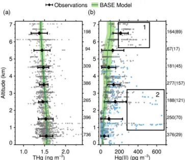
The vertical and horizontal distributions of THg and Hg(II) concentrations observed during NOMADSS are presented in Figs. 2 and 3. We exclude from these figures and the rest of our analysis fresh pollution plumes, where NOx, SO2, or C3H8 exceed 2 ppbv. This eliminates 6 % of the
THg and 4 % of the Hg(II) measurements. The mean and standard deviation of the observed THg concentrations was 1.49±0.16 ng m−3 (Fig. 3a). THg concentrations decrease slightly with altitude, from 1.54 ng m−3 near the surface to 1.38 ng m−3 at 6–7 km altitude (Fig. 2a), which is in agree-ment with previous aircraft-based measureagree-ments of THg over North America (Talbot et al., 2007; Swartzendruber et al., 2009; Mao et al., 2010). The variability in THg concentration is small, with standard deviations at different levels ranging
from 6 to 15 % of the mean concentrations. The weak vertical gradient and the low standard deviation of the THg concen-trations are consistent with the long tropospheric lifetime of THg.
For Hg(II), the observed mean concentration was 212±
112 pg m−3, for ADL measurements (35 % of measurements)
(Table 3). When we include BDL values using the ROS method (see Sect. 2.2), the mean Hg(II) concentration is 110±103 pg m−3 (Table 3). In order to assess the overall
mean distribution of Hg(II) during NOMADSS, Figs. 2b and 3c display the Hg(II) statistics that include BDL values esti-mated with the ROS method. Figure 2b shows that observed Hg(II) concentrations increased from 40 pg m−3 at 0–1 km altitude to 200 pg m−3at 6–7 km (Fig. 2b). Large enhance-ments in Hg(II) concentrations, of up to 500 pg m−3, were
observed at 5–7 km during two research flights (RF) over Texas (RF-06 and RF-09, box 1 in Figs. 2b and 3d). Concen-trations of up to 680 pg m−3were observed at 1–3 km on one
flight over the Atlantic Ocean (RF-16). We will discuss these flights in more detail in Sect. 6. Table S1 in the Supplement presents a summary of Hg(II) observations on all flights.
Table 3.Chemical characteristics of NOMADSS observations classified in four air mass categories.
All observations low RH/low CO low RH/high CO high RH/low CO high RH/high CO
No of THg observationsa 2381 233 551 212 1385
THg observations (ng m−3) 1.49±0.16 1.35±0.15 1.48±0.11 1.44±0.20 1.53±0.15 No of Hg(II) observationsb 1503 184 414 159 746
(ADL) (528) (132) (244) (47) (105)
Hg(II) all observations (pg m−3)c 110±103 239±141 146±81 108±123 48±57 (ADL)d (212±112) (289±136) (189±76) (249±140) (155±73) Altitude (km) 2.6±1.9 4.6±1.8 3.9±1.2 2.9±2.2 1.7±1.5
RH (%) 49±27 16±10 15±9 68±17 66±13
CO (ppbv) 107±33 65±4 97±13 65±3 124±30 O3(ppbv) 55±14 52±16 63±17 43±16 54±10 NOx(pptv) 158±156 55±32 67±34 44±39 232±170 CH2O (ppbv) 1.8±1.4 0.5±0.3 0.7±0.3 0.9±0.4 2.7±1.3 The four air mass categories are based on thresholds of RH=35%and CO=75ppbv. The mean and standard deviation for each category are indicated.aNumber of 2.5minTHg samples.bTotal number of 2.5minHg(II) samples, including samples below the detection limit (BDL). The number in parenthesis indicates the number of 2.5minHg(II) samples above the detection limit (ADL).cMean Hg(II) concentration and standard deviation for all observations, including BDL as estimated using the ROS method.dMean Hg(II) concentration and standard deviation for ADL observations.
Figure 2. Vertical profiles of (a) THg and (b) Hg(II) during NOMADSS. Individual 2.5 min observations are shown with grey circles (for THg and Hg(II) measured using the quartz wool filter) and blue squares (for Hg(II) measured using the cation exchange membrane filter). Observations above the detection limit (ADL) are indicated as filled circles/squares, while observations below the de-tection limit (BDL) are shown as open circles/squares and are es-timated using the regression on order statistics (ROS) method. The means and standard deviations calculated for 1 km vertical bins are shown for the observations (black diamonds and error bars) and the BASE GEOS-Chem simulation (green line and shading). The num-bers on the right hand side of each panel indicate the number of 2.5 min observations in each 1 km bin. For Hg(II), the second num-ber in parenthesis indicates the numnum-ber of ADL observations. The areas marked as “1” and “2” highlight measurements of high Hg(II) concentrations and are referenced in the text and Fig. 3.
based on the measured relative humidity (RH) and CO concentrations (Table 3). We use thresholds of RH=35 % and CO=75 ppbv to classify the observations into four categories: “high RH/high CO”, “high RH/low CO”, “low RH/high CO”, and “low RH/low CO”. When RH or CO mea-surements were not available (18 % of the observations), we use the GEOS-Chem simulated RH values and CO concen-trations. The ROS procedure is used to assign values for BDL observations separately for each category.
Using this method, Hg(II) observations partition into the four categories as follows (Table 3): “low RH/low CO” (12 % of observations), “low RH/high CO” (28 %), “high RH/low CO” (10 %), “high RH/high CO” (50 %). The highest mean concentrations of Hg(II) are found in the “low RH/low CO” category (239 pg m−3 for all observations, 289 pg m−3 for
ADL observations). Observations in this category had the lowest average THg concentrations (1.35 ng m−3), and were
relatively clean with low mixing ratios for CH2O (0.5 ppbv),
NOx(55 pptv), O3(52 ppbv), and a mean RH of 16 %. These
air samples were observed mainly during the high-altitude (5–7 km) flights over Texas (RF-06 and RF-09), and at 1– 3 km over the Atlantic on RF-16. The chemical characteris-tics and HYbrid Single-Particle Lagrangian Integrated Tra-jectory (HYSPLIT) (Draxler and Hess, 1998) back trajecto-ries for these “low RH/low CO” air masses indicate subsi-dence from the clean subtropical upper troposphere (Sect. 6). The “low RH/high CO” category displays moderate enhancements in Hg(II) concentrations, with a mean of 146 pg m−3(189 pg m−3for ADL observations). Back
trajec-tories (not shown here) indicate transport from high latitudes (>60◦N) accompanied by subsidence. The mean concentra-tions of NOx (67 pptv) and CH2O (0.7 ppbv) were low and
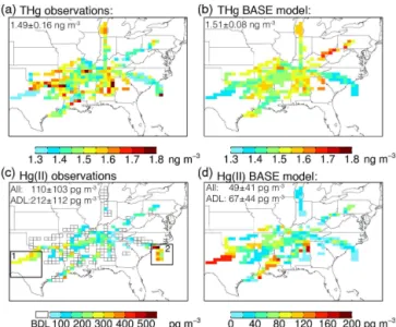
Figure 3.Horizontal distribution of THg (top panels) and Hg(II) (bottom panels). Observations are shown on panels(a, c), while re-sults from the BASE GEOS-Chem simulation are on panels(b, d). Observed and simulated values are averaged in 0.5◦ latitude by 0.625◦longitude columns. For Hg(II) observations, the means in-clude ROS estimates for values below the detection limit (BDL). Locations where all observed Hg(II) concentrations were BDL are shown by open squares. Note the different color scales for the ob-served and modeled Hg(II) concentrations(c, d). Regions marked as “1” and “2” highlight the areas with high Hg(II) and are refer-enced in the text and in Fig. 2. The numbers at the top of each panel indicate the means and standard deviations for all the modeled and observed concentrations. For Hg(II) we separate the statistics for all the measurements (“All”) and for the measurements above the detection limit (“ADL”).
mid- and upper-troposphere at high latitudes instead of trop-ical latitudes as in the “low RH/low CO” category.
Most of the remaining Hg(II) observations (50 % of ob-servations) fall in the “high RH/high CO” category. These observations were collected mainly in the continental bound-ary layer, with moderately high concentrations of CO (124 ppbv), CH2O (2.7 ppbv), and NOx (232 pptv). In this category, the mean concentration of THg is 1.53 ng m−3,
while that of Hg(II) is 48 pg m−3(155 pg m−3for ADL
ob-servations, which account for only 14 % of observations in this category). The “high RH/low CO” category has lower CO (68 ppbv), CH2O (0.9 ppbv), NOx (44 pptv), and O3
(43 ppbv). These samples were observed mostly near the ma-rine boundary layer over the Atlantic Ocean (14 and RF-16), but some were observed at high altitudes possibly in air detrained from clouds. In this category, the mean concentra-tion of THg is 1.44 ng m−3, and that of Hg(II) is 108 pg m−3 (249 pg m−3 for ADL observations, 30 % of the observa-tions).
The observations of Hg(II) during NOMADSS are simi-lar to previous observations of Hg(II) in terms of their mag-nitude, vertical profiles, and airmass characteristics. During
five summertime flights in the Pacific Northwest, Swartzen-druber et al. (2009) also found RGM (gaseous component of Hg(II)) to be generally below the instrument’s DL of 80–160 pg m−3. They found high RGM air masses (200– 500 pg m−3) on two flights at 2–6 km altitude. These air masses had low aerosol extinction coefficient, indicating ei-ther larger production of RGM at higher altitudes or loss of RGM in the presence of aerosol particles (Swartzen-druber et al., 2009). On 28 flights from August 2012 to June 2013, Brooks et al. (2014) found that mean RGM and PBM (particle-bound component of Hg(II)) concentrations at 0–6 km over Tennessee, USA were 34 and 30 pg m−3,
re-spectively. Highest concentrations on each flight were al-ways observed at 2–4.5 km altitude. RGM concentrations exhibited a minimum in the winter months and a maxi-mum in the summer months. On one flight in June 2013, the vertical profile of RGM showed a steep increase from the surface (∼5 pg m−3) to 4 km altitude (120 pg m−3)
fol-lowed by decrease between 4 and 6 km (70 pg m−3) (Brooks et al., 2014). At the high elevation Mt. Bachelor Observatory (2.7 km a.s.l.) in Oregon, the mean RGM concentration dur-ing May–August 2005 was 43 pg m−3(Swartzendruber et al.,
2006). Low RGM concentrations (<50 pg m−3) were seen in
boundary layer air during the day, and higher concentrations were seen in free-tropospheric air during the night. The high-est 10 % of nighttime RGM concentrations were between 160 and 600 pg m−3, and were measured in air with low RH and
low CO, in similarity to the observations of high Hg(II) in our “low RH/low CO” category during NOMADSS.
4 Comparison to the BASE GEOS-Chem Hg simulation
THg concentrations simulated in the BASE GEOS-Chem model (1.51±0.08 ng m−3) agree well with observations (1.49±0.16 ng m−3) (Fig. 3a, b). The model captures the lower THg concentrations observed over central Texas, South Carolina, and part of the Atlantic Ocean, but overes-timates THg concentrations over the Ohio River Valley by
∼20 %, possibly because of recent reductions in power plant emissions of mercury not captured in the 2011 NEI inven-tory used in our study. The model reproduces the vertical profile of observed THg, decreasing from 1.57 ng m−3
(ob-served: 1.54±0.15 ng m−3) near the surface to 1.43 ng m−3
(observed: 1.38±0.19 ng m−3) at 6–7 km altitude. However,
Table 4.Modeled THg and Hg(II) concentrations in the three GEOS-Chem Hg simulations for the four air mass categories.
All observations “low RH/low CO” “low RH/high CO” “high RH/low CO” “high RH/high CO”
Observed Hg(II) (pg m−3)
All 110±103 239±141 146±81 108±123 48±57 (ADL) 212±112 289±136 189±76 249±140 155±73
BASE model Hg(II) (pg m−3)
All 49±41 99±48 76±36 20±25 28±19 (ADL)a 67±44 96±51 75±34 14±18 38±19 (BDL)b 39±44 105±37 78±39 22±27 26±18
3×Br model Hg(II) (pg m−3)
All 62±72 162±104 91±67 28±41 29±28 (ADL)a 98±94 176±116 94±76 19±30 44±29 (BDL)b 43±94 124±47 86±51 31±45 26±27
FastK model Hg(II) (pg m−3)
All 80±98 208±144 128±95 18±25 34±32 (ADL)a 125±120 216±160 128±89 16±17 55±42 (BDL)b 55±120 189±88 129±102 19±28 31±28
Observed THg (ng m−3)
All 1.49±0.16 1.35±0.15 1.48±0.11 1.44±0.20 1.53±0.15 BASE model THg (ng m−3)
All 1.51±0.08 1.43±0.06 1.50±0.05 1.40±0.03 1.55±0.07 3×Br model THg (ng m−3)
All 1.51±0.11 1.40±0.09 1.50±0.08 1.36±0.04 1.55±0.10 FastK model THg (ng m−3)
All 1.52±0.09 1.44±0.07 1.52±0.06 1.40±0.04 1.55±0.08
aModel values corresponding to ADL observations.bModel values corresponding to BDL observations.
Because the majority of Hg(II) measurements are below the 58–228 pg m−3DL of the UW-DOHGS instrument, we
consider ADL and BDL observations separately. Table 4 shows that when observed Hg(II) are BDL (65 % of mea-surements), the mean Hg(II) concentrations predicted with the BASE simulation (39±34 pg m−3) are indeed below the
instrument’s DL. For ADL observations, the BASE model underestimates observations by a factor of 3 (model: 67±
44 pg m−3, observations: 212±112 pg m−3). The model
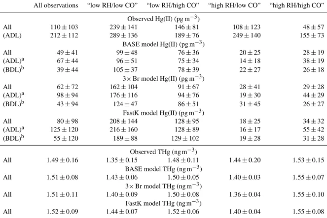
pre-dicts an increase in Hg(II) concentrations with altitude which is much smaller than observed (Fig. 2b). While underestimat-ing the observed mean concentrations, the model captures the factor of 3–6 increase in Hg(II) in the “low RH” air mass cat-egories relative to the “high RH” catcat-egories (Tables 3 and 4). Figure 5 shows scatter plots between observed and mod-eled Hg(II) concentrations for the “low RH/low CO” and “low RH/high CO” categories. We find that the GEOS-Chem BASE simulation has a large negative (−47 to−58 %) nor-malized mean bias (NMB=P
i(Mi−Oi) /PiOi), where Oi and Mi are observed and simulated values, and for Oi<DL,P
iOiis calculated using the ROS procedure). Fur-thermore, about 60 % of modeled Hg(II) values are within a factor of two of the observations (FAC2=fraction of points where 0.5≤Mi/Oi≤2, for Oi ≤DL, we assume 0.5≤
Mi/Oi≤2 ifMi<2×DL). If we consider only ADL ob-servations, FAC2 decreases to 28–39 %.
Figure S2 (in the Supplement) displays scatterplots for the “high RH” categories. For ADL observations, the NMB is between−75 and−94 % for these categories (Fig. S2 and Table 4). We note that for these two “high RH” categories a conclusive evaluation of the model performance is difficult, however, because of the large fraction of BDL observations. Considering the systematic model underestimate of ob-served Hg(II) concentrations, particularly in dry air masses where reduction and wet deposition are suppressed, we hy-pothesize that the bias in the Hg(II) concentrations is because the model simulated oxidation of Hg(0) to Hg(II) is too slow. We test this hypothesis in the next section by examining two sensitivity simulations.
Figure 4. Mean vertical profiles of(a)THg and(b) Hg(II) con-centrations averaged in 1 km vertical bins during NOMADSS. Ob-servations are shown with black diamonds (error bars indicate the standard deviation). BDL Hg(II) observations are estimated using the ROS method for each vertical bin. The means and standard devi-ations for the three model simuldevi-ations are shown as lines and shad-ing: BASE (green), 3×Br (blue), and FastK (orange).
simulations reproduce the observed mean concentration (Ta-ble 4) and vertical profile (Fig. 4a) of THg as we compensate the increase in Hg(0) oxidation with an increase in Hg(II) reduction rate to maintain the THg burden.
The 3×Br and FastK simulations predict a stronger ver-tical gradient in Hg(II) concentrations, in closer agreement with observations (Fig. 4). Above 5 km, Hg(II) concentra-tions in the 3×Br (165±104 pg m−3) and FastK (184±
156 pg m−3) simulations show significantly better agreement
with observations (189±103 pg m−3) relative to the BASE simulation (97±46 pg m−3) (Fig. 4b). For the “low RH/low CO” category, average modeled Hg(II) concentrations in-crease from 99±48 pg m−3 (BASE) to 162±104 pg m−3
(3×Br) and 208±144 pg m−3(FastK), compared to the
ob-served 239±141 pg m−3. The modeled NMB for all Hg(II)
observations in the “low RH/low CO” category decreases from −58 % (BASE simulation) to −32 % (3×Br) and
−12 % (FastK), while the FAC2 index increases from 62 % (BASE) to 69 % (3×Br) and 80 % (FastK) (Fig. 5a–c). How-ever, the sensitivity simulations cannot reproduce the high Hg(II) concentrations observed on RF-16 at 1–3 km (blue cir-cles in Fig. 5). We present a detailed discussion of this flight in Sect. 6.
In the “low RH/high CO” category, the 3×Br Hg(II) concentrations (91±67 pg m−3) are∼20 % higher than the BASE model (76±36 pg m−3), but lower than the observed concentrations (146±81 pg m−3) (Table 4). In the FastK sim-ulation, Hg(II) concentrations increase to 128±95 pg m−3,
improving the NMB (FastK:−11 %, 3×Br:−37 %, BASE:
−47 %) (Fig. 5d–f). For this category, the 3×Br Hg(II) con-centrations are not much higher than the BASE simulation
Figure 5.Scatterplot of observed and simulated concentrations of Hg(II) for the three model simulations in the(a–c)“low RH/low CO”, and(d–f)“low RH/high CO” categories. Each column corre-sponds to our three GEOS-Chem simulations: BASE (left column), 3×Br (middle column) and FastK (right column). Observations for RF-06 (green), RF-09 (orange), and RF-16 (blue) are highlighted in color, with the remaining observations indicated by gray symbols. The black circles and error bars represent the mean and standard de-viations of values below the detection limit (BDL) estimated with the ROS method for each air mass category separately and the cor-responding simulated concentrations. The Normalized Mean Bias (NMB) and fraction of points where the model is within a factor of 2 of the observations (FAC2) are indicated on each panel (see text for definitions).
because in the 3×Br we use higher Br concentration only between 45◦N and 45◦S, whereas most of the “low RH/high CO” air masses originated from high latitudes. The FAC2 in-dex is higher in the FastK simulation (75 %) compared to the BASE (58 %) and 3×Br (61 %) simulations.
Overall, the factor of 2 decrease in model bias for Hg(II) with the sensitivity simulations particularly for the “low RH/low CO” air samples suggests that the oxidation of Hg(0) in the upper troposphere is 3 (3×Br) to 5 (FastK) times faster than what was considered previously in the GEOS-Chem model.
We ran two additional simulations that included oxidation by OH/O3and by BrO, respectively, in addition to the
Hg(0)+O3→Hg(II) (R5)
Hg(0)+OH→Hg(II) (R6)
Hg(0)+BrO→Hg(II), (R7)
where k5=3.0×10⁻²⁰cm3molecule−1s−1 (Hall, 1995),
k6=8.7×10⁻¹⁴cm3molecule−1s−1(Sommar et al., 2001),
and k7=3.0×10⁻¹⁴cm3molecule−1s−1 (Spicer et al.,
2002).
The inclusion of Hg(0)+O3 and Hg(0)+OH pathways
decreases the global tropospheric chemical lifetime of Hg(0) for June–July 2013 from 3.2 months (BASE simulation) to 0.6 months, which is also lower than the lifetimes in the 3×Br (1.9 months) and the FastK (0.7 months) simulations. However, the Hg(0)+O3 and Hg(0)+OH reaction
path-ways have a relatively small effect on the modeled Hg(II) concentrations in the upper troposphere. The 5–7 km Hg(II) concentrations in this simulation (108±79 pg m−3) are
sim-ilar to the BASE simulation (97±45 pg m−3), but the Hg(II)
concentrations below 5 km (71±51 pg m−3) are higher than
the BASE simulation (39±33 pg m−3). The increase in
ox-idation with the Hg(0)+O3 and Hg(0)+OH pathways is
mostly in the lower troposphere, whereas in the upper tropo-sphere, faster oxidation is compensated by faster reduction. While the oxidation rates of Hg(0)+O3and Hg(0)+OH
re-actions have large uncertainties (see Sect. 1), our results in-dicate that the underestimate in Hg(II) concentrations in the BASE model persists despite the inclusion of the Hg(0)+O3
and Hg(0)+OH oxidation pathways.
When the Hg(0)+BrO oxidation pathway is added, the June–July global tropospheric chemical lifetime of Hg(0) is 0.9 months. The simulated 5–7 km Hg(II) concentrations (115±75 pg m−3) are higher than those in the BASE
simula-tion, but not as high as the 3×Br and FastK simulations, and much lower than the observations. The NMB for the “low RH/low CO” air masses is−47 % for this simulation, com-pared to−32 % for the 3×Br simulation and−12 % for the FastK simulation. Thus, although including the Hg(0)+BrO reaction with the rate from Spicer et al. (2002) brings the model closer to the observations, it does not completely ex-plain the model underestimate of Hg(II) concentrations.
6 Case studies of individual flights
We analyze in more detail three NOMADSS flights during which high concentrations of Hg(II) were observed. For RF-06 and RF-09 over Texas, we trace the origin of the high Hg(II) to transport from the subtropical Pacific anticyclone, while for RF-16 off the South Carolina Coast, enhanced Hg(II) concentrations appear to have been produced in the subtropical Atlantic anticyclone. The time series of the ob-servations and model results along the flight tracks are shown in Figs. 6–8.
6.1 RF-06 (19 June 2013) and RF-09 (24 June 2013) One of the goals of RF-06 was to sample in dry air masses with potentially enhanced Hg(II) concentrations. The me-teorological forecasts indicated the presence of such an air mass at 6 km altitude over west Texas. After sampling in the boundary layer, the aircraft ascended to 6.8 km altitude, measuring 182–347 pg m−3 of Hg(II) between 18:02 and
19:47 UTC (Fig. 6a and d). The Hg(II) DL on this flight was 114 pg m−3, and quartz wool was used as the Hg(II) filter
on the instrument’s Hg(0) channel. The mean concentration of THg in this air mass was 1.35 ng m−3, about 20 % lower
than the THg concentrations measured during the rest of the flight (Fig. 6b). The observed low RH (11 %), CO (65 ppbv), O3 (39 ppbv), NOx (53 pptv), CH2O (204 pptv), and C3H8
(36 pptv) indicate a clean and dry air mass (Fig. 6d). The 7-day HYSPLIT back trajectories (Fig. 6e) indicate that the air mass was transported from the subtropical Pacific anti-cyclone 3 days before it was sampled over Texas (see also Gratz et al., 2015a). The back trajectories show subsidence of the air mass from the upper troposphere (10–12 km) be-fore transport out of the Pacific anticyclone.
Figure 6c shows that the 3×Br simulation captures the enhancement in Hg(II) concentrations observed over Texas (observations: 251 pg m−3, 3×Br: 306 pg m−3), while the
BASE model (146 pg m−3) is too low and the FastK model
(367 pg m−3) too high. Outside the region with the high
Hg(II) concentration, all three model simulations calculate Hg(II) concentrations that are BDL, and are in agreement with the observations. During this flight, observations indi-cate high BrO concentrations of 1.9±0.35 pptv (Fig. 6d) (Gratz et al., 2015a). The GEOS-Chem modeled BrO con-centrations in this air mass (0.3–0.4 pptv) are a factor of 5 lower than the observations (Fig. 6d), and thus our assump-tion of higher Br concentraassump-tions in the 3×Br simulation is more consistent with these measurements (Sect. 2.3.4).
The transport pattern of dry air from the subtropical Pa-cific upper troposphere to the southeastern US persisted for several days and was sampled again on 24 June 2013 during flight RF-09 (Fig. 7a). High Hg(II) concentrations of 200– 480 pg m−3were measured between 16:00 and 19:30 UTC as
the C-130 aircraft flew five constant-altitude legs between 2.5 and 6.7 km over eastern Texas. The Hg(II) DL on this flight was 94 pg m−3, and quartz wool was used as the Hg(II) filter.
Low RH (19 %) and low O3concentrations (50 ppbv)
accom-panied the high Hg(II) (Fig. 7c and d). BrO measurements are not available for this flight due to interference of clouds with the instrument. The HYSPLIT back trajectories show transport from the subtropical Pacific anticyclone (Fig. 7e), similar to RF-06. As the C-130 aircraft descended to 1.2 km, high concentrations of Hg(II) (up to 360 pg m−3) were ob-served in the continental boundary layer between 19:30 and 20:00 UTC. This was associated with high THg concentra-tions of 2.0 ng m−3, and was likely due to emissions of both
Figure 6.Case study for RF-06 on 19 June 2013.(a)The C-130 flight track with circles color-coded based on observed Hg(II) con-centrations (locations along the flight track with no Hg(II) observa-tions are filled in black, and below the detection limit (BDL) ob-servations are filled in white). The background map displays the GEOS-Chem Hg(II) concentrations at 450 hPa for the 3×Br sim-ulation between 17:00–20:00 UTC. The time series of the observa-tions of THg and Hg(II) are shown in panels(b, c). The THg and Hg(II) measurements are represented by filled diamonds with the uncertainty represented by the gray shading. The dashed line repre-sents the DL, and BDL observations are plotted at DL/2 with open circles. Modeled concentrations of THg and Hg(II) are displayed for the BASE (green line), 3×Br (blue), and FastK (orange) sim-ulations. Flight times where high Hg(II) concentrations were ob-served are highlighted. The time series of flight altitude, RH, CO, O3, and BrO (observations and model) are shown in panel(d).
Panel(e)shows the 7-day HYSPLIT back trajectories for the high-lighted sections of the flight. The contours show the NCEP/NCAR Reanalysis 500 hPa geopotential heights on 18Z for the day of the flight. The hatched areas show regions with greater than an average of 10 mm day−1of surface precipitation for 7 days before the flight.
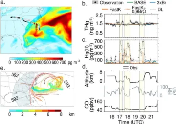
The mean THg concentrations for RF-09 calculated by the three simulations are between 1.38 and 1.42 ng m−3, and are
close to the mean of the observations (Fig. 7b). Between 16:00 and 19:00 UTC, the Hg(II) concentrations calculated with the FastK model (302 pg m−3) are closer to the
ob-servations (321 pg m−3) than with the BASE (127 pg m−3)
and 3×Br (253 pg m−3) models (Fig. 7c). However, between
19:00 and 19:30 UTC, the modeled Hg(II) concentrations for the three simulations are considerably lower (40–60 pg m−3) than the observed concentrations (300 pg m−3). The simu-lated RH (54 %) during this time was also higher than the observed RH (25 %). A comparison of the observed and modeled vertical profiles of isoprene (not shown) indicates an overestimate in the modeled local boundary layer depth,
Figure 7.Case study for RF-09 on 24 June 2013. Same as Fig. 6, ex-cept that we do not show BrO concentrations which were not mea-sured on this flight.
which could explain the difference between the model and the observations for this section of the flight.
For both RF-06 and RF-09, the GEOS-Chem simulations predict that the high observed Hg(II) concentrations were produced in the upper troposphere of the Pacific anticyclone. The upper troposphere is characterized by fast oxidation of Hg(0) to Hg(II) due to cold temperatures and higher Br con-centrations. Furthermore, the cloud-free conditions within the anticyclones prevent removal of Hg(II) by deposition and aqueous reduction, leading to accumulation of Hg(II) (Sect. 8).
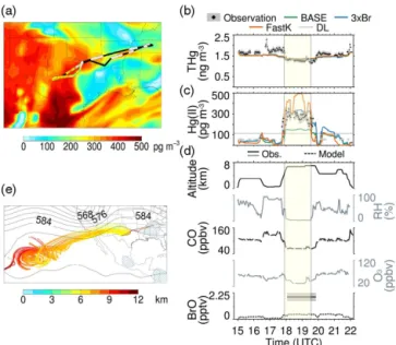
6.2 RF-16 (8 July 2013)
During RF-16, the aircraft flew to the South Carolina coast, with the goal of measuring the vertical distribution of mer-cury over the ocean (Fig. 8a). Of the eight constant alti-tude legs flown over the Atlantic, four were in the free tro-posphere, between 1.0 and 4.5 km, and four were in the marine boundary layer (MBL). THg concentrations showed a slight decrease from the MBL (1.58 ng m−3) to the top
of the vertical profile (1.37 ng m−3) (Fig. 8b). Hg(II) was
mostly BDL in the MBL, but was high in the free tropo-sphere reaching up to 680 pg m−3 with a mean
concentra-tion of 450 pg m−3(Fig. 8c). The Hg(II) DL on this flight was
91 pg m−3, and the Hg(II) filter was a cation exchange
mem-brane. The free-tropospheric air had a low concentration of CO (65 ppbv) and low RH (33 %) (Fig. 8d). The CHBr3
con-centration was about 1 pptv in the free tropospheric air, com-pared to about 2 pptv in the MBL. In consistency with the low RH and CHBr3, the HYSPLIT back trajectories show
Figure 8.Case study for RF-16 on 8 July 2013. Same as Fig. 6, except the background map (a)displays Hg(II) concentrations at 800 hPa for the FastK+0.9BrO pptv simulation. Also we add the FastK+0.9 ppt simulation as an orange dashed line in panels(b, c). O3concentrations were not available for this flight and BrO
concen-trations were below the instrument’s detection limit.
The simulated THg concentrations in the MBL (1.34– 1.38 ng m−3) are lower than the observations (1.58 ng m−3),
suggesting an underestimate in the ocean emission flux (Song et al., 2015) or an overestimate in the deposi-tion flux (Fig. 8b). None of the model simuladeposi-tions cap-ture the enhancements in Hg(II) observed between 17:00 and 18:15 UTC, and again between 19:30 and 20:15 UTC (Fig. 8c). During this flight, observed BrO concentrations re-mained below the instrument’s DL of 0.9 pptv, and the mod-eled BrO concentrations were 0.1–0.3 pptv. We performed an additional simulation increasing the modeled BrO con-centrations in the free troposphere of the Bermuda anticy-clone to 0.9 pptv (with a proportional increase in Br radical concentrations) for the FastK simulation (FastK+0.9BrO). The resulting Hg(II) concentrations along the flight track in-crease to 150–500 pg m−3, in better agreement with the
ob-servations (Fig. 8c). The oxidation of Hg(0) in this air mass was considerably faster than the 3×Br or FastK simulations, which suggests that the uncertainties in both the Br radical concentrations and in the oxidation rate constant can simul-taneously affect the overall bias in the modeled Hg(II) in cer-tain areas.
7 Links to previous studies
The above comparison of the simulated Hg(II) concentra-tions with the NOMADSS observaconcentra-tions shows that the Hg(0) oxidation based on the standard rate constants (Goodsite et al., 2004, 2012; Donohoue et al., 2006) and the GEOS-Chem calculated Br concentrations is too slow. Increasing the free tropospheric Br concentrations by a factor of 3 or consid-ering the higher rate constants of Ariya et al. (2002) leads to
significant improvement in the model results in the free tro-posphere compared to the NOMADSS observations. By con-trast, Weiss-Penzias et al. (2015) found that the GEOS-Chem simulated Hg(II) concentrations in the free troposphere were 2.5 times higher on average than the observed concentrations at five high-elevation sites in western USA and Taiwan. Dif-ferences in the instruments and models used in their study and ours make it difficult to directly compare our findings. Weiss-Penzias et al. (2015) used the Tekran®
2537-1130-1135 system, which can underestimate Hg(II) in the pres-ence of O3(Lyman et al., 2010; McClure et al., 2014). Their
GEOS-Chem model is based on the reaction kinetics de-scribed in Holmes et al. (2010) and does not include updates described in Sect. 2.3.3. Importantly, the rate constant for the dissociation of HgBr (Reaction R2) has since been corrected, and is now a factor of 10–20 higher than the previous value. The faster rate of dissociation of HgBr decreases the modeled Hg(II) concentration at 600 hPa by a factor of about 1.5.
The relatively high DL of the UW-DOHGS instrument makes the NOMADSS observations unsuitable for an evalua-tion of faster oxidaevalua-tion in the boundary layer. However, three previous studies in the tropical and mid-latitude MBL have reported similar findings that the standard Hg(0)+Br oxida-tion kinetics are too slow to reproduce the observed Hg(II) concentrations, as discussed below.
Sprovieri et al. (2010) observed the diurnal cycle in RGM concentrations over the Adriatic Sea with daily enhance-ments of 20–40 pg m−3 at midday. Using a box model, the
authors found that they could reasonably reproduce the ob-servations with the Ariya et al. (2002) rate constant for the Hg(0)+Br reaction (Reaction R1), but only if the HgBr ther-mal dissociation (Reaction R2) was neglected. In their study, Br was considered to be the sole second-step oxidant (Re-action R4). If HO2, NO2, and BrO were to be included as
second-step oxidants (Dibble et al., 2012), as we do in our FastK simulation, it would provide an additional pathway for the oxidation of HgBr to Hg(II), and partly overcome the slowing effect of the HgBr thermal dissociation.
In analyzing RGM observations over the Galapagos Is-lands in the equatorial Pacific, Wang et al. (2014) showed that the inclusion of HO2and NO2as second-step oxidants
in the Hg(0)+Br reaction scheme based on Goodsite et al. (2012) and Dibble et al. (2012) was necessary to simulate the observed magnitude of the midday peaks in RGM con-centrations. The box modeling study assumed peak daytime BrO concentrations of 0.2 pptv, which is similar to the an-nual average GEOS-Chem BrO concentration of 0.14 pptv. However, because of the uncertainties in the Tekran® 2537-1130-1135 system measurements, the actual concentrations of Hg(II) could possibly be higher than the observed con-centrations (Wang et al., 2014; Lyman et al., 2010; Ambrose et al., 2013).
the standard Br-initiated mechanism was insufficient to re-produce the rate of depletion of Hg(0) and showed that oxida-tion of Hg(0) by BrO, at a rate close to that reported by Spicer et al. (2002), was necessary to explain the loss of Hg(0). If the FastK kinetics are considered, the Br-initiated pathway by itself can explain a large fraction of observed depletion rate of Hg(0). Although the BrO oxidation pathway cannot be entirely ignored (as discussed in Sect. 5), its importance, in this case, would be much smaller than what was found by Tas et al. (2012). Overall, these MBL studies are consistent with our analysis of the NOMADSS free tropospheric ob-servations in implying much faster tropospheric oxidation of Hg(0) than currently assumed.
8 Implications of faster oxidation in the GEOS-Chem model
The global annual tropospheric mercury budgets for the three simulations are presented in Fig. 9. Despite faster oxidation in the 3×Br and FastK simulations, we maintain the same global burden of THg by increasing the Hg(II) reduction rate (Sect. 2.3.4). Thus, the lifetime of THg against deposition is similar in all three simulations (∼8.5 months). While we acknowledge that the modeled burden and lifetime of THg are affected by the uncertainty in the emission and deposition fluxes of mercury (Lin et al., 2006; Selin, 2009), we choose to maintain these in the three simulations because it allows us to focus on the model’s sensitivity to redox kinetics.
The tropospheric oxidation of Hg(0) to Hg(II) in-creases from 10 900 Mg a−1 in the BASE simulation, to
18 300 Mg a−1 for 3×Br (factor of 1.7 increase) and
42 100 Mg a−1 (factor of 3.9 increase) for the FastK
sim-ulation. The lifetime of Hg(0) against oxidation to Hg(II) decreases from 5 months in the BASE simulation to 2.8– 1.2 months in the 3×Br and FastK simulations. The tropo-spheric burden of Hg(II) increases by 33 % in the 3×Br sim-ulation and by 66 % in the FastK simsim-ulations.
Compared to the BASE simulation, the lifetime of Hg(II) against reduction decreases from 35 days (BASE simula-tion) to 19 days (3×Br) and 8 days (FastK) simulations, respectively. This results in faster cycling between Hg(0) and Hg(II). Globally, 48 % of the Hg(II) formed in the tro-posphere in the BASE simulation is reduced back to Hg(0) (Fig. 9a), whereas in the 3×Br and FastK simulations, that fraction increases to 68–88 % (Fig. 9b and c). The faster re-duction in the simulations with faster oxidation implies that reduction plays a predominant role in controlling the burden and distribution of Hg(II) in the atmosphere. In view of our poor understanding of Hg(II) reduction in the atmosphere (Subir et al., 2011), we suggest that further laboratory and field measurements be conducted to constrain this process.
In this study, we chose to increase the reduction rate of Hg(II) to maintain the global burden of THg when oxidation is enhanced in 3×Br and FastK simulations. An alternative
Figure 9. Annual global tropospheric budget of mercury in the (a)BASE,(b)3×Br, and(c)FastK simulations for 2013. The bur-dens are in units of Mg (106g) and the fluxes are in units of Mg a−1 (Mg per year).
Figure 10.Average concentration of Hg(II) at 450 hPa during NO-MADSS (1 June to 15 July 2013) for the(a)BASE,(b)3×Br, and (c) FastK simulations. The contours show the NCEP/NCAR Re-analysis 450 hPa geopotential height averaged over the same period (contour interval: 6 decameter). Panel(d)indicates the mean mod-eled vertical profiles of Hg(II) concentrations for regions marked as “Box 1” and “Box 2” for the three simulations (BASE: green, 3×Br: blue, FastK: orange).
Two processes maintain the high modeled Hg(II) con-centrations in the subtropical anticyclones. First, the anticy-clones are characterized by large-scale sinking motion which transports higher Hg(II) concentrations from the upper tropo-sphere where fast oxidation of Hg(0) results from higher Br concentrations and lower temperatures slowing the thermal dissociation of the HgBr intermediate (Reaction R2). The locations of the 450 hPa enhancements in Hg(II) concentra-tions displayed in Fig. 10 are thus largely associated with the descending branches of the Hadley circulation. Note that the model predicts larger Hg(II) concentrations in the South-ern Hemisphere subtropics where the winter Hadley circula-tion is stronger. Second, the sinking air in the anticyclones suppresses cloud formation and precipitation, thereby pre-venting loss of Hg(II) by reduction and wet deposition. This leads to efficient accumulation of Hg(II) in the subtropical anticyclones, even at lower altitudes. The model predicts low 450 hPa Hg(II) concentrations in regions in the tropics with high cloud cover and precipitation (such as the Western Pa-cific), and in regions with low insolation, such as the South-ern (winter) Hemisphere polar region.
The model simulates frequent episodes of high Hg(II) con-centrations at 6.5 km over Texas during the summer of 2013 (Fig. 11a). From 1 June to 15 July, simulated midday (noon– 3 p.m.) Hg(II) concentrations were higher than 250 pg m−3 for 15 days in the FastK simulation (3×Br: 12 days), two of which were the days when RF-06 and RF-09 were con-ducted. RF-10 also flew at 7 km (425 hPa) over northern Texas and Oklahoma (Fig. 1) on 27 June 2013, but observed Hg(II) concentrations remained BDL (DL: 134 pg m−3)
dur-ing the high altitude leg. The 3×Br and FastK modeled
Figure 11. (a)Modeled time series of midday (noon–3 p.m.) Hg(II) concentrations at 6.5 km altitude over Texas (white rectangle shown in panelsb, c) for the three GEOS-Chem simulations (BASE: green, 3×Br: blue, FastK: orange) for 1 June–15 July 2013 and the mean and standard deviations of Hg(II) observations at 6–7 km over Texas for RF-06, RF-09 and RF-10.(b)Mean midday FastK Hg(II) con-centrations and winds at 6.5 km altitude for the 10 highest FastK Hg(II) concentrations from the time series in panel(a).(c)Mean midday FastK Hg(II) concentrations for the 10 days with the lowest Hg(II) concentrations.
Hg(II) concentrations over this region during RF-10 were 136 and 208 pg m−3, respectively, significantly lower than
those simulated for RF-06 and RF-09. The highest Hg(II) at 6.5 km over Texas and Oklahoma occurs when the wind over the southern US is southwesterly (Fig. 11b) transporting Hg(II) from the semi-permanent Pacific anticyclone, whereas the lowest concentrations occur when the transport is from the north (Fig. 11c). Our results suggest that the transport of Hg(II) produced in the Pacific anticyclone could be an impor-tant source of Hg(II) over southeastern US, potentially influ-encing wet deposition in the region if these high Hg(II) air masses are exposed to deep convection.
9 Conclusions
the bottom 1 km (1.54 ng m−3), and lower concentrations
be-tween 6 and 7 km (1.38 ng m−3) in the atmosphere.
During NOMADSS, the mean Hg(II) concentrations observed above the instrument’s limit of detection was 212 (±112) pg m−3. Using the robust regression on order statistics procedure, the estimated mean Hg(II) concentra-tion for all observaconcentra-tions was 110 (±103) pg m−3. The highest
Hg(II) concentrations, 300–680 pg m−3, were seen at 5–7 km
altitude during two flights over Texas and at 1–3 km during one flight over the Atlantic Ocean. These high Hg(II) con-centrations were associated with clean subsiding air masses originating in the upper troposphere within the Pacific or At-lantic anticyclones. The low temperatures and high concen-trations of the bromine radical in the upper troposphere lead to faster oxidation of Hg(0), while the lack of removal from in-cloud reduction or wet deposition in the dry anticyclones lead to efficient accumulation of Hg(II).
We used the GEOS-Chem model to evaluate the oxidation kinetics and interpret these observations. The modeled THg concentrations are in close agreement with the observations, reproducing the horizontal and vertical distribution of THg. The simulated Hg(II) concentrations, on the other hand, are a factor of 2.2 lower than the observed concentrations. We attribute this systematic bias to an underestimate in the mod-eled oxidation of Hg(0) to Hg(II).
We perform two additional simulations with (i) three times the Br radical concentrations between 45◦N and 45◦S and between 750 hPa and the tropopause (3×Br), and (ii) a faster Hg(0)+Br oxidation rate constant (FastK). The model performance improves with both these simulations, espe-cially above 5 km altitude and in air masses with low RH (<35 %) and low CO (<75 ppbv), where some of the highest Hg(II) concentrations were observed. For these air masses, the Hg(II) concentrations simulated with the 3×Br (162±104 pg m−3) and the FastK (208±144 pg m−3) mod-els are 60–100 % higher than the BASE simulation (99±
48 pg m−3) and in closer agreement with the observations
(239±141 pg m−3). In addition to oxidation of Hg(0) by Br
(BASE case), we considered the effect of including O3and
OH as oxidants, but found that the high Hg(II) concentrations observed at 5-7 km could not be reproduced. We also ex-amined the effect of adding the Hg(0)+BrO reaction to the BASE simulation, and found that the model underestimate of Hg(II) at 5-6 km persisted. Our modeling study suggests that the NOMADSS observations are most consistent with the 3×Br simulation and the FastK simulation, however we note that the relative importance of the different oxidation pathways cannot be ascertained before the chemical forms of Hg(II) in the atmosphere have been identified.
Faster oxidation decreases the lifetime of Hg(0) against oxidation from 5 months in the BASE simulation to 2.8 months with the 3×Br simulation, and to 1.2 months with the FastK simulation. To maintain the global THg burden, the faster modeled Hg(0) oxidation is balanced by an increase in the modeled Hg(II) reduction rates. The contribution of
duction to the overall loss of Hg(II) (by deposition and re-duction) increases from 48 % in the BASE simulation to 68 and 88 % in the 3×Br and the FastK simulations, respec-tively, implying a greater importance of reduction to chem-istry of mercury in the atmosphere. In the subtropical anticy-clones, the 3×Br and FastK simulations predict a 3 to 5-fold enhancement in Hg(II) concentrations at 450 hPa relative to the global average Hg(II) concentration. These subtropical anticyclones are dry, cloud-free regions which provide ideal conditions for accumulation of Hg(II). The high Hg(II) in the Pacific anticyclone is periodically transported over southern US during summer and could be an important source of mer-cury wet deposition in the region. Future measurements in the subtropical anticyclones can help us gain deeper insights into the pathways of Hg(0) oxidation in the atmosphere.
The Supplement related to this article is available online at doi:10.5194/acp-16-1511-2016-supplement.
Acknowledgements. This material is based upon work supported by the National Science Foundation under grant no. 1217010 to D. A. Jaffe, L. Jaeglé and N. E. Selin, grant no. 1215712 to J. Stutz, and grant no. 1216743 to C. A. Cantrell and R. L. Mauldin III. The authors thank participants from National Center for Atmospheric Research’s Earth Observing Laboratory and Research Aviation Facility for their support in the planning and execution of the NOMADSS campaign.
Edited by: A. Dastoor
References
Ambrose, J. L., Lyman, S. N., Huang, J., Gustin, M. S., and Jaffe, D. A.: Fast time resolution oxidized mercury measure-ments during the Reno Atmospheric Mercury Intercomparison Experiment (RAMIX), Environ. Sci. Technol., 47, 7285–7294, doi:10.1021/es303916v, 2013.
Ambrose, J. L., Gratz, L. E., Jaffe, D. A., Campos, T., Flocke, F. M., Knapp, D. J., Stechman, D. M., Stell, M., Weinheimer, A., Cantrell, C., and Mauldin, R. L.: Mercury emission ratios from coal-fired power plants in the southeastern U.S. dur-ing NOMADSS, Environ. Sci. Technol., 49, 10389–10397, doi:10.1021/acs.est.5b01755, 2015.
Amos, H. M., Jacob, D. J., Holmes, C. D., Fisher, J. A., Wang, Q., Yantosca, R. M., Corbitt, E. S., Galarneau, E., Rutter, A. P., Gustin, M. S., Steffen, A., Schauer, J. J., Graydon, J. A., Louis, V. L. St., Talbot, R. W., Edgerton, E. S., Zhang, Y., and Sunder-land, E. M.: Gas-particle partitioning of atmospheric Hg(II) and its effect on global mercury deposition, Atmos. Chem. Phys., 12, 591–603, doi:10.5194/acp-12-591-2012, 2012.