www.atmos-meas-tech.net/9/3769/2016/ doi:10.5194/amt-9-3769-2016
© Author(s) 2016. CC Attribution 3.0 License.
Recommendations for processing atmospheric attenuated
backscatter profiles from Vaisala CL31 ceilometers
Simone Kotthaus1, Ewan O’Connor1,2, Christoph Münkel3, Cristina Charlton-Perez4, Martial Haeffelin5, Andrew M. Gabey1, and C. Sue B. Grimmond1
1Department of Meteorology, University of Reading, Reading, RG6 6BB, UK 2Finnish Meteorological Institute, 00101 Helsinki, Finland
3Vaisala GmbH, 22607 Hamburg, Germany
4Met Office, Meteorology Building, University of Reading, Reading, RG6 6BB, UK
5Institute Pierre Simon Laplace, Centre National de la Recherche Scientifique, École Polytechnique, 91128 Palaiseau, France
Correspondence to:Simone Kotthaus ([email protected])
Received: 14 March 2016 – Published in Atmos. Meas. Tech. Discuss.: 29 March 2016 Revised: 12 July 2016 – Accepted: 20 July 2016 – Published: 17 August 2016
Abstract. Ceilometer lidars are used for cloud base height detection, to probe aerosol layers in the atmosphere (e.g. de-tection of elevated layers of Saharan dust or volcanic ash), and to examine boundary layer dynamics. Sensor optics and acquisition algorithms can strongly influence the observed attenuated backscatter profiles; therefore, physical interpre-tation of the profiles requires careful application of cor-rections. This study addresses the widely deployed Vaisala CL31 ceilometer. Attenuated backscatter profiles are stud-ied to evaluate the impact of both the hardware generation and firmware version. In response to this work and discus-sion within the CL31/TOPROF user community (TOPROF, European COST Action aiming to harmonise ground-based remote sensing networks across Europe), Vaisala released new firmware (versions 1.72 and 2.03) for the CL31 sensors. These firmware versions are tested against previous versions, showing that several artificial features introduced by the data processing have been removed. Hence, it is recommended to use this recent firmware for analysing attenuated backscatter profiles. To allow for consistent processing of historic data, correction procedures have been developed that account for artefacts detected in data collected with older firmware. Fur-thermore, a procedure is proposed to determine and account for the instrument-related background signal from electronic and optical components. This is necessary for using atten-uated backscatter observations from any CL31 ceilometer. Recommendations are made for the processing of attenuated
backscatter observed with Vaisala CL31 sensors, including the estimation of noise which is not provided in the standard CL31 output. After taking these aspects into account, attenu-ated backscatter profiles from Vaisala CL31 ceilometers are considered capable of providing valuable information for a range of applications including atmospheric boundary layer studies, detection of elevated aerosol layers, and model veri-fication.
Copyright statement
The works published in this journal are distributed under the Creative Commons Attribution 3.0 License. This license does not affect the Crown copyright work, which is re-usable under the Open Government Licence (OGL). The Creative Commons Attribution 3.0 License and the OGL are interop-erable and do not conflict with, reduce or limit each other. ©Crown copyright 2016
1 Introduction
originally developed as “cloud base recorders”, attenuated backscatter profiles from ceilometers can also provide in-formation on rainfall (Rogers et al., 1997), in-formation and clearance of fog (Haeffelin et al., 2010), drizzle properties (when combined with cloud radar; O’Connor et al., 2005), and for the study of aerosols, including elevated layers of Saharan dust (Knippertz and Stuut, 2014), biomass burning (Mielonen et al., 2013) or volcanic ash (e.g. Marzano et al., 2014; Nemuc et al., 2014; Wiegner et al., 2012), and par-ticles dispersed within in the atmospheric boundary layer (ABL) (Tsaknakis et al., 2011). Using aerosols as a tracer, boundary layer dynamics, including mixing height and the formation of residual layers, can be inferred from ceilome-ter attenuated backscatceilome-ter observations (e.g Münkel et al., 2007; Stachlewska et al., 2012; Selvaratnam et al., 2015). As they can operate automatically for long periods with-out maintenance or human intervention even in extreme cli-mates (Bromwich et al., 2012), they are widely deployed op-erationally by national meteorological services (NMS, e.g. http://www.dwd.de/ceilomap) and long-term research cam-paigns (e.g. http://micromet.reading.ac.uk).
Although ceilometers are regarded as the most basic auto-matic lidars (Emeis, 2010), they detect the location and ex-tent of aerosol layers and can be used to derive the aerosol backscatter coefficient, provided signal-to-noise ratio (SNR) is sufficient and a careful calibration is applied (e.g. Jenoptik CHM15K; Heese et al., 2010; Wiegner et al., 2014). Obser-vations from ceilometers are highly valuable for the evalua-tion of numerical weather predicevalua-tion (NWP) and air-quality models (Emeis et al., 2011b) and are increasingly used in forecast verification. Several NMS and research centres are currently evaluating the potential of using ceilometer profile observations for data assimilation (Illingworth et al., 2015).
This wide range of applications requires careful qual-ity control of the observed attenuated backscatter to en-sure reliable data for analysis. The European COST Action TOPROF (http://www.toprof.imaa.cnr.it/) works in close col-laboration with E-Profile (http://www.eumetnet.eu/e-profile) to develop protocols for quality assurance and quality con-trol (QAQC; Illingworth et al., 2015) of observations from automatic lidars and ceilometers (ALCs). The E-Profile pro-gramme of the Network of European Meteorological Ser-vices (EUMETNET) aims to facilitate the exchange of obser-vational data by harmonising the ALC networks across Eu-rope. As ceilometers are manufactured by several companies, the sensor optics, hardware components, and software algo-rithms may differ significantly. Discussions in the TOPROF community have revealed the importance of a detailed un-derstanding of instrument specifics to identify the neces-sary processing steps enabling appropriate interpretation and harmonisation of the final data products. For example, the extensive CeiLinEx2015 intercomparison campaign (http: //www.ceilinex2015.de) was devised by TOPROF members to evaluate attenuated backscatter and cloud base height products from a range of ceilometer models from several
manufacturers (including Lufft/Jenoptik, Campbell Scien-tific, and Vaisala). This study addresses the commonly de-ployed Vaisala CL31 ceilometer. Earlier Vaisala ceilome-ter models include LD40 and CT25K; the CL51 is the most recent model.
Emeis et al. (2011a) report that attenuated backscatter from Vaisala CL31 ceilometers portrays structures in the ABL consistent with temperature and humidity profiles ob-served by radiosondes and a sodar RASS system. Initial eval-uation of CL31 attenuated backscatter observations for quan-titative aerosol analysis (Sundström et al., 2009) suggests accuracy might be sufficient in the ranges near the instru-ment if certain systematic artefacts found in the profiles can be removed or accounted for. McKendry et al. (2009) find that, under clear-sky conditions, the CL31 has the capabil-ity to “detect detailed aerosol layer structure (such as fire or dust plumes) in the lower troposphere” that is consistent with the aerosol structure detected by an aerosol research lidar (CORALNet-UBC). However, comparing a Vaisala LD40 and two CL31 ceilometers, Emeis et al. (2009) show that attenuated backscatter may vary distinctly between these sensors. The differences found cannot be explained by a lack of absolute calibration as they are manifested in ver-tical structures rather than as a simple offset. Instrument-specific signatures may have implications for the representa-tion of ABL structures. Emeis et al. (2009) state “internally generated artefacts from the instrument’s software” could play a role, but they refrain from providing further details. While software-related artefacts might contribute to the dif-ferences, the discrepancy between the attenuated backscatter profiles observed by the two CL31 sensors tested (Emeis et al., 2009) might also be explained by the hardware-related (electronic or optical) background signal. Recent work on a Halo Doppler lidar suggests such background signal features could be corrected for during post-processing (Manninen et al., 2016).
et al. (2009) evaluate the applicability of CL31 observations for quantitative aerosol measurements and conclude that the artefacts in the range gates near the instrument are a major source of uncertainty. Van der Kamp (2008) smooths out sys-tematic artefacts by strong vertical averaging; however, this removes the possibility of identifying any atmospheric fea-tures close to the surface.
Various techniques have been developed to infer the mix-ing height from the shape of the attenuated backscatter pro-files from ceilometers (Emeis et al., 2008; Haeffelin et al., 2012). While detection algorithms vary, all methods exploit the fact that aerosol concentrations (and atmospheric mois-ture if boundary layer clouds are absent) are typically signif-icantly higher in the ABL compared to the free atmosphere above. This causes a distinct decrease in attenuated backscat-ter at the boundary layer top, provided that the SNR is suffi-ciently large up to this height.
A series of studies have successfully used CL31 obser-vations to detect mixing height (e.g. Münkel et al., 2007; van der Kamp and McKendry, 2010; Eresmaa et al., 2012; Sokół et al., 2014; Tang et al., 2016), often reporting an increased performance under convective conditions that en-sure the backscattering aerosols are well dispersed. However, Eresmaa et al. (2012) report that fitting an idealised profile to the observed attenuated backscatter from a CL31 may be challenging where noise levels are high. As the CL31 op-erates with a very low-powered laser, its noise levels may be higher than that found for other ALC systems (cf. Jenop-tik CHM15K; Haeffelin et al., 2012). Madonna et al. (2015) evaluate the profiling ability of several ALCs from differ-ent manufacturers (i.e. Jenoptik CHM15K, Vaisala CT25K, and Campbell CS135s) against a MUSA advanced Raman lidar during night-time. They conclude that the attenuated backscatter coefficient generally is in good agreement with the reference measurement for the CHM15K, while the CS135s shows good agreement only for small values and the CT25K tends to underestimate, which may be related to the overall lower SNR of the latter two sensors. If noise levels are too high within the ABL, as reported e.g. by Haeffelin et al. (2012) for a case study using a Vaisala CL31 ceilometer at the SIRTA site near Paris, the signal might not be sufficient to detect the top of the ABL. De Haij et al. (2006) apply an SNR threshold to restrict observations from a Vaisala LD40 ceilometer to be used for mixing height detection. Such filter-ing based on SNR diagnostics presents a useful tool to dif-ferentiate measurements containing significant atmospheric signal from observations dominated by instrument noise and atmospheric noise induced by solar radiation.
Neither the SNR nor the noise inherent in each profile is provided in the output of ALCs. Xie and Zhou (2005) pro-pose a method for SNR calculations for lidar observations whereby the signal profile is approximated by a linear fit to the readily averaged profile along set range bins and as-signing the deviations from that fit to the noise. Markowicz et al. (2008) apply this method to observations of a Vaisala
CT25K averaged over 200 s. These SNR values indicate that the observations are only reliable within the ABL (absence of clouds) and it is stated that an SNR=10 marks “a
limit-ing value of detection” (Markowicz et al., 2008). Assumlimit-ing there are no temporal variations in the atmosphere probed by several consecutive observations (e.g. over a few minutes), the standard deviation at each range gate could be used as a noise estimate of the respective average if high-temporal-resolution measurements are recorded (Xie and Zhou, 2005). Assuming the noise is range-invariant before the range cor-rection, a noise estimate for the whole profile could be es-timated based on observations where the signal contribution is negligible, e.g. based on the topmost range gates under the absence of high clouds and aerosol layers. Heese et al. (2010) use the highest range gates to calculate a noise value for each profile for a Jenoptik CHM15K, assuming the signal noise follows Poisson statistics as typically assumed for photon counting detectors. Vaisala sensors operate with an avalanche photodiode (APD), so that the noise cannot be interpreted as a counting error. The SNR increases significantly when high-resolution observations are averaged over certain time and/or range windows. Using a Gaussian smoothing method on ob-servations of a Jenoptik CHM15K, Stachlewska et al. (2012) find that the SNR significantly increases if the width of range windows is increased linearly. However, they remark that this may result in extensive computing time. In addition, exces-sively large smoothing windows may reduce the detectability of sharp features (Haeffelin et al., 2012).
Despite the evidence that attenuated backscatter profiles are a complex data product that might have to be care-fully evaluated before being used to draw conclusions on the probed atmosphere, no guidelines are available to en-sure systematic QAQC. This study documents the important processing steps that should be considered when analysing attenuated backscatter profiles from Vaisala CL31. Observa-tions from three ALC networks (Sect. 2) are used to illus-trate relevant data processing aspects (Sect. 3). Depending on the firmware version, the CL31 instrument internal process-ing may introduce certain artefacts that should be accounted for if the attenuated backscatter is required for analysis. It is shown how the signal strength can be used for quality as-surance (Sect. 4) and findings are summarised in the form of recommendations for the processing of CL31 profile obser-vations (Sect. 5).
2 Instrument description
Gaussian low-pass filtering of 3 MHz by the instrument ex-tends and shapes the pulse response. Different vertical res-olutions can be achieved depending on the sample rate. For example, a sample rate of 15 MHz is required to achieve a range resolution of 10 m, where the first observation reported at 10 m is backscattered signal for 5–15 m from the ceilome-ter. Every 2 s, 214laser pulses are emitted with a frequency of 10 kHz, which takes about 1.64 s. After this period there is an idle time of 0.36 s used to perform the cloud base detec-tion algorithm before the next set of 214laser pulses is emit-ted. After a certain number of gates have been sampled, the firmware slightly changes operation mode; thus, regions of increased noise are introduced into the backscatter profiles at two ranges:∼4940 and∼7000 m. Samples collected during the 2 s intervals are averaged over certain internal intervals to create the reported signal at a rate defined by the reporting interval selected by the user (2–30 s). The internal averaging interval is specific to the firmware (see below).
The spectral wavelength of the laser diode used in the Vaisala CL31 is 905±10 nm at 298 K, as stated by the laser manufacturer. Vaisala finds the uncertainty of the nominal centre wavelength to be well below 10 nm. Typical spec-tral width (full width at half maximum, FWHM) is 4 nm. Lasers produced from the same wafer agree in terms of the centre wavelength, but the exact centre wavelength is un-known to the user. For a specific laser the centre wavelength is slightly temperature dependent (0.3 nm K−1). The CL31 system heater near the laser transmitter serves to stabilise the laser temperature in cold environments. Further, both win-dow transmission and laser pulse energy can have an im-pact on the attenuated backscatter signal. The laser heat sink temperature (denoted in the CL31 output as the “laser tem-perature”), window transmission, and laser pulse energy are therefore monitored and reported continuously. Status infor-mation (i.e. diagnostics, warnings, and alarms) is included in the data message, which helps to identify whether main-tenance is required (e.g. window needs cleaning, transmitter is failing). In addition to the detected cloud base height, the CL31 can be set to report a profile of range-corrected “atten-uated backscatter”. However, as these values lack absolute calibration (see Sect. 4.1), observations are here referred to as the “reported range-corrected signal” (RCS; for details on range correction see Sect. 3.2).
The detector of the CL31 responds to the backscattering of the laser pulse from molecules, aerosols, rain drops, and both liquid and ice cloud particles. It also responds to noise originating from both external (e.g. daytime solar radiation) and internal (e.g. electronic) sources. The hardware-related noise is larger than the Rayleigh signal associated with clear air so that the latter is too small to be distinguished. Vaisala states that the variance of the electronic noise signal is range independent. The background light from solar radiation in-creases the current through the APD, but as the amplifiers are AC coupled, the relatively slowly varying solar signal (almost DC) does not get to the A/D converter. (The
AC-Table 1. Internal averaging interval applied in different CL31
firmware versions as a function of rangerand reporting interval.
Reporting interval
Firmware version Range (m) 2 s 3–4 s 5–8 s > 8 s
< 1.72, 2.01, 2.02 r< 600 2 s 4 s 8 s 16 s
600≤r< 1200 4 s 4 s 8 s 16 s
1200≤r< 1800 8 s 8 s 8 s 16 s
1800≤r< 2400 16 s 16 s 16 s 16 s
r≥2400 30 s 30 s 30 s 30 s
1.72, 2.03 r> 0 30 s 30 s 30 s 30 s
coupling time constant is 1 ms; i.e. the AC coupling works as a high-pass filter with 159 Hz corner (−3 dB) frequency.)
This filtering results in a variable zero-bias level (i.e. noise has negative and positive values) that accounts for temporal variations in the atmospheric background signal. While the AC coupling removes the low frequency signal from vary-ing solar radiation, the latter still increases signal noise (shot noise in APD due to DC current). For short data acquisition intervals, backscatter values can be below 0. Electronic noise is also a function of system properties (e.g. detector tem-perature, transmitter lens area; Gregorio et al., 2007; Vande Hey, 2014) and can therefore be analysed by the manufac-turer prior to field deployment. Heaters provide partial ther-mal stabilisation of the laser and detector system in cool or cold conditions.
The Vaisala CL31 firmware has been modified over time along with certain developments in the hardware, i.e. the receiver (CLR) and engine board (CLE) where the internal processing takes place. These updates have re-sulted in the creation of a range of firmware versions. For CLE311+CLR311, the firmware versions 1.xx are used, while sensors with CLE321+CLR321 run firmware ver-sions 2.xx. Changing the ceilometer transmitter (CLT) gen-eration is not connected to a change in firmware. The internal averaging interval differs slightly with firmware version (Ta-ble 1). In Vaisala CL31 firmware versions below 1.72 and versions 2.01 and 2.02, the internal averaging interval is set to 16 s for range gates below 2400 m if the reporting interval is greater than 8 s. For reporting intervals between 5 and 8 s, the internal averaging interval is set to 8 s below 1800 m and 16 s between 1800 and 2400 m. For reporting intervals below 5 s internal averaging below 1200 m is 4 s; only for the min-imum reporting interval of 2 s is internal averaging set to 2 s below 600 m. Above 2400 m, the internal averaging is 30 s for all reporting intervals. In firmware 1.72 and 2.03, the in-ternal averaging interval is 30 s for the entire profile and does not change with reporting interval (Table 1). If a reporting interval is selected that is shorter than the internal averaging interval, consecutive profiles overlap in time and are hence not completely independent.
Table 2.Vaisala CL31 ceilometer specifications of sensor hardware, firmware, H2 noise setting, and resolution selected by the user. The term “H2” is discussed in Sect. 3.2.
Sensor ID Network Ceilometer engine board/receiver/transmitter Firmware version H2 Resolution
(time, range)
A LUMO CLE311/CLE311/CLT311 1.56, 1.61, 1.71 On 15 s, 10 m
CLE311/CLE311/CLT321 1.71, 1.72 On 15 s, 10 m
B LUMO CLE311/CLE311/CLT311 1.61 On 15 s, 10 m
CLE311/CLE311/CLT321 1.61, 1.71, 1.72 On 15 s, 10 m
C LUMO CLE321/CLE321/CLT321 2.01, 2.02, 2.03 On 15 s, 10 m
D LUMO CLE321/CLE321/CLT321 2.01, 2.02, 2.03 On 15 s, 10 m
W Met Office CLE311/CLE311/CLT311 1.71 Off 30 s, 20 m
S Meteo France CLE321/CLE321/CLT321 2.01 On 30 s, 15 m∗
∗Block averages of the recorded data (2 s, 5 m) are used for sensor S.
acquisition and processing of Vaisala CL31. The Lon-don Urban Micromet Observatory (LUMO; http://micromet. reading.ac.uk) is a measurement network collecting ob-servations of many atmospheric fields to investigate cli-mate conditions within and around Greater London, UK (for interactive map see http://www.met.reading.ac. uk/micromet/LUMA/Network.html). The Met Office oper-ates an ALC network (http://www.metoffice.gov.uk/public/ lidarnet/lcbr-network.html) across the UK with different manufacturers/models, including Vaisala CL31. A CL31 is operated by Meteo France at the SIRTA site at Palaiseau, France, for atmospheric research activities (Haeffelin et al., 2005; http://www.sirta.fr). Four sensors from the LUMO net-work in central London, one Met Office sensor located 60 km west of central London, and the Meteo France/SIRTA sen-sor are used here.
Long-term observations are available from four CL31 ceilometers with different generations of hardware and var-ious firmware versions. Over time, the LUMO network firmware versions have changed from the first LUMO sen-sor deployed in 2006 with version 1.56 (Table 2). Sensen-sors A and B are the old hardware generation with the CLE311 board, as is the Met Office sensor W, while LUMO sensors C and D and the SIRTA sensor S have engine boards CLE321. For both sensors A and B the transmitter has been upgraded from CLT311 to CLT321 during their operation, and for sen-sor S the transmitter CLT321 was replaced by a spare part of the same generation. While the LUMO sensors are set to ac-quire data every 15 s with a vertical resolution of 10 m, data from the Met Office ceilometer have a resolution of 30 s and 20 m, and the SIRTA ceilometer captures data every 2 s with a range resolution of 5 m. Analysis presented here uses block averages over 30 s and 15 m of the SIRTA ceilometer data.
3 Corrections
3.1 Background correction
The backscattered signal detected by an ALC generally con-sists of actual signal contributions from atmospheric atten-uation, the atmospheric background signal associated with scattered solar radiation, and the instrument-related back-ground signal (Cao et al., 2013). Here, “backback-ground signal” is used to describe systematic contributions from solar radia-tion or instrument components (including hardware and soft-ware). The CL31 measurement design accounts for the tem-poral noise bias induced by varying solar radiation by intro-ducing a variable zero-bias level (Sect. 2). The atmospheric background signal still contributes to the noise in the profile. On average, the RCS (labelled “range and sensitivity nor-malised attenuated backscatter” in CL31 output) is inherently corrected for the impact of atmospheric background signal Pbga(r) and only the instrument-related background signal Pbgi(r)needs to be accounted for to derive the background-corrected signalPˆ(for ALC terminology see also Mattis and
Wagner, 2014). Given that the time dependence of the data acquisition is linked to the spatial domain, the instrument-related background signal may vary with range, while sta-bilisation procedures (e.g. heaters) aim to reduce its tempo-ral variability. Here, as tempotempo-ral signal variations due to the solar background light are removed, the remaining temporal variations are considered to represent noise both from hard-ware and atmospheric background signal.
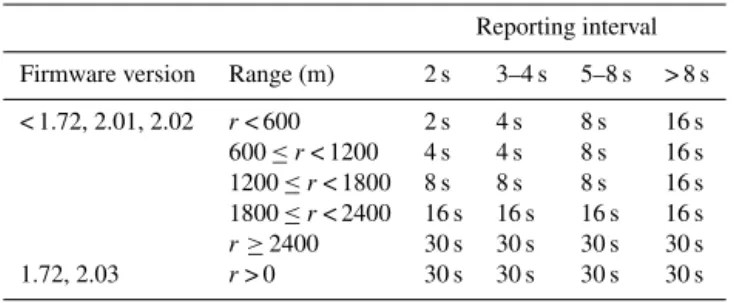
Figure 1.Range histograms for 24 h of observations from Vaisala CL31 ceilometers operating with firmware versions (1.56–2.03) on different
clear-sky days. Sensor ID in brackets (see Table 2 for settings, e.g. H2=off for sensor W). Rows: range histograms in arbitrary units (a. u.)
of(a)signalP,(b)range-corrected signal reported RCS=P·r2, and(c)range-corrected, background-corrected signalPˆ·r2(Sect. 3.1).
Median profiles (solid lines) are included in(b)and(c). The H2 setting (Sect. 3.2) allows switching off of the range correction above 2400 m
for regions with no clouds present.
that the background signal of the respective data is biased and no longer centred on 0 (e.g. data collected with version 1.71 have more negative than positive values). This is applied to improve detection of cloud base height as it amplifies differ-ences between the signal backscattered from cloud droplets and areas with low concentration of atmospheric scatterers where observations are dominated by noise. Increasing this difference facilitates visual interpretation of clouds based on the backscattered signal. Hereafter, this bias is referred to as “cosmetic shift” Pcs(r). Thus, to derive the entirely background-corrected signal from CL31 output, the com-plete background signalPbg, composed of range-dependent, instrument-related background signal Pbgi(r) and the cos-metic shiftPcs(r), needs to be accounted for
ˆ
P (r)=P (r)−Pbg(r)=P (r)−Pbgi(r)−Pcs(r) . (1)
For data collected with firmware 1.72 or 2.03, no cosmetic shift is incorporated (Pcs(r)=0), so that the complete back-ground correction is represented by the range-dependent, instrument-related background signal (Pbg(r)=Pbgi(r)). The impact of background signal and cosmetic shift on the reported signal is illustrated using observations from differ-ent clear-sky days (no elevated dust, aerosol layers, or cir-rus) from CL31 sensors running a range of firmware versions (Fig. 1a). Under such conditions the only source of atmo-spheric signal above the ABL is very weak molecular and aerosol scattering. In practice, molecular scattering at the in-strument wavelength is very weak, typically below the sen-sitivity of the instrument (Sect. 2), so that profiles consist only of the average total background signal and the noise. As
the atmospheric background signal only contributes to the noise, no systematic differences in the shape of the observed profiles would be expected and obvious departures from 0 can be associated with data acquisition and processing, i.e. instrument-related background signal and potential cosmetic shift.
A suitable method to identify discrepancies in the profile shape is to create signal-range histograms (Fig. 1a) using 24 h (or more) of data. The most obvious effect revealed by the range histograms is a step change in the width of the dis-tributions at 2400 m evident for all firmware versions, apart from 1.72 and 2.03. This step change is introduced by the averaging of the sampled signal that is applied internally by the instrument’s firmware (Sect. 2, Table 1). The decrease in averaging time for range gates < 2400 m performed for ear-lier firmware increases the signal noise (see Sect. 4.2). Data acquired with version 1.72 or 2.03 are more consistent across all range gates as the whole profile is treated equally with an internal averaging interval of 30 s.
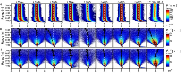
trans-Figure 2.SignalP(derived from reported signal by reverting range correction) observed with Vaisala CL31 sensors operating with(a, b)
en-gine board CLE311+receiver CLR311 (A, B) and(c, d, e)CLE321+CLR321 (C, D, S), respectively (Table 2);(a–d)January 2011–
April 2016 and(e)May 2015–April 2016 for range > 2400 m. Observations (4 h around midnight, 22:00–02:00 UTC) are hourly means
of profiles when clouds detected for < 10 % of the hour, no fog, average window transmission > 80 %, laser pulse energy > 98 %, and data availability > 90 %. Left: top axis shows firmware updates (version 1.71, then 1.72 for sensors A and B; versions 2.02, then 2.03 for C and D; version 2.01 for S) and hardware changes/upgrades (transmitter CLT311 replaced by CLT321 for sensors A and B; CLT321 replaced by a new CLT321 for sensor S). Right: median profiles (with IQR shading) of all selected observations grouped by firmware version and
transmitter, withNindicating the number of profiles.
mission is reasonable (> 80 % on average), laser pulse en-ergy is high (> 98 % of nominal enen-ergy), and sufficient data are available (> 90 % of the hour; data gaps may occur due to maintenance or problems with data acquisition such as power cuts). Only range gates > 2400 m are analysed to avoid the impact of changing internal averaging intervals (Sect. 2) at this critical range (Fig. 1a) and to minimise the signal from the ABL (unlikely to extend above 2400 m over London around midnight). Median vertical profiles (with interquartile range (IQR) shading) are displayed for common setup condi-tions (Fig. 2, right), i.e. grouped by combinacondi-tions of sensor, firmware, and transmitter (CLT). Engine board and receiver were not changed for any of the sensors during their opera-tion.
The night-time profile climatology (Fig. 2) reveals a small temporal variability with a seasonal cycle (ampli-tude∼50 %) that indicates a temperature dependence of the instrument-related background signal. Several features ap-pear distinct in the spatial domain (Fig. 2) at certain range gates. For all sensors and firmware versions, a discontinuity is evident just below 5000 m and at around 7000 m. These regions of increased noise are introduced by the data storage
procedure (Sect. 2). Changing hardware components affects the instrument-related background signal even if the same model is swapped in. For example, exchanging the transmit-ter of sensor S by a part of the exact same model (CLT321 exchanged in September 2015, Fig. 2e) resulted in a clear increase of the background signal below about 4000 m. As it cannot be guaranteed that the new transmitter has the ex-act same charex-acteristics as the one replaced (Sect. 2), a slight change in wavelength might explain this shift.
en-Figure 3.Long-term median vertical profiles of range-dependent, instrument-related backgroundPbgifor Vaisala CL31 sensors (Table 2).
Statistics are based on hourly mean profiles (r> 2410 m) of the signalP (derived from reported signal by reverting range correction) observed
around midnight (same data as Fig. 2). Ceilometers A and B operated with firmware 1.61, 1.71, or 1.72 and transmitter type CLT311 or CLT321, respectively; ceilometers C and D operated with CLT321 and firmware 2.01, 2.02, and 2.03; ceilometer S operated with firmware
2.01 and CLT321.(a)Median profiles for each sensor calculated separately by firmware version for sensors A and B, all of which are
combined for C and D (2.xx) due to their similarity.(b)As in(a)for sensors A, C, B, and D but also separating by ceilometer transmitter
CLT and laser heat sink temperature combinations (see legend); laser heat sink temperature (reported by the ceilometer as laser temperature)
is used to subdivide profiles into three classes (Tlaser < 303 K, 303 K≤Tlaser< 308 K, andTlaser≥ 308 K).(c)As in(b)but for selected
profiles (solid lines, A and B with 1.71 and 1.72; C and D with 2.03) and their respective background profiles as determined by a 30 min
termination hood measurement at the same setting and laser heat sink temperature class (thick lines). (d)As in(c)but range-corrected.
(e)As in(d)but zoomed into the range < 3000 m. Number of hourly mean profilesN(h) available for each combination of sensor, firmware,
transmitter type CLT, and laser heat sink temperature is listed in the legend. Profiles are smoothed vertically with a moving average over a window of 210 m; only for profiles from sensor B is a smoothing window of 310 m used.
tirely constant over the course of a day because it is slightly affected by attenuation by clouds and ABL particles. As shown, this ripple is sensor specific (e.g. higher frequency detected for sensor B than C; Fig. 2b, c). While ripple may occur for ceilometers with both CLE311+CLR311 (Fig. 2b)
and CLE321+CLR321 (Fig. 2c, e) engine board plus
re-ceiver combinations, only sensors operating a transmitter of type CLT321 were found to have the ripple effect (of those tested). The firmware version does not affect this wave-type bias as it is solely a hardware-related (electronic and/or op-tical) contribution to the background signal Pbgi(r). At the time of publication of this paper, Vaisala could not fully ex-plain the ripple effect. A possible correction for this ripple effect could be based on its sensor-specific frequency (as suggested by Frank Wagner, DWD, personal communication, 2015) but is not addressed here.
Assuming the actual information content related to atmo-spheric backscatter is low above the ABL in the selected night-time profiles (i.e. signal contribution is small cf. noise in the absence of clouds), the median climatology grouped by firmware plus transmitter configuration (Fig. 2, right) describes the background signal composed of instrument-related background signal and potential cosmetic shift (i.e. Pbg(r)=Pbgi(r)+Pcs(r)). Although the range of values is large, IQR and median profiles have rather consistent statis-tics; the shape of the background signal profile depends on both sensor-individual hardware and firmware used. This is particularly evident when comparing median night-time cli-matology profiles for various configurations directly (Fig. 3).
The profiles for each sensor by firmware version (Fig. 3a) show that the complete background signal may be similar for sensors with the same generation of hardware (e.g. pro-files of A and B, both with CLE 311+CLR311, are
simi-lar when running firmware 1.61 or 1.71; C and D are sim-ilar) but this is not necessarily the case (e.g. background signal of S operating with CLE321+CLR321 clearly
B are in good agreement for data gathered with versions 1.61 or 1.71, their backgrounds have opposite signs with version 1.72.
The seasonality evident in the time series (Fig. 2c, d, left) is related to the laser heat sink temperature which is used to further classify the background signal of sensors A–D into three sub-classes (Fig. 3b, see legend). Profiles are only anal-ysed above 2400 m as climatological measurements within the (sub-)urban ABL of London and Paris are inappropriate; if long-term measurements are available where ABL aerosol and moisture content are low (e.g. mountain sites), the cli-matology approach may provide valuable insights at lower range gates.
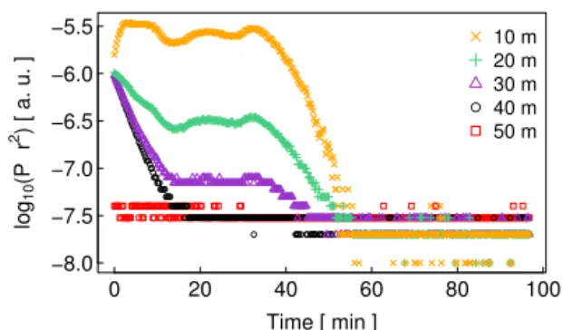
To evaluate whether the night-time climatology is a suit-able basis to assess the background signal profile, test mea-surements for four LUMO sensors with recent firmware and hardware configurations are conducted (Fig. 3c). The ceilometer window is covered by a Vaisala termination hood to mimic full atmospheric attenuation (i.e. only little signal is backscattered to the receiver which is below the sensitiv-ity of the detector). The recorded signal should represent in-ternal contributions (e.g. background signal) only. To elim-inate transient behaviour in the lowest range gates the hood measurements are taken for 30 min periods. Later tests indi-cate observations at range < 50 m may require about 1 h to settle to a characteristic value (Fig. 4), which is in agree-ment with CeiLinEx CL51 ceilometer termination hood mea-surements (Frank Wagner, DWD, personal communication, 2015; http://www.ceilinex2015.de). While variations above this range do not show a temporal drift, it is assumed that values in the first four range gates in the initial termination hood profiles are significantly overestimated. Here, the pro-file is therefore set to be constant below the fifth range gate (Fig. 3c–e).
Average termination hood profiles are compared to night-time climatology profiles from the same laser heat sink tem-perature classes. For most sensors and firmware, the me-dian night-time climatology agrees very well with the pro-file observed by the termination hood measurement (Fig. 3c). Only for ceilometer A (firmware 1.71) does the termina-tion hood measurement have a slightly different shape, al-beit with a similar order of magnitude. As there are no data available from the climatology approach for ranges below 2400 m, profiles are assumed to be constant up to this range. While this results in an obvious discrepancy between the climatology-derived background and the termination hood profiles (Fig. 3c), implications of this assumption are greatly reduced after range correction is performed (Fig. 3d–e). Al-though uncertainties remain regarding the profiles of back-ground signal below a range of 2400 m, termination hood reference measurements give confidence that the night-time climatology measurements are not significantly influenced by backscatter from atmospheric particles and hence provide reasonable estimates of the background signal. This finding is extremely useful as it allows for the background signal of
0 20 40 60 80 100
−8.0 −7.5 −7.0 −6.5 −6.0 −5.5 log 10 (P r
2 ) [ a. u. ] ● ●●●●●●●●●●●●●●●●●●●●●●●●●●●●●●●●●●●● ●●● ● ●● ●●●●● ●●●●● ●●●●●●●●●●●● ● ● ●● ●●●●●●●●●●●●●●●●●●●●●●●●●●●●●●●●●●●●●●●●●●●●●●●●●●●●●●●●●●●●● ● ●●●●●●●●●●●●●●●●●●●●●●●●●●●●●●●●●●●●●● ● ●●● ● ● ●●●● ● ● ● ● ●●●●●● ●● ● ●●● ● ●● ● ●● ● ● ● ●●● ● ●●● ●●● ● ● ● ●●●●●●●●●●●●● ●●●● ● ● ● ● ● ● ● ●●●●●● ● ●● ● ●●●●● ● ●● ● ●● ●●●● ● ●●●●●●●●●● ●●● ● ● ● ● ● ● ● ● ●●● ●● ● ● ● ● ●●● ●● ●●● ●● ● ● ● ●●●●●● ●● ● ● ● ●●●● ● ● ● ● ● ●●●●●●●●● ● ●●●●●●●●●●●●●● ● ● ●●●●● ●● ●●●●●● ● ●●●●●● ● ● ●●●●●●●● ● ● ● 10 m 20 m 30 m 40 m 50 m
Time [ min ]
Figure 4. Logarithm of range-corrected signal reported RCS=
P·r2in the first five range gates during a termination hood
mea-surement of LUMO sensor A with firmware 1.72.
ceilometer sites that were operated in the past or that are dif-ficult to access (e.g. termination hood measurements are un-feasible) to be evaluated based on the observed profile data alone.
Vaisala states (firmware release note) that no deliberate cosmetic shift is implemented in versions 1.72 and 2.03. Given that background signals from the earlier release ver-sions are much closer to 0 or even positive, it can be con-cluded that there is no (or negligible) cosmetic shift in ver-sions 1.56, 1.61, 2.01, and 2.02 and the complete back-ground signalPbg(r)is only composed of the instrument-related background signalPbgi(r). Of the versions tested, only firmware 1.71 profiles are shifted significantly to-wards negative values. The long-term estimates of hardware-and firmware-specific background signalPnightbg (instrument-related effects plus cosmetic shift; Fig. 3a) are used to deter-mine an appropriate background correction:
Pnightbg (r)=hPbgi(r)+Pcs(r)i
night. (2)
For firmware with no significant cosmetic shift, the atmo-spheric contribution to the background correction is negligi-ble so that a static correction over time can be applied defined by the night-time profiles:
the atmospheric background signal is not available for post-processing use. However, it can be approximated by the aver-age signalPtop(t )across the top range gates where the con-tributions from aerosol scattering to the signal can be deemed negligible. The calculation of Ptop(t )follows the approach taken to estimate the noise-floorF (t )(i.e. cirrus clouds are masked out; Sect. 4.2). Only for data affected by the cosmetic shift (i.e. firmware 1.71) doesPtop(t )show significant values with a clear diurnal pattern that define the temporal variations of the background while the night-time background profiles (Eq. 2) determine its range dependence. To ensure the back-ground correction Pbg(r)remains close to the climatology Pnightbg (r)when solar radiation is absent, a nocturnal average Pnighttop (mean Ptop(t )of 4 h around midnight calculated for each day to be corrected) is subtracted:
Pbg(t, r)=Pnightbg (r)−Ptop(t )−Pnighttop . (4) The derived background correctionPbg(r)(according to Eq. (4) for firmware 1.71 and Eq. (3) for other versions tested) can be applied in the post-processing to estimate the entirely background-corrected signal Pˆ without effects of
cosmetic shift from the data recorded (Eq. 1). This correc-tion reduces the range dependence of the observed signal so that the range histograms of Pˆ·r2(Fig. 1c) are more sym-metric around 0 than those ofP·r2(i.e. RCS, Fig. 1b) in all range gates in the free atmosphere; i.e. the median profile is close to 0.
All ceilometers tested here have a non-zero background profile, which confirms analysis by the Met Office (termi-nation hood measurements and case study analysis) giving a negative background for other CL31 sensors in their net-work (Mariana Adam, Met Office, personal communication, 2014–2015). This creates additional challenges when deriv-ing the aerosol backscatter coefficient from such measure-ments (Mariana Adam, Met Office, personal communica-tion, 2015). For firmware versions without (or negligible) cosmetic shift, the background signal consists solely of the instrument-related contributions which may be small. Impli-cations of these instrument-specific variations might be lim-ited for observations within clouds or in the ABL, where backscatter values tend to be large and mostly positive. How-ever, the instrument-related background signal can reach sig-nificant values that may dominate any signal differences ex-pected at the top of the ABL. The cosmetic shift in version 1.71 clearly affects observations within the ABL (Sect. 4.2). Note that the cosmetic shift and instrument-related back-ground signal should be carefully evaluated before using noise for quality-control purposes, including absolute cali-bration and SNR calculations (Sect. 4).
3.2 Range correction
For a given concentration of atmospheric scatterers (cloud, aerosol, molecules), the strength of the backscattered signal
returned to the ceilometer telescope and detector decreases by the square of the ranger. Therefore, to relate scattering coefficients at different ranges, the signalP is multiplied by r2at each range gate to obtain the RCS:
RCS(r)=P (r)·r2. (5)
The signalP is determined from the RCS reported by the CL31 by reverting Eq. (5). Vaisala instruments have an op-tion for the range correcop-tion to be applied only to the sig-nal in the lower part of the profile up to a set range rH2, where it is implicitly assumed that most of the data at further ranges consists of noise (setting: “Message profile noise_h2 off”). If no clouds are present in the profile, the raw signal is multiplied by a constant, range-invariant scale factorkH2 above rH2 (CL31: rH2=2400 m and kH2=rH22 =24002). The partly range-corrected signal reported RCSH2 has two segments:
RCSH2=
P (r)·kH2, r > rH2,
P (r)·r2, r≤rH2. (6)
When clouds are detected, the cloud signal is range-corrected using Eq. (5) for range gates where cloud is deter-mined to exist. To create a fully range-corrected signal from such observations for the whole vertical profile (according to Eq. (5), i.e. as if run with the setting “Message profile noise_h2 on”) in the absence of clouds, the scale factor needs to be reversed and the range correction applied to the obser-vations aboverH2:
RCS=
RCSH2(r)·k−H21·r2, r > rH2,
RCSH2(r) , r≤rH2. (7)
Still, this correction may only be applied where no clouds are present. Hence attenuated backscatter observations obtained with the setting “Message profile noise_h2 off” are of lim-ited use (Mariana Adam, Met Office, personal communica-tion, 2014; http://www.ceilinex2015.de). For ceilometers op-erating with “Message profile noise_h2 on”, all firmware ap-plies the range correction throughout the entire profile and no constant scale factor is incorporated in this processing step. Hence it is recommended to operate with this setting turned on.
The range histograms of the range-corrected signal (Fig. 1b, c) illustrate the increase in signal variability with range. After applying the full range correction (Eq. 7) to observations from a CL31 operated with “Message profile noise_h2 off” (rightmost panel in Fig. 1), the variability of the signal is height-invariant above the ABL (Fig. 1a), while the expected increase is found in the range-corrected sig-nal (Fig. 1b, c); i.e. it has the same signature as if it were recorded with the setting switched on.
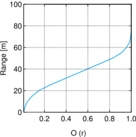
3.3 Optical overlap
in-strument. This overlap depends on instrument design. Over-lap correction functions can be applied to partly account for this effect, with dimensionless multiplication factors deter-mined empirically (e.g. Campbell et al., 2002). The over-lap correction may either be performed by firmware or dur-ing post-processdur-ing. Uncertainty remains for observations at the closest range gates (e.g. Vande Hey, 2014; Hervo et al., 2016).
Applying an optical overlap correctionO(r)to the signal, yields the overlap-corrected signal:
POC(r)=P (r)·O(r)−1. (8)
Vaisala ceilometers have a single-lens, coaxial beam setup (Münkel et al., 2009). For the CL31, complete optical overlap is reached at about 70 m from the instrument (Fig. 5) and an overlap correction is performed by the firmware (i.e.P (r)=
POC(r)). No other commercially available ceilometer offers complete overlap that close to the instrument. Vaisala over-lap functions are verified both by ray tracing simulations and laboratory measurements.
3.4 Near-range correction
Although Vaisala suggests that the attenuated backscatter profile is reliable down to the first range gate, Sokół et al. (2014) document a distinct local minimum in CL31 atten-uated backscatter observations at the fourth range gate per-sisting throughout their whole observational campaign. As others have found artefacts in CL31 profiles below 70 m (e.g Martucci et al., 2010; Tsaknakis et al., 2011), these lowest layers are often excluded during processing. As noted, van der Kamp (2008) smoothed out systematic features by strong vertical averaging, but this removes the possibility of identi-fying any atmospheric features close to the surface. With-out correction, these artefacts may cause detection of signif-icant gradients when examining profiles to diagnose mixing heights or top of the ABL. Artefacts in the first 70 m could be related to the incomplete optical overlap (Sect. 3.3) but are more likely associated with a hardware-related perturba-tion and a correcperturba-tion introduced by Vaisala to prevent unre-alistically high values in the near range when the window is obstructed.
Given the primary function of cloud base height detection, Vaisala CL31 firmware addresses effects causing extremely high backscatter values outside of clouds. Under severe win-dow obstruction (e.g. leaf on winwin-dow), values in the first range gates can be unrealistically high. A correction is ap-plied to restrict the backscatter profile in the ranges closest to the instrument. At times, this correction introduces ex-tremely small values at ranges < 50 m that are clearly offset from the observations above this height. In addition to this artefact from the obstruction correction, for some sensors, backscatter values in the range of 50–80 m are slightly off-set by a hardware-related perturbation. Both artefacts from the obstruction correction and hardware-related perturbation
0.2 0.4 0.6 0.8 1.0 0
20 40 60 80 100
O (r)
Range [m]
Figure 5.Manufacturer-deduced overlap function of Vaisala CL31
ceilometers using firmware versions 1.71, 1.72, 2.02, or 2.03 (older versions used an overlap function with 5 to 10 % lower overlap val-ues). The function, applied in the lowest range gates above the in-strument, is derived from laboratory measurements and field ob-servations under homogeneous atmospheric conditions. During the production process, the applicability of the overlap function is veri-fied for each unit. Due to the stable instrument conditions (e.g. low internal temperature variations), Vaisala expects no systematic vari-ations of the overlap function. The error is stated to be below 10 %.
do not impact cloud detection, vertical visibility, or boundary layer structures (> 80 m). It is only for attenuated backscat-ter closer than 90 m that these artefacts need to be accounted for. The issues are not firmware specific apart from versions 1.72 and 2.03, in which the artefacts of obstruction correc-tion and hardwarelated perturbacorrec-tion have been mostly re-moved. These near-range artefacts are expected to be consis-tent in time for data collected with older firmware.
0.6 1.0 1.4
RCS/RCS(10) 40
80
Range [ m ]
(a) A (403362) B (371695)
C (359787) D (387156)
0.6 1.0 1.4
RCS/RCS(10)
(b) A (91%) B (91%)
C (84%) D (88%)
0.6 1.0 1.4
RCS/RCS(10)
(c) A (9%) B (9%)
C (16%) D (12%)
0.6 1.0 1.4
RCS/RCS(10)
(d) A (296688) B (323590)
C (635741) D (641949)
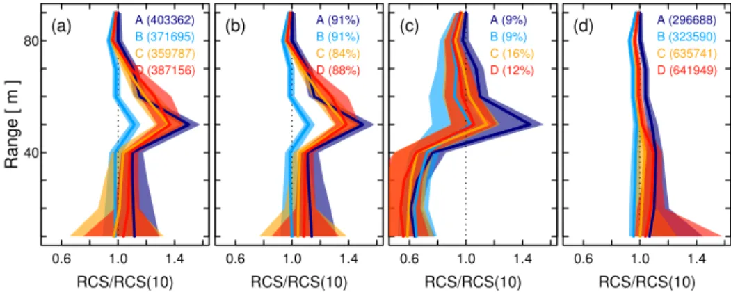
Figure 6.Median range-corrected signal reported RCS=P·r2of the lowest nine range gates (10–90 m) normalised by the value at the 10th
range gate for four LUMO sensors (Table 2) with firmware versions(a–c)1.61 (A, B) or 2.01 (C, D) in 2013 and(d)1.72 (A, B) or 2.03 (C,
D) in 2015–2016, respectively. Statistics calculated for all profiles observed between 11:00 and 16:00 UTC with RCS < 200×10−8a. u. in
the lowest 400 m: median (solid line) and interquartile rage (shading). Panels(b)and(c)separate the profiles from panel(a)into(b)profiles
with the ratio at the third range gate, i.e.|RCS(3)/RCS(10)|exceeding or equal to 0.8, while(c)shows the profiles with the same ratio less
than 0.8. For(a, d)the total number of 15 s profiles selected is indicated by sensor ID (A, B, C, or D) and in(b, c)the percentages of the
values from the total number of profiles in panel(a)are given.
indicates an overestimation of about 40–50 %, while sys-tematic differences are commonly < 20 % for the remaining range gates below 100 m. For dry and well-mixed conditions, profiles observed with firmware 1.72 or 2.03 (Fig. 6d) indi-cate that the obstruction correction and hardware-related per-turbation might be removed with these updates.
Based on the median climatological profiles (Fig. 6), a near-range correction is proposed to reduce the impact of the obstruction correction and hardware-related perturbation. Only profiles that roughly match the general shape of the cli-matology are corrected; i.e. if strong vertical gradients in the signal are observed (e.g. descending fog) the near-range cor-rection is inapplicable. However, these near-range artefacts are usually small compared to the physical processes influ-encing the attenuated backscatter across the profile.
Given that all sensors tested have a distinct peak at a cer-tain range gate (Fig. 6a) this peak is used to indicate whether a correction should be applied. The inverse approach could correct observations with a strong local minimum at the fourth range gate as reported by Sokół et al. (2014). The aim is to apply the near-range correction only to profiles with a pronounced peak value that appears physically unreason-able. First, the range gate with the peak is identified from the climatology (fifth range gate for LUMO sensors). Sec-ond, the peak strength is defined as the ratio of the range-corrected signal reported at this range gate to that reported at the adjacent gates (i.e. fourth and sixth for LUMO sen-sors). If both these peak-strength indicators of a given profile are at least 25 % as strong as the peak-strength indicators of the climatology profile, the values of this profile in the near range (< 100 m) are divided by the median climatology pro-file (Fig. 6b). Propro-files affected by the obstruction correction, i.e. with clearly offset values in the first four range gates, are treated separately. If the first peak-strength indicator (i.e. the
one below the peak) is at least 50 % as strong as the respec-tive indicator of the climatology of this regime (Fig. 6c) and the value at the range gate of the peak is greater than the values in the two range gates above, the respective median climatology profile is used for the correction (Fig. 6c).
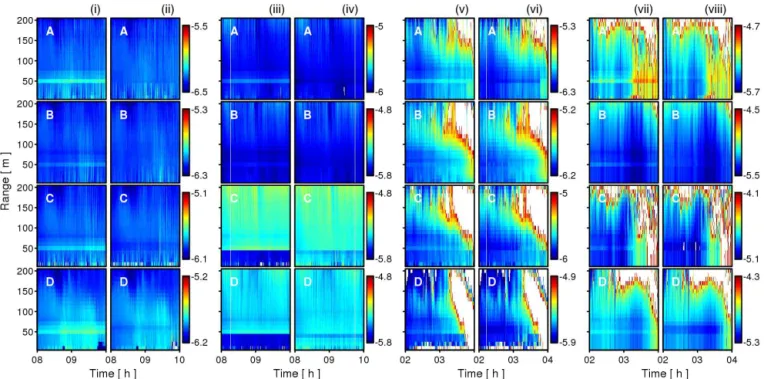
Correction functions can help to reduce the processing artefact due to the obstruction correction and the hardware-related offset as demonstrated for several case studies (Fig. 7; LUMO ceilometers A–D, see Table 2). Observations taken with firmware versions < 1.72 (for systems running with en-gine board plus receiver combination CLE311+CLR311)
or < 2.03 (CLE321+CLR321) have clear near-range effects (Fig. 6a-c) evident in the data recorded (Fig. 7i, iii, v). Two examples are clearly affected by the obstruction correction (Fig. 7iii, ceilometers C and D) with values in the lowest four range gates negatively offset. After the near-range correction is applied, this effect is reduced and the artificial peaks at the fifth range gate are mostly removed (Fig. 7ii, iv, vi). Al-though some residual effects may remain, extreme vertical gradients encountered within the lowest 100 m of the origi-nal range-corrected sigorigi-nal reported by the CL31 ceilometers are mostly removed.
Figure 7.Observations from four Vaisala CL31 ceilometers from the LUMO network (Table 2) over the first 200 m range: (i, iii, v, vii) logarithm of the range-corrected signal reported RCS (a. u.); (ii, iv, vi, viii) as in (i, iii, v, vii) but after application of correction for near-range artefacts associated with the obstruction correction and a hardware-related perturbation (see Fig. 6). Sensors were operating with firmware 1.61 (A, B) and 2.01 (C, D) on (i, ii) 10 January 2014, (iii, iv) 15 January 2014, (v, vi) 6 January 2013, and firmware 1.72 and 2.03 on (vii, viii) 13 March 2016. White areas indicate values outside of the range of values selected (see colour legends). Note that data are not absolutely calibrated.
profiles (Fig. 6). Given that the near-range correction intro-duced by Vaisala in versions 1.72 and 2.03 is not sufficient in moist conditions with gradients along the profile (Fig. 7vii), it was proposed to Vaisala to remove their correction again so that the near-range correction can be applied during post-processing.
4 Absolute backscatter and quality assurance 4.1 Absolute calibration
The range-corrected attenuated backscatter β·r2 describes the range-corrected and background-corrected signal cali-brated by the lidar constantC:
β·r2= ˆP·C−1·r2. (9)
The lidar constantCis a function of the range-independent parameters of the lidar equation, including the speed of light, area of the receiver telescope, temporal length of a laser pulse, a system efficiency term, and mean laser power per pulse (Weitkamp, 2005). It depends on instrument receiver design and its laser. When the instrument is new, system effi-ciency and laser power are high. At this stage, the lidar con-stant for internal calibration is determined by a factory-based test (C=Cfactory). Even with regular cleaning and mainte-nance, the performance of a sensor changes over time (e.g.
aging of the laser, changes in window transmissivity). To ac-count for such possible variations in laser output and detec-tor capability over time, the ceilometer firmware monidetec-tors the laser output energy and determines a relative calibration-correction factor cmonitor(t ), which is a time-specific lidar constant applied internally:
tech-nique is applied externally, i.e. as part of the post-processing:
β·r2=Pinternal·Cinternal(t )−1·cabsolute(t )−1·r2. (11) The absolute calibration coefficientcabsolute(t )may be con-stant in timecabsolute(t )=cabsolute (Hopkin et al., 2016). A laser at the CL31 operating wavelength (≈905 nm) is
sensi-tive to absorption of water vapour in the atmosphere, which can have implications for the absolute calibration (Markow-icz et al., 2008; Wiegner and Gasteiger, 2015). As evaluation of absolute calibration techniques is beyond the scope of this study, for simplicity the impact of this external calibration is neglected (i.e.cabsolute(t )=1).
4.2 Signal strength and noise
Given that noise is a critical component of the attenuated backscatter recorded, data with values below a certain SNR are unlikely to contain sufficient information about the state of the atmosphere. Where high-resolution observations are obtained, rolling spatial (along-range) and temporal averag-ing increases the signal contribution relative to the noise. For every range gater and time stept, the smoothed attenuated backscatter is the average over a temporal window of fixed size 2 wt+1 (with wt time steps) and a range window of fixed size 2wr+1:
βsmooth(t, r)=(2wt+1)−1·(2wr+1)−1 (12)
Xk=r+wr
k=r−wr
Xh=t+wt
h=t−wtβ ( h, k) .
Optimal window length depends on hardware characteris-tics (i.e. noise levels), resolution settings for raw data ac-quisition, and the application. Here, window lengths com-bining to a total of about 1000 have been found suitable to prepare data for the detection of mixing height with a relatively larger temporal averaging window (i.e. wt=50; wr=5, which equals 25.25 min and 110 m for the LUMO sensors; see Table 2) as features of the ABL structure show more variability in the vertical than over time. Such large window sizes can significantly improve the SNR, i.e. signal strength compared to average background noise, while small-scale variability is mostly preserved due to the moving aver-age. If block averaging is applied, shorter averaging windows might be more appropriate. For example, Sokół et al. (2014) find a 5 min window suitable for block averaging attenuated backscatter of a CL31 prior to mixing height analysis in the morning transition period as boundary layer dynamics may vary at 30–60 min timescales. To significantly increase SNR, Stachlewska et al. (2012) use Gaussian smoothing (Jenoptik CHM15K ceilometer) with linearly increasing range window widths; however, this is can result in extensive computing time. BLview (Vaisala’s boundary layer detection software, e.g. used by Tang et al., 2016) has range-variant smoothing windows.
The quality of range-corrected attenuated backscatter can be evaluated by comparison to the noise floor. The latter rep-resents variations associated with electronic and optical noise and noise introduced by the solar background light. If no high cirrus clouds are present, it is assumed the signal from the very highest range gates contains only noise (i.e. atmospheric signal contribution is negligible). In this case, the noise floor F can be defined as the meanβ plus standard deviationσβ of the attenuated backscatterβ (i.e. before range correction) across a certain number of gates from the top of the profile. Statistics are applied across these gates at the top of the pro-file and moving temporal windows (as in Eq. 12):
F (t )=β (t )+σβ(t ) . (13)
Here, the highest 300 m of the profile (N=30 at 10 m resolu-tion) are used to determine the noise floor to ensure sufficient representation of the range variability. Similar results are ob-tained with slightly more range gates. The discontinuity and increased noise levels around 7000 m (Sect. 3.1) make it in-advisable to include more than 600 m to calculate the noise floor. The meanβacross the top range gates is usually small and fluctuates around 0. However, if the background correc-tion (Sect. 3.1) is not performed it can have a slight offset from 0 and even a diurnal pattern for data acquired with firmware version 1.71, which performs the cosmetic shift based on the dynamic zero-bias level (Sect. 2). Calculated from the entirely background-corrected signal or attenuated backscatter (see Eq. 1–4), the noise floorF is nearly equal to the standard deviationσβ across the top range gates.
To ensure that profiles used for the calculation ofF do not contain any cirrus clouds, which can provide significant backscatter even at the furthest ranges of the profile, the “rel-ative variance” RV(t, r)(or coefficient of variation) is used to mask cloud observations (Manninen et al., 2016). For each timetand ranger(at the top of the profile), the relative vari-ance is the ratio of the standard deviationσβ(t, r)to the mean β(t, r), with statistics applied over moving windows (as in Eq. 12), along range and time (here,wr=wt=3 were used):
RV(t, r)=
σ
β(t, r)
β (t, r)
2
. (14)
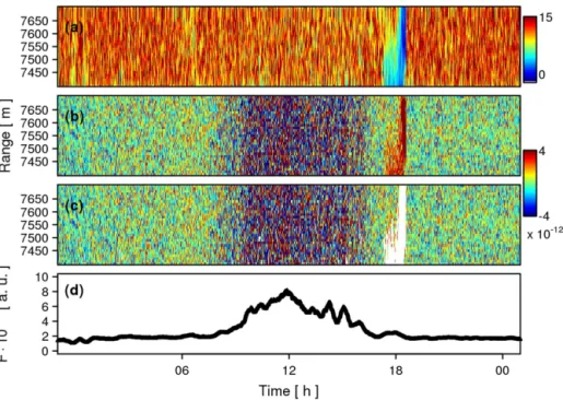
Figure 8.Observations from Vaisala CL31 sensor D (Table 2) at top range gates (7410–7700 m) with cirrus during the early evening on
1 February 2013:(a)relative variance RV (Eq. 14);(b)background-corrected signalPˆ;(c)same as(b)but only including observations with
RV > 1; and(d)time series of the noise floorF(Eq. 13) based on the cleaned signal shown in(c)with missing values interpolated linearly.
● ● ● ● ●●●●●●●● ● ●●● ● ● ● ● ● ● ● ● ● ● ● ● ● ● ●●● ●●●●●●●●●●●●●●●●●●●●●●●●●●●●●●●●●●●●●●●●●●●●●●●●●●●●●●●●●●●●●●●●●●●●●●●●●●●●●●●●●●●●●●●●●●●●●●●●●●●●●●●●●●●●●●●●●●●●●●●●●●●●●●●●●●●●●●●●●●●●●●●●●●●●●●●●●●●●●●●●●●●●●●●●●●●●●●●●●●●●●
−0.50 0.0 0.5 1.0 1.5 2.0 20 40 60 80 100 SNR Acceptance [%] ● ● ● ● ●●● ●●● ●● ● ●● ● ● ● ● ● ● ● ● ● ● ● ● ● ● ● ● ● ● ●● ●●●●●●●●●●●●●●●●●●●●●●●●●●●●●●●●●●●●●● ● ●●●●●●●●●●●●●●●●●●●●●●●●●●●●●●●●●●●●●●●●●●●●●●●●●●●●●●●●●●●●●●●●●●●●●●●●●●●●●●●●●●●●●●●●●●●●●●● ●●●●●●●●●●●●●●●●●●●●●●●●●●●●●●●●●●●●●●●●●●●●● ● ● ● ● ● ●●●●●●●●● ● ● ● ● ● ● ● ● ● ● ● ● ● ● ● ●● ● ● ●●●●●●●●●●●●●●●●●●●●●●●●●●●●●●●●●●●●●●●●●●●●●●●●●●●●●●●●●●●●●●●●●●●●●●●●●●●●●●●●●●●●●●●●●●●●●●●●●●●●●●● ●●●●●●●●●●●●●●●● ●●●●●●●● ● ●●●●●●●●●●●●●●●●●●●●●●●●●●●●●●●●●●●●●● ●●●●●●●●●● ● ●●● ● ●●●●●● ● ● ●● ● ●● ● ●●●●●●●●● ●● ● ●● ● ●●●● ● ● ● ● ● ● ● ● ● ● ● ● ● ● ● ● ● ● ● ●● ●● ● ●●●●●●●●●●●●●●●●●●●●●●●●●●●●●●●●●●●●●●●●● ● ●● ● ●●●●●●●●●●●●●●●●●●●●●●●●●●●●●●●●●●●●●●●●●●●●●●●●●●●●●●●●●●●●●●●●●●●●●●●●●● ●●●●●●●●●●●●●●●●● ● ●● ● ●●●●●●●●●●●●●●●●●●●●●●●●●●●●●●●●●●●●●●● ● ● ● ● ●● ● ●●●●●●●●● ● ●● ● ● ● ● ● ● ● ● ● ● ● ● ● ● ● ● ● ●● ● ●●●●●●●●●●●●●●●●●●●●●●●●●●●●●●●●●●●●●●●●●●●●●●●●●●●●●●●●●●●●●●●●●●●●●●●●●●●●●●●●●●●●●●●●●●●●●● ●●●●●●●●● ●●● ●●●●●●●●● ●●●●●●●●● ●●●●●● ●●●●●●●●●●●●●●●●●●● ●●●●●●●● ●●●● ●●●●●●●●●●●●●●●●●●●●●●● ● ● ● ● 1.61 1.71 1.72 2.03 50 % 90 %
Figure 9.Acceptance (%) based on Welch’sttest with apvalue of 0.01 of smoothed, not range-corrected, attenuated backscatter (Eq. 12) to be significantly higher than the noise floor (Eq. 13), binned by the corresponding signal-to-noise ratio (SNR, Eq. 15) for four selected cases (24 h each; range 50–3000 m shown for sim-plicity) of observations taken with different firmware versions (see legend). The shaded area marks the SNR region corresponding to acceptance levels of 50–90 %.
convert the RV field (Fig. 8a) into a mask to remove the cir-rus signal from the attenuated backscatter (Fig. 8b). Based on the attenuated backscatter with clouds masked out (Fig. 8c), the noise floor F is calculated over the course of the day (Fig. 8d) and the area missing due to the presence of cirrus is interpolated linearly over the time period where the atten-uated backscatter has been masked out.
The SNR is calculated from smoothed, non-range-corrected attenuated backscatter (Eq. 12) and the noise floor F:
SNR(t, r)=βsmooth(t, r)
F (t ) . (15)
Figure 10.CL31 observations on 24 July 2012 (rows 1 and 2), 22 June 2014 (rows 3 and 4), and 29 June 2016 (row 5) from four sensors with
firmware version in brackets: A (1.61), B (1.71), C (2.02), and S (2.01); see Table 2.(a)Range-corrected attenuated backscatterβ·r2at 15 s
resolution (rows 1–4) and 30 s (row 5) as reported;(b)as in(a)with running average (∼25 min,∼100 m) applied (Eq. 12);(c)as in(b)but
including correction of instrument-related background signal and potential cosmetic shift (see Sect. 3.1); and(d)as in(c)but filtered for
SNR >T2, withT2=0.18 (see discussion on Fig. 9). Note: for simplicity the absolute calibration constant is here assumed to becabsolute=1
(Sect. 4.1) for all sensors. This is not necessarily expected to be a correct assumption in reality but applied to show the impact of corrections on the final product, i.e. the attenuated backscatter.
by the fact that most observations with no significant sig-nal contribution become or remain negative after smoothing (Eq. 12) has been applied. If attenuated backscatter profiles are used for the detection of layers in the ABL, it is recom-mended to include data with βsmooth (SNR >T2)at a given point in time and rangerbut also if the threshold is exceeded at a certain range below (r−1r). This is to ensure gradients
can be calculated in the entrainment zone even if the clear air above the ABL is associated with very low SNR values. The appropriate range distance1rdepends on the degree of smoothing applied and the calculation of the vertical gradient for layer detection.
firmware versions is illustrated based on three case study days (Fig. 10): 24 July 2012 with clear-sky conditions com-paring sensor A running with firmware version 1.61 (row 1) and to sensor C with firmware 2.02 (row 2), 22 June 2012 with some boundary layer clouds present comparing sen-sor B with 1.71 (row 3) and sensen-sor C with firmware 2.02 (row 4), and 29 June 2015 with a few isolated medium- and high-level clouds showing observations from sensor S with 2.01 (row 5). The range-corrected attenuated backscatter re-ported (Fig. 10a) is quite noisy in all sensor observations and the evolution of the ABL is difficult to discern. When the moving average is applied (Fig. 10b), the signal contribu-tion clearly increases so that aerosol layers can be identified visually. However, the contrast between ABL and the clear air above varies greatly with sensor and firmware version. While the ABL reveals distinct attenuated backscatter signa-tures for data from sensor C with firmware 2.02 (rows 2 and 4), the values in the free troposphere are elevated for sen-sors A (row 1) and S (row 5). This is explained by the dif-ferent profiles of background signal inherent in these obser-vations (Fig. 3a): sensor C has a small and slightly negative background signal which barely affects observations above the ABL, while both sensor A (firmware 1.61) and sensor S (2.01) have a positive background signal leading to an over-estimation of signal below about 5000 m. Even more severe is the impact of the cosmetic shift inherent in observations from sensor B (1.71; row 3), which reduces the signal signifi-cantly even within the ABL. For the example shown, average values become negative below the boundary layer clouds so that no mixing height detection algorithm would be able to derive relevant statistics.
The described artefacts can mostly be accounted for by the proposed background correction (Eq. 1–4; Fig. 10c). While it can help to improve the contrast at the boundary layer top for sensors A (row 1) and S (row 5), it can revert the cos-metic shift in data from sensor B (row 3). In the latter case, the background correction can increase data availability. It should be noted that the systematic ripple effect (sensors B and C; see Sect. 3.1) becomes apparent after the back-ground correction. Although the ripple is somewhat coher-ent and not truly random, affected areas above the ABL can still be successfully masked by the SNR filter (Fig. 10d). For all sensors, the statistical threshold helps to distinguish data with significant information content (compare Fig. 10c, d) so that quality can be assured for later applications (e.g. mixing height detection). Still, some significant noise may remain near the ABL top for the older generation of hardware run-ning with firmware 1.xx (row 1 and 3). It can be concluded that data quality of sensors of the recent hardware genera-tion, i.e. those operating firmware version 2.xx (here sensors C and S) are clearly superior to older generations (sensors A and B).
5 Summary
Ceilometers are valuable instruments with which to study not only clouds but also the ABL and elevated layers of aerosols. Vaisala CL31 sensors provide good-quality atten-uated backscatter. While their cloud base height product might be readily useful, to understand the profiles of atten-uated backscatter the user needs to be aware of the instru-ment model’s specific hardware and firmware. The following sections summarise aspects useful to consider in the post-processing of CL31 ceilometer attenuated backscatter pro-files.
By taking into account these instrument-specific aspects of the CL31 profile observations, data quality and availabil-ity can be improved. If data are collected according to best practice, as recommended (Sect. 5.3), issues are being cor-rected for in the post-processing (e.g. applying the proposed methods) and sensors are carefully calibrated, then the atten-uated backscatter observations might prove useful for NWP model verification and evaluation, and potentially even for data assimilation.
5.1 Instrument-specific characteristics and issues Initial internal averaging of the sampled ceilometer signal is applied over selected time intervals that depend on the range and the user-defined reporting interval for firmware versions < 1.72, 2.01, and 2.02. Data acquired with firmware 1.72 or 2.03 are more consistent than earlier versions because the whole profile (at all range gates) is treated equally with an internal averaging interval of 30 s.
If the user-defined reporting interval is shorter than 30 s, consecutive profiles partly overlap in time and are hence not completely independent.
When averaging several profiles, a discontinuity is evident at around both 4940 and 7000 m for all sensors and firmware versions. These regions of increased noise are introduced by the data storage procedure of the firmware, which slightly changes its operating mode after a certain number of gates have been collected. Care should be taken when looking at gradients or statistics near these ranges.
Depending on firmware version, a “cosmetic shift” is ap-plied to the attenuated backscatter profiles. This shift should be reversed before using any part of the profile for analy-sis. Of the firmware tested, the cosmetic shift appears to be negligible for all versions except for 1.71, in which a strong negative shift is applied to the observations.