www.biogeosciences.net/10/1561/2013/ doi:10.5194/bg-10-1561-2013
© Author(s) 2013. CC Attribution 3.0 License.
Biogeosciences
Geoscientiic
Geoscientiic
Geoscientiic
Geoscientiic
Simulating the vegetation response in western Europe to abrupt
climate changes under glacial background conditions
M.-N. Woillez1, M. Kageyama1, N. Combourieu-Nebout1, and G. Krinner2
1LSCE/IPSL INSU, CEA-CNRS-UVSQ UMR8212, CE Saclay, l’Orme des Merisiers, 91191 Gif-sur-Yvette Cedex, France 2LGGE, CNRS UMR5183, 54 rue Moli`ere, 38402 St. Martin d’H`eres Cedex, France
Correspondence to:M.-N. Woillez ([email protected])
Received: 9 August 2012 – Published in Biogeosciences Discuss.: 19 September 2012 Revised: 21 December 2012 – Accepted: 31 January 2013 – Published: 7 March 2013
Abstract. The last glacial period has been punctuated by two types of abrupt climatic events, the Dansgaard–Oeschger (DO) and Heinrich (HE) events. These events, recorded in Greenland ice and in marine sediments, involved changes in the Atlantic Meridional Overturning Circulation (AMOC) and led to major changes in the terrestrial biosphere.
Here we use the dynamical global vegetation model OR-CHIDEE to simulate the response of vegetation to abrupt changes in the AMOC strength. We force ORCHIDEE of-fline with outputs from the IPSL CM4 general circulation model, in which the AMOC is forced to change by adding freshwater fluxes in the North Atlantic. We investigate the impact of a collapse and recovery of the AMOC, at differ-ent rates, and focus on Western Europe, where many pollen records are available for comparison.
The impact of an AMOC collapse on the European mean temperatures and precipitations simulated by the GCM is rel-atively small but sufficient to drive an important regression of forests and expansion of grasses in ORCHIDEE, in qualita-tive agreement with pollen data for an HE event. On the con-trary, a run with a rapid shift of the AMOC to a hyperactive state of 30 Sv, mimicking the warming phase of a DO event, does not exhibit a strong impact on the European vegetation compared to the glacial control state. For our model, simulat-ing the impact of an HE event thus appears easier than sim-ulating the abrupt transition towards the interstadial phase of a DO.
For both a collapse or a recovery of the AMOC, the veg-etation starts to respond to climatic changes immediately but reaches equilibrium about 200 yr after the climate equili-brates, suggesting a possible bias in the climatic reconstruc-tions based on pollen records, which assume equilibrium
be-tween climate and vegetation. However, our study does not take into account vegetation feedbacks on the atmosphere.
1 Introduction
The last glacial period (10–90 ky BP) has been punctuated by two types of abrupt climatic changes, the Dansgaard– Oeschger (DO) events (Dansgaard et al., 1993) and Heinrich events (Heinrich, 1988). The DO events are characterized by an initial abrupt warming of up to 8 to 16◦C over Greenland in a few decades (Johnsen et al., 1992, 1995; Landais et al., 2004; Wolff et al., 2010), followed by a warm phase (in-terstadial) during which the temperature gradually decreases over several hundred to several thousand years , ended by an abrupt return to cold conditions (stadial). Some of the stadi-als correspond to Heinrich events (HE), which are defined as massive iceberg discharges from the Laurentide ice sheet in the North Atlantic, occurring every 5 to 7 ky and recorded in marine sediment cores by the presence of ice-rafted detritus (Heinrich, 1988; Bond and Lotti, 1995). DO events appar-ently occurred with a periodicity of around 1500 yr (Alley et al., 2001; Schulz, 2002), however the significance of this periodicity is debated and some authors claim that the recur-rence actually cannot be distinguished from a random occur-rence (Ditlevsen et al., 2007).
reconstructions from Antarctica show smaller and more gradual fluctuations, approximately out of phase with the Greenland temperature records (Jouzel et al., 2003; Blunier et al., 1998; EPICA Community Members, 2006). Abrupt changes opposite to the North Atlantic signal are recorded in the South Atlantic, at the present-day northern margin of the Antarctic Circumpolar Current (Barker et al., 2009). This opposite behaviour of the two hemispheres, called “bipolar see-saw” (Crowley, 1992; Stocker and Johnsen, 2003), has been explained by a reduction of the northward heat trans-port when the AMOC slows down, leading to a cooling of the Northern Hemisphere and to a warming of the Southern Hemisphere. The mechanism has been confirmed by many modelling studies which successfully reproduced the bipolar see-saw pattern when the AMOC collapses (see the reviews of Clement and Peterson, 2008 and Kageyama et al., 2010).
Contrary to HE events, the shift from a stadial to an inter-stadial state during a DO event does not seem to be associ-ated with strong changes in the AMOC (Elliot et al., 2002). The modelling study by Ganopolski and Rahmstorf (2001) suggests that DO events are caused by shifts between two different modes of convection of the AMOC, driven by small fluctuations of the freshwater flux. It has been suggested that such fluctuations could be triggered by changes in solar irra-diance (Braun et al., 2005), which could impact the ablation rate of the ice sheets (Woillez et al., 2012). However, so far, the ultimate cause of DO events remains an open issue.
Pollen records from marine and terrestrial cores reveal abrupt vegetation changes around the whole North Atlantic region, that can be correlated to DO and HE events. In Florida, records from Lake Tulane show an antiphase re-lationship with the North Atlantic region: oak-scrub and prairie vegetation during interstadials and the development of pine forest during stadials (Grimm et al., 2006), indicat-ing a wetter and warmer climate for the stadials. In West-ern Europe, millennial-scale climatic variability had strong impacts on vegetation (see Fletcher et al. (2010) for a re-view). In the British Isles, north-west France, the lowlands of the Netherlands, Northern Germany, Denmark and north-west Scandinavia interstadials are characterized by open, treeless vegetation, whereas stadials are often marked by the presence of non-organic deposits indicating a very sparse or absent vegetation (Fletcher et al. (2010) and references therein). In France, the records from lacustrine deposits from La Grande Pile, Les Echets and the Velay maars (Woillard, 1978; de Beaulieu and Reille, 1984, 1992a,b; Reille and de Beaulieu, 1988, 1990) indicate that the last glacial was dominated by steppe-tundra vegetation, with some episodes of open woodland which might correspond to some DO events. The South of Italy (Allen et al., 1999), Alpine re-gions, the Bay of Biscay and Spain (Fletcher et al., 2010) also show increases in arboreal vegetation during intersta-dials. In western France, aBetula-Pinus-deciduous Quercus
forest alternates with steppic plants (S´anchez-Go˜ni et al., 2008). Several marine cores from the Atlantic or
Mediter-ranean Iberian margins (see Combourieu-Nebout et al., 2002; S´anchez-Go˜ni et al., 2002; Fletcher and S´anchez-Go˜ni, 2008; Combourieu-Nebout et al., 2009b) show an alternance of temperate forest during interstadials and steppic vegetation during stadials. The percentage of steppic plants such as
Artemisiais especially high during stadials associated to a Heinrich event (Combourieu-Nebout et al., 2002; Fletcher and S´anchez-Go˜ni, 2008; Fletcher et al., 2010). More pre-cisely, southern Iberia is occupied by Mediterranean forest (deciduous and evergreenQuercusspecies) during interstadi-als and by semi-desert vegetation withArtemisia, Chenopo-diaceaea and Ephedra during stadials, and in North-West Iberia deciduousQuercus andPinus forest alternates with grass and heathland (S´anchez-Go˜ni et al., 2008).
To our knowledge, only a few modelling studies have ad-dressed the issue of the vegetation response to abrupt climate changes. Scholze et al. (2003) performed freshwater hosing experiments with the ECHAM3 AOGCM to simulate an ide-alized analogue of the Younger Dryas and used these cli-mate forcings to run the dynamical global vegetation model (DGVM) LPJ. The strong surface cooling over the Northern Hemisphere leads to a decrease of temperate forests, replaced by boreal forests and C3 grass in northwest Europe and by C3 grass only in Southern Europe.
Kageyama et al. (2005) used the IPSL GCM and the OR-CHIDEE DGVM to investigate the impact of Heinrich event 1 (H1) on the climate and vegetation of the western Mediter-ranean Sea. The climate of H1 was simulated by lowering the SSTs by up to 4◦C over the North Atlantic compared to the control simulation for the Last Glacial Maximum (LGM). The vegetation simulated by ORCHIDEE for H1 presented a strong reduction of tree cover over France and a regression of grass both over France and over the Iberian Peninsula.
In a previous study, Woillez et al. (2011) investigated the relative impact of climate and CO2on the vegetation simu-lated by the ORCHIDEE DGVM at the LGM. The results show that low CO2 has a strong impact on tree cover re-sponse to glacial conditions.This impact depends on both the background climate and the type of vegetation. Here we want to investigate (with the same DGVM) the links be-tween glacial vegetation and the AMOC state, with a focus over Western Europe. How does the vegetation respond to AMOC changes? Can the model reproduce the changes in-ferred from pollen data for HE and DO events? Is the re-sponse synchronous with the AMOC?
We start from the glacial state of vegetation simulated by ORCHIDEE in Woillez et al. (2011) and investigate the re-sponse of vegetation to climate changes simulated by the IPSL CM4 AOGCM in response to abrupt changes in the AMOC strength. We focus on the timing of the response of vegetation compared to the timing of the AMOC evolution and analyse the specific response of the different plant func-tional types (PFTs) simulated in ORCHIDEE, in order to in-vestigate their different sensitivities to the simulated abrupt climate changes. We also analyse the relative impact of tem-perature and precipitation changes, which has not been in-vestigated in the studies cited above. Distinguishing the im-pact of temperature and precipitation might help to better constrain the temperature and precipitation changes inferred from pollen records during abrupt changes.
The layout of the paper is as follows: Sect. 2 describes the ORCHIDEE and IPSL models and the design of the differ-ent atmospheric and vegetation runs. In Sect. 3 we presdiffer-ent the climatic changes simulated by the model in response to changes in the AMOC strength and the response of vegeta-tion at the global scale. We then focus on Western Europe in Sects. 4 (climate) and 5 (vegetation), a region of special interest given the pollen records available for a model-data comparison. In the present study, we define Western Europe as the area between 32◦and 60◦N and 15◦W and 20◦E. We
discuss our results and conclude in Sect. 6.
2 Material and methods
2.1 The ORCHIDEE dynamic global vegetation model
ORCHIDEE (Krinner et al., 2005) is composed of three cou-pled submodels: the surface vegetation-atmosphere transfer
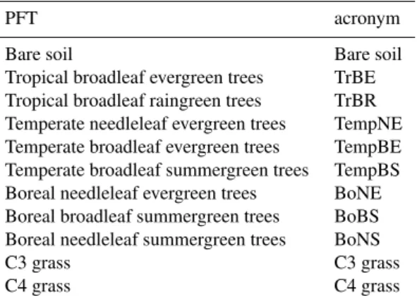
scheme SECHIBA, a module for phenology and carbon namics of the terrestrial biosphere (STOMATE), and a dy-namical vegetation model inspired from LPJ (Sitch et al., 2003). The model simulates the distribution of ten different plant functional types (PFTs) and bare soil (for the list of the PFTs and the corresponding acronyms used in this study see Table 1), which can coexist on the same grid cell, as a result of climatic forcings and competitivity between these differ-ent PFTs. The spatial resolution in the vegetation model is identical to the spatial resolution in the climate model. The dynamical part simulates competitive processes such as light competition, sapling establishment, or tree mortality. In this study, ORCHIDEE is forced “offline” by the high-frequency outputs (time step = 6 h) from the IPSL CM4 model. There is no feedback between vegetation and the atmosphere. The model requires the following variables: temperature, precip-itation, specific humidity, wind, surface pressure, shortwave and longwave radiative fluxes.
2.2 The climatic forcings computed with the IPSL CM4
GCM
The IPSL CM4 AOGCM (Marti et al., 2010) is composed of LMDz.3.3, the atmospheric general circulation model, and ORCA2, the ocean module. The resolution for the atmo-sphere is 96×72×19 in longitude×latitude×altitude and a regular horizontal grid. The ocean is simulated over an irregular horizontal grid of 182×149 points and 31 depth levels. The coupling is performed by the OASIS coupler. LMDz includes the surface vegetation model ORCHIDEE (Krinner et al., 2005), sea ice is dynamically simulated by the Louvain-La-Neuve sea Ice Model (LIM2) but glacial ice sheets are fixed. Land, land-ice, ocean and sea ice can coexist on the same grid cell of LMDz.
Four different glacial climatic simulations are performed. The LGM control run (ON ctrl) is the IPSL PMIP2 LGM run (see LGMb in Kageyama et al., 2009 for details; Bracon-not et al., 2007 and http://pmip2.lsce.ipsl.fr for the PMIP2 project). The glacial boundary conditions follow the PMIP2 protocol: ICE-5G reconstruction for the ice sheets (Peltier, 2004); CO2, CH4 and N2O levels set to 185 ppm, 350 ppb and 200 ppb respectively (Monnin et al., 2001; D¨allenbach et al., 2000; Fl¨uckiger et al., 1999), orbital parameters for 21 ky BP (Berger, 1978). Vegetation is fixed to its present-day distribution on the ice-free areas, including agriculture, since interactive dynamic vegetation is unavailable in this version of IPSL CM4.
Table 1.Plant functional types (PFT) in ORCHIDEE and acronyms used in this study.
PFT acronym
Bare soil Bare soil
Tropical broadleaf evergreen trees TrBE
Tropical broadleaf raingreen trees TrBR
Temperate needleleaf evergreen trees TempNE
Temperate broadleaf evergreen trees TempBE
Temperate broadleaf summergreen trees TempBS
Boreal needleleaf evergreen trees BoNE
Boreal broadleaf summergreen trees BoBS
Boreal needleleaf summergreen trees BoNS
C3 grass C3 grass
C4 grass C4 grass
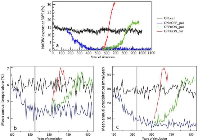
The freshwater discharge performed in ONtoOFF grad leads to a gradual collapse of the AMOC, mimicking the ef-fect of a Heinrich event. The NADW (North Atlantic Deep Water) export at 30◦S drops from about 13 Sv in ON ctrl to
0 Sv within 250 yr of simulation (Fig. 1a). Once the freshwa-ter flux is stopped, the AMOC does not recover and remains in an “off” state. This stability of the collapsed state is not a common behaviour in AOGCMs. In most of them a spon-taneous recovery of the AMOC occurs once the freshwater flux is stopped (e.g. Manabe and Stouffer, 1995; Hu et al., 2008; Otto-Bliesner and Brady, 2010).
A gradual recovery occurs in OFFtoON grad as soon as the negative freshwater flux is imposed. The NADW export reaches the initial state after 250 yr, and stabilizes at 17 Sv about 100 yr later. In OFFtoON fast, the−0.5 Sv imposed in the North Atlantic leads to a quasi instantaneous recovery of the AMOC, which is back to initial state within about 70 yr. At the end of the simulation, the NADW export is higher than 30 Sv and equilibrium has not been reached (Fig. 1a). This last simulation was designed to mimic the effect of the abrupt warming phase of a DO event. We further describe the climate changes in these runs in Sect. 3.
2.3 Experimental design of the ORCHIDEE off-line
runs
Our aim is to simulate the response of the glacial vegeta-tion to abrupt AMOC changes and to investigate whether the vegetation evolution is synchronous with the AMOC, for both a collapse and a recovery at different rates. Therefore, we use the climatic forcings from ON ctrl, ONtoOFF grad, OFFtoON grad and OFFtoON fast to design different sce-narios of AMOC changes and perform six simulations with ORCHIDEE off-line:
– ON ctrl (1000 yr): the LGM control simulation, forced with 1000 yr of the IPSL simulation ON ctrl. The simu-lation starts at the end of a spinup phase designed as fol-lows: ORCHIDEE is run during 500 yr with the ON ctrl
LGM climate, starting from bare ground. Then the soil carbon submodel is run alone for 10 000 yr, to equili-brate the carbon stocks. Finally the whole model is run for another 50 yr (simulation described in Woillez et al., 2011).
– ONtoOFF grad (800 yr): this simulation starts from the equilibrium state of ON ctrl and we test the impact of the gradual collapse of the AMOC on vegetation by forcing ORCHIDEE with the climatic forcings from the IPSL simulation ONtoOFF grad.
– ONtoOFF inst (400 yr): this simulation starts from the equilibrium state of ON ctrl and tests the impact of an instantaneous collapse of the AMOC. We impose di-rectly the climate from the last 400 yr of the IPSL sim-ulation ONtoOFF grad.
– OFFtoON grad (430 yr): the run starts at year 578 of ONtoOFF grad and we force the model with the climate from the IPSL simulation OFFtoON grad, with a grad-ual recovery of the AMOC.
– OFFtoON fast (150 yr): the run starts at year 578 of ONtoOFF grad and we force the model with the climate from the IPSL simulation OFFtoON fast and a very fast recovery of the AMOC.
– OFFtoON inst (230 yr): the run starts at year 578 of ONtoOFF grad and we force the model with the cli-mate from the IPSL simulation ON ctrl, which corre-sponds to an instantaneous recovery of the AMOC, but to a value lower than the final value of OFFtoON grad and OFFtoON fast (Fig. 1a).
Two additional simulations, starting from the equilibrium state of ON ctrl, are performed to test the relative impact of temperature and precipitation changes between ON ctrl and ONtoOFF grad
– ONtoOFF precip (428 yr): same climatic forcings as for ON ctrl except for precipitation, taken from the first 428 yr of ONtoOFF grad.
– ONtoOFF temp (428 yr): same climatic forcings as ON ctrl except for temperature, taken from the first 428 yr of ONtoOFF grad.
These runs are crude tests, since we do not take into ac-count the fact that climatic variables are not fully indepen-dent from one another, but they can nonetheless allow us to test which of these two parameters have the strongest impact on vegetation. We do not test the relative impact of changes in shortwave radiations, wind and specific humidity.
All these ORCHIDEE runs are performed with
Fig. 1. (a)Temporal evolution of the NADW export at 30◦S, in Sv.(b)Evolution of the mean annual temperature (◦C) and(c)the mean annual precipitation over Western Europe (lat = 32/60◦, lon =−15/20◦) for ON ctrl, ONtoOFF grad, OFFtoON grad and OFFtoON fast.The curves correspond to values averaged only over the land points and for successive periods of 10 yr of the simulations. The vertical grey bars indicate when the AMOC is fully collapsed in ONtoOFF grad.
3 Global response of climate and vegetation to AMOC
changes
3.1 Climate
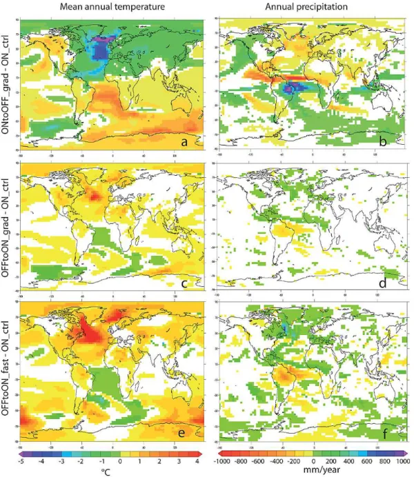
The climatic response concomitant with the AMOC collapse has already been described in detail in Kageyama et al. (2009) (comparison between LGMb (= ON ctrl) and LGMc (= ONtoOFF grad)). We briefly recall here the main features of the response in the mean annual temperature and annual precipitation. The collapse of the AMOC in ONtoOFF grad leads to a typical bipolar see-saw, with cooling of the Northern Hemisphere and warming of the Southern Hemisphere (Fig. 2a), as simulated with other models (e.g. Claussen et al., 2003; Kageyama et al., 2010) and in broad agreement with data for stadials (see the review by Voelker, 2002). The strongest temperature anomalies in ONtoOFF grad compared to ON ctrl are found over the Atlantic ocean. The mean annual surface air tem-perature at the end of ONtoOFF grad compared to ON ctrl is decreased by more than 5◦C South of Iceland, and by about 4◦C in the mid-latitude North Atlantic. The South Atlantic is warmer by 3–4◦C. The cooling over Eurasia is
limited to−1◦/−2◦C and the Pacific side of North America
even experiences a warming of about 1◦C (Fig. 2a). The precipitation response (Fig. 2b) is characterized by a strong drying over the North Atlantic and Western Europe and a southward shift of the inter-tropical convergence zone (ITCZ) over the Atlantic basin and adjacent continents, leading to a decrease of precipitation over the Sahel zone (in agreement with data, see Tjallingii et al., 2008) and the north of South America and to an increase over eastern Brazil.
At the end of OFFtoON grad, the higher AMOC strength (18 Sv, see Fig. 1a) compared to its mean strength in ON ctrl (about 13 Sv) leads to the opposite response, with a slight northward shift of the ITCZ, leading to a decrease in precipi-tation of about−100 mm yr−1over Brazil and an increase in temperature of about 3◦C in the North Atlantic (Fig. 2c, d).
The warming over the adjacent continents is limited to about 1◦C over North America and less than 1◦C over the Iberian peninsula. The temperature changes over the rest of West-ern Europe are not statistically significant and precipitation changes are small and restricted to a few grid cells.
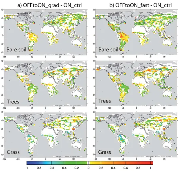
Fig. 2.L.h.s.: difference in mean annual surface temperature (◦C). R.h.s.: difference in annual precipitation (mm yr−1). Top: ONtoOFF grad– ON ctrl; middle: OFFtoON grad–ON ctrl; bottom: OFFtoON fast–ON ctrl. White areas are regions were differences are not significant at the 95 % level. ON ctrl: average over years 201–250; ONtoOFF grad: average over years 401–450; OFFtoON grad: average over the last 30 yr of the run; OFFtoON fast: average over the last 20 yr of the run.
and a strong warming occurs in the North Atlantic (Fig. 2e, f). The increase in the surface air temperature is about 6◦C at 50◦N, up to 10◦C in the Labrador Sea and about 3◦C at 70◦N. The temperature increase in the Labrador Sea is asso-ciated to an increase in precipitation of about 700 mm yr−1. This pattern is due to changes in the sea ice extent. The see-saw effect is however less strong than in ONtoOFF grad and the South Hemisphere does not exhibit a strong cooling. The temperature decrease in the South Atlantic is less than 1◦C
and we even notice a warming in the region of the Weddell Sea. However, the simulation is not at equilibrium and this pattern could be a transient response.
anticyclonic anomaly over the North Atlantic which brings colder air from the high latitudes over Europe. The opposite phenomenon occurs when the AMOC collapses: a cyclonic anomaly develops over the North Atlantic and brings warmer air from the south over Europe, limiting the cooling over this region (Kageyama et al., 2009).
The global temperature pattern in OFFtoON fast is in broad agreement with data for interstadials (Voelker, 2002), but precipitation changes seem to be underesti-mated (Voelker, 2002). The detailed analysis of oceanic and atmospheric changes at the end of OFFtoON grad and OFFtoON fast compared to ON ctrl is beyond the scope of the paper and is left for another study.
3.2 Vegetation
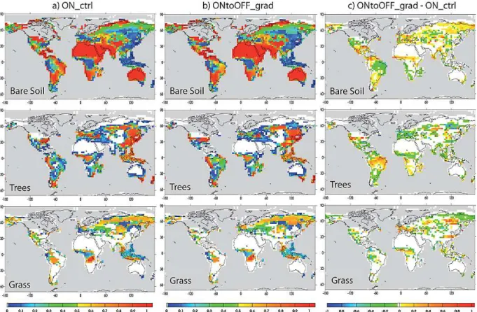
The performance of ORCHIDEE in simulating the glacial vegetation has been previously described by Woillez et al. (2011). Figure 3a presents the total forest, grass and bare soil fractions simulated in ON ctrl (corre-sponding to simulation LGMG in Woillez et al., 2011). ORCHIDEE correctly reproduces the main features of glacial vegetation, with high grass fractions over Siberia, in agreement with pollen data, indicating the dominance of steppic vegetation (Prentice et al., 2000), and the reduction of tropical forests compared to present-day, particularly over the Amazon Basin, where tree fractions are lower than 30 %. The main biases are an important overestimation of the bare soil fractions over India, southern Africa and South America, as well as an overestimation of the remaining tree fractions over Western Europe, eastern Eurasia and the Atlantic coast of North America.
The vegetation simulated at the end of ONtoOFF grad is presented in Fig. 3b (absolute vegetation fractions) and Fig. 3c (anomalies). The main differences between ON-toOFF grad and ON ctrl are an increase of forests over East Brazil, a decrease over central America and equatorial Africa, a reduction of forests over Western Europe, replaced by grasses, and a decrease of grasses over the Beringia re-gion. The increase of forest over South America at the ex-pense of the bare soil fraction is due to the strong increase of precipitation over this area in response to the displacement of the ITCZ (Fig. 2b). The opposite trend is simulated at the end of OFFtoON grad and OFFtoON fast compared to ON ctrl: the decrease in precipitation leads to a decrease in trees frac-tions (Fig. 4a, b). This result is in qualitative agreement with pollen data for South America (Hessler et al., 2010). The records with sufficiently high resolution to investigate the sponse of vegetation to millennial-scale variability in this re-gion are rather sparse, however a few sites from the northern and southern present-day limit of the ITCZ support the hy-pothesis of a southward migration of the ITCZ during HE events: in the Cariaco Basin, interstadials are characterized by an expansion of forests and stadials by the dominance of savannah, whereas records from northeastern Brazil show
the opposite trend, with increasing forest taxa during some HE events, indicating wetter conditions (Hessler et al., 2010). Both K¨ohler et al. (2005) and Menviel et al. (2008) simulate only small changes in the vegetation of South America in re-sponse to an AMOC collapse, due to limited changes in the position of the ITCZ. Our results are in qualitative agreement with the findings of Bozbiyik et al. (2011), showing a strong decrease in precipitation and consequently in terrestrial car-bon over the north of South America. However, they do not simulate a vegetation increase over Brazil. These differences in our results and previous studies highlights the interest of further investigation in the tropical response to AMOC changes, to assess quantitatively the contribution of tropical vegetation to changes in the carbon cycle during Heinrich events.
The vegetation response over Europe, with regression of forest and development of C3 grass when the AMOC col-lapse and opposite response when the AMOC recovers, is investigated in detail in the following sections.
4 Climatic response to changes of the AMOC over
Western Europe
Before investigating the European vegetation response to the climatic changes related to the AMOC collapse and re-sumption, we present this climatic response in more details in the following sections. We first compare the tempera-ture and precipitation simulated by IPSL CM4 in ON ctrl to the reconstructions from Wu et al. (2007) and then present the climatic changes in ONtoOFF grad, OFFtoON grad and OFFtoON inst.
4.1 Model-data comparison for the LGM control run
4.1.1 Temperature
Fig. 3.Fractions of bare soil, trees and grass (between 0 and 1) simulated by ORCHIDEE in(a)ON ctrl (average over 500 yr of run),(b) ONtoOFF grad (average over the last 200 yr of run) and(c)differences between ONtoOFF grad and ON ctrl.
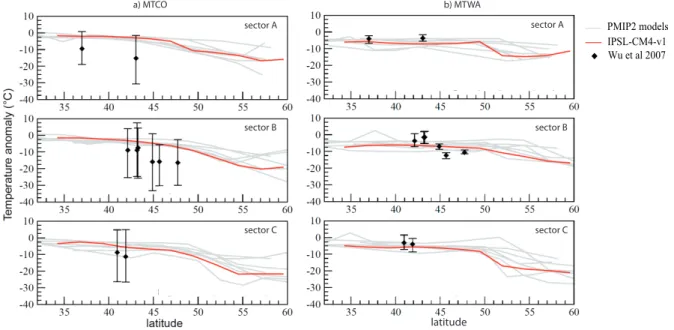
similar to those from the other models of the PMIP2 data base (in grey in Fig. 5).
4.1.2 Precipitation
Model-data comparison for anomalies in annual precip-itation in ON ctrl compared to the reconstructions of Wu et al. (2007) are presented in Fig. 6. The model sim-ulates annual precipitations similar or slightly above the present-day values for the three longitude bands considered. These values are within the uncertainty range of the recon-structions by Wu et al. (2007). However, precipitation over the Iberian peninsula are probably overestimated since the simulated values exceed the mean reconstruction by about 500 mm yr−1(Fig. 6, sector A, 43◦N). Temperatures simu-lated for this region are also overestimated by 10◦C (MTCO,
see Fig. 5a) compared to Wu et al. (2007) reconstructions, suggesting an overestimation of the advection of relatively warm and humid air from the ocean. This is consistent with a strong AMOC, which is more active than estimated from reconstructions (McManus et al., 2004; Piotrowski et al., 2005).
4.2 Response to the AMOC collapse and recovery
4.2.1 Temperature
The evolution of the mean annual temperature inland over Western Europe in ONtoOFF grad follows the gradual col-lapse of the AMOC, with a decrease from about 6◦C (in-terannual standard deviation: 0.75◦C) in ON ctrl to 4.3◦C (interannual standard deviation: 0.76◦C) over the last 400 yr of ONtoOFF grad (Fig. 1b). The comparison of Fig. 1a and Fig. 1b shows there is no lag between the temperature evolu-tion and the AMOC strength. For both variables, equilibrium is reached at the same time.
The anomaly of temperature observed in the North At-lantic (−4◦C in ON ctrl compared to ONtoOFF grad at
Fig. 4.Differences in the fractions of bare soil, trees and grass simulated by ORCHIDEE at the end of (a)OFFtoON grad and (b) OFFtoON fast compared to ON ctrl. OFFtoON grad: average over the last 30 yr of the run. OFFtoON fast: average over the last 20 yr of the run. ON ctrl: average over 500 yr of run.
Iberian Atlantic margin to only −1.5 to −1◦C in central France. MTCO anomalies in eastern France, Germany and Italy are not statistically significant. The decrease in MTWA is always smaller in amplitude than−1.5◦C, except for the
north and west of France, south-west Iberia and the North At-lantic coast of Iberia (−2 to−2.5◦C). The cooling associated to the AMOC collapse is stronger than the cooling simulated by Kageyama et al. (2005) with the same atmospheric model by prescribing SST anomalies of−4◦C in the North Atlantic to mimic the Heinrich event 1. In their study, MTCO was re-duced by less than 2◦C on the Atlantic side over Iberia, and less than 1◦C in central Iberia and the French Atlantic coast. However, the cooling in the MTCO simulated in this study at the end of ONtoOFF grad is still too small when compared to palynological reconstructions based on the modern analogue technique (Guiot, 1990). For H1 around the Alboran Sea for instance (ODP site 976), the reconstructed anomalies
com-pared to the LGM are between −5 to−15◦C (Kageyama et al., 2005; Combourieu-Nebout et al., 2009b). The simu-lated decrease in the MAT is closer to reconstructions of a decrease of about−2.6◦C (N. Combourieu-Nebout, personal
communication, 2012). However, it is known that the recon-structions based on the modern analogue technique have a tendency to underestimate the MTCO (Combourieu-Nebout et al., 2009b; Wu et al., 2007). Moreover, the lack of mod-ern analogue of the LGM vegetation adds uncertainties to the method, which in addition does not take the effect of low CO2on vegetation into account.
a) MTCO b) MTWA
IPSL-CM4-v1 Wu et al 2007 PMIP2 models
latitude
sector A sector A
sector B sector B
sector C sector C
Fig. 5.Difference in(a)the mean temperature of the coldest month (MTCO) and(b)mean temperature of the warmest month (MTWA) between the LGM and present-day simulated by IPSL CM4 (red) and other GCMs from the PMIP2 project (grey), for 3 longitude bands over Western Europe, between 32◦and 60◦N. The limits of the three sectors are plotted in Fig. 8. Sector A: lon =−15/-2◦, Sector B: lon =−2/10◦, Sector C: lon = 10/20◦. Black diamonds are MTWA and MTCO values reconstructed by Wu et al. (2007) with the associated uncertainty range.
35 40 45 50 55 60
-1000 -500 0 500 1000
35 40 45 50 55 60
-1000 -500 0 500 1000
IPSL-CM4-v1 Wu et al 2007
35 40 45 50 55 60
latitude -1000
-500 0 500 1000
Precipitation anomaly (mm/year)
PMIP2 models sector A
sector B
sector C
Fig. 6.Difference in annual precipitation (mm yr−1) between the LGM and present-day simulated by IPSL CM4 (red) and other GCM from the PMIP2 project (grey), for 3 longitude bands over Western Europe, between 32◦and 60◦N. The limits of the three sectors are plotted in Fig. 8. Sector A: lon =−15/−2◦, Sector B: lon =−2/10◦, Sector C: lon = 10/20◦. Black diamonds are precipi-tation values reconstructed by Wu et al. (2007) with the associated uncertainty range.
relatively warm air from the south-west to Western Europe, as mentioned in Sect. 3 (see also Kageyama et al., 2009).
When the AMOC gradually recovers in OFFtoON grad the mean annuel temperature rises again and stabilises
slightly above the value of ON ctrl. Similarly, in OFFtoON fast the mean annual temperature follows the AMOC evolution, the temperature abruptly rising by about 2.5◦C (Fig. 1b). Thus the impact of AMOC changes on European temperature is clearly unlinear since an AMOC collapse from 15 to 0 Sv leads to a temperature decrease of about 2◦C, whereas an increase from 15 to 30 Sv leads to a rise in temperature of about 1◦C.
4.2.2 Precipitation
When the AMOC collapses, we observe a gradual decrease in mean annual precipitation from 700±35 mm yr−1 in ON ctrl to 580±32 mm yr−1in ONtoOFF grad over the last 400 yr of simulation (see Fig. 1c). The decrease in precipita-tion follows the decrease in the AMOC strength.
At equilibrium, the precipitation decrease in ONtoOFF grad compared to ON ctrl is between −110 and −200 mm yr−1 over France, around
−200 mm yr−1 in northern Iberia and −100/−150 mm yr−1 in southern Iberia. The strongest decrease occurs in NW Iberia, with
−337 mm yr−1(Fig. 8).
55
50 45
40
35
55
50 45
40 35
55
50 45
40 35
a
b
c
ONtoOFF_grad - ON_ctrl
°C
MAT
MTCO
MTWA
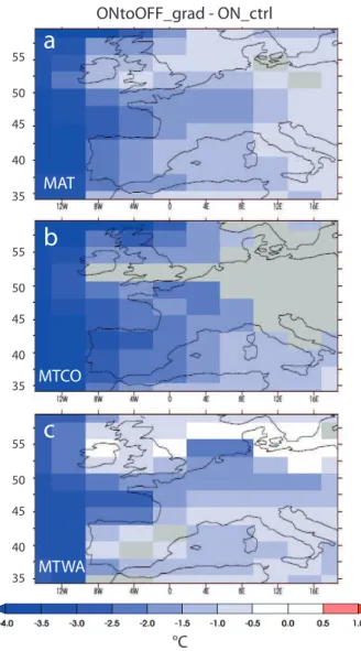
Fig. 7.Difference between ON ctrl and the end of ONtoOFF grad for(a)the mean annual temperature (MAT), (b) mean tempera-ture of the coldest month (MTCO) and (c)mean temperature of the warmest month (MTWA) (◦C). Grey areas are points where the difference is not significant at the 95 % level.
indicating a decrease of up to−214 mm yr−1 between H1 and the LGM in western Mediterranean for instance (Albo-ran ODP site 976, N. Combourieu Nebout and I. Dormoy, personal communication, 2012). Our results are closer to the amplitude of change reconstructed between a stadial with-out Heinrich event and an interstadial for the Alboran Sea by S´anchez-Go˜ni et al. (2002).
When the AMOC recovers, in OFFtoON grad and OFFtoON fast, the mean annual precipitation rises again and reaches about 730 mm yr−1at the end of OFFtoON grad and more than 750 mm yr−1at the end of OFFtoON fast, i.e. an increase of only 30 and 50 mm yr−1, respectively, compared to ON ctrl (Fig. 1c). The impact of the very high circulation rate of the AMOC at the end of OFFtoON fast compared
Fig. 8. Difference in annual precipitation (mm/year) between ON ctrl (average over 500 yr) and the end of ONtoOFF grad (av-erage over the last 200 yr of the run). Grey areas are points where the difference is not significant at the 95 % level.
to ON ctrl on European precipitation is thus much smaller than the impact when the AMOC collapses (ONtoON grad). Thus, similarly as for temperatures, the impact of AMOC on precipitation for changes around the value of ON ctrl is not linear.
5 Response of the European glacial vegetation to abrupt AMOC changes
5.1 Glacial vegetation in the control run
5.1.1 Model-data comparison for the LGM control run
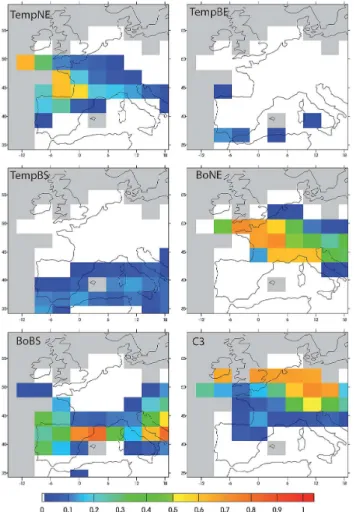
Fig. 9.Fractions of grid cells occupied by the different PFTs (annual maximum, between 0 and 1) simulated by ORCHIDEE in ON ctrl over Western Europe. The values are averages over the last 500 yr of the run. PFT acronyms: see Table 1. Grey areas are occupied by ocean or ice sheets.
When compared to pollen reconstructions, the vegeta-tion simulated by ORCHIDEE for the LGM appears to be closer to an interstadial than to a LGM vegetation. In-deed, pollen data for the LGM indicate the dominance of steppe-tundra vegetation over France (Fletcher et al., 2010), a herbaceous-dominant environment with Pinus and scattered pockets of deciduous trees in Iberia (Roucoux et al., 2005; Naughton et al., 2007), and shrubby vegetation with high values for semi-desert taxa in southern Iberia (Fletcher and S´anchez-Go˜ni, 2008), associated withCedar forest at high altitude (Combourieu-Nebout et al., 2009b). Thus our results for the Mediterranean, showing only small tree fractions, are in qualitative agreement with data, despite the lack of grasses, but further north forests are clearly overestimated. ORCHIDEE simulates a clear N / S gradient in vegetation, with semi-desertic vegetation in southern Iberia, BoBS forest in northern Iberia then gradually replaced by TempNE and BoNE over France and finally C3 grass. This gradient can be
compared to the gradient observed in pollen data by S´anchez-Go˜ni et al. (2008) for interstadials. They show a progres-sive transition from deciduous Mediterranean and temper-ate forests in Iberia to boreal forests with moreBetulaand
Pinusover France. Forest fractions in ON ctrl are overesti-mated even for an interstadial, but ORCHIDEE qualitatively reproduces the transition between broadleaf and needleleaf forests. The main discrepancy with pollen data for an inter-stadial is the high fractions of BoBS over Iberia, which can be at least partly attributed to the systematic overestimation of this PFT in ORCHIDEE (see Woillez et al., 2011). For the Adriatic region, LGM records indicate landscapes occu-pied by semi-desert taxa at low elevation and the presence of conifers at high altitudes, while deciduous forests were only poorly represented (Combourieu-Nebout et al., 1998). Our results are only in partial agreement with this reconstruction. ORCHIDEE reproduces correctly the absence of temperate PFTs and presence of BoNE (40 %), but grasses are clearly underestimated and BoBS overestimated (40 to 70 %), a gen-eral bias of the ORCHIDEE model (Woillez et al., 2011).
However, model-data comparison for vegetation can only remain qualitative, due to the coarse resolution of the vege-tation model, related to the coarse resolution of the climate model forcings. Particularly, the pollen record at one site can reflect the surrounding vegetation at different elevations, and the model does not allow us to consider vegetation changes with altitude within a grid box.
The overestimation of forest in Western Europe for the LGM is a common bias in vegetation simulations (see K¨ohler et al., 2005; Kageyama et al., 2005; Menviel et al., 2008). For the present study, this excess of forest can be partly attributed to the bias in the climatic forcings, too warm and wet com-pared to reconstructions (see Sect. 4.1).
5.1.2 Variability of glacial vegetation over Western Europe
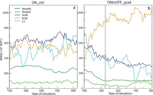
Fig. 10.Temporal evolution of the area occupied by each PFT over Western Europe (lat = 32/60◦, lon =−15/20◦) in(a)ON ctrl and(b) ONtoOFF grad (103km2, values are averages over 10 yr of run). The vertical grey bar indicates the full AMOC collapse. PFT acronyms: see Table 1. The area of TempBE remains below 20×103km2and this PFT has been omitted on both graphs.
given PFT, and leads to a decrease in productivity, but they did not investigate the response to climatic variability. The high vegetation variability observed in ON ctrl can be at-tributed to the increased sensitivity of vegetation to drought or cold temperatures under low CO2. Therefore, threshold conditions for survival are probably more often crossed than they are under modern CO2, when the tolerable climatic range is broader.
5.2 Vegetation response to AMOC changes
5.2.1 Collapse of the AMOC
Gradual collapse
Figure 10b gives the temporal evolution of the area occu-pied by each PFT in ONtoOFF grad. All PFTs react imme-diately to the change in climate due to the gradual collapse of the AMOC. However, equilibrium is not reached at the same time for each PFT. The evolution of TempNE and TempBS follows the decrease of the AMOC and the areas of these two PFTs reach their minimum in 250 yr. The slight increase of TempBS over the last 200 yr of the run corresponds to its development over only one grid cell in southwest Iberia and is therefore not really significant. BoNE reach equilib-rium after about 500 yr of simulation and their area stabi-lizes at 300×103km2(600×103km2in ON ctrl). The de-crease of BoBS starts immediately at the beginning of the
AMOC collapse, but given the high variability of this PFT in ON ctrl, the decrease only gets significant after about 500 yr of simulation, with values around 200×103km2(vs gener-ally more than 400×103km2in ON ctrl, cf. Fig. 10a). Bo-real forests thus continue to regress during about 200 yr after climatic equilibrium (see Fig. 1b, c for the temporal evolu-tion of the mean annual temperature and precipitaevolu-tion over Europe during ONtoOFF grad). C3 grasses essentially ex-pand over areas primarily occupied by forests, their temporal evolution is anti-correlated with the one of the tree PFTs. Equilibrium is reached after about 400–500 yr of simulation, around 1000×103km2(500–600×103km2in ON ctrl).
Fig. 11.Vegetation fractions (annual maximum) simulated by OR-CHIDEE at the end of ONtoOFF grad. The values are means over the last 200 yr of the run. PFT acronyms: see Table 1. Grey areas are occupied by ocean or ice sheets.
patches having fractions around 10 % only, but they subsist in the east, with fractions between 20 to 40 %. Correlatively to this general regression of tree PFTs, C3 grass expands in France, Italy and northern Iberia.
The regression of forests and the development of grasses is in qualitative agreement with pollen data (see Sect. 1). How-ever, ORCHIDEE still overestimates forests in south-west France and overestimates the effect of the aridity simulated by IPSL CM4 over Iberia since the west and south of the peninsula are dominated by bare soil, a bias already present in ON ctrl.
Our results are also in qualitative agreement with Kageyama et al. (2005). However, the vegetation simulated at initial state in their study is quite different from ours, with smaller tree fractions over France and almost no trees over Iberia, whereas grass fractions are much higher, with about
30 % in central France and 20 % in Iberia. As a result, in their study the “H1” climate leads to forest regression over France only, and also to a decrease in grass fractions both over France and Iberia.
Comparison to an instantaneous collapse
In order to assess the sensitivity of the vegetation to the rate of the AMOC collapse, we now compare the temporal evo-lution of the total area covered by forest (Fig. 12a) and the area covered by C3 grass (Fig. 12b) in response to a gradual (ONtoOFF grad) or instantaneous (ONtoOFF inst) AMOC collapse. How long is the lag between climate and vegetation when the change in climate corresponding to the “off” state of the AMOC is imposed instantaneously?
In ONtoOFF grad, the forested area gradually decreases from 1600×103km2 to 800×103km2 within 300 yr of simulation, remains stable during 300 yr, then briefly col-lapses to about 600×103km2 before increasing again at 800×103km2and finally decreases at 600×103km2at the end of the run. The high variability of forest cover, already described previously, is thus also present when the AMOC is collapsed and makes it difficult to precisely determine when the vegetation has reached its final state. We can consider that the equilibrium is reached after about 500–600 yr of simula-tion, i.e. about 200–300 yr after the AMOC full collapse.
When the climate for a collapsed AMOC is imposed in-stantaneously (ONtoOFF inst), as could be expected the de-crease in forested areas occurs more rapidly. It starts with an abrupt shift to 1250×103km2during the first 25 yr of simu-lation, followed by a more gradual decrease and equilibrium is reached after about 200 yr of simulation. Hence an instan-taneous climate change corresponding to an AMOC collapse does not immediately kill all the trees. Rather, the gradual re-gression of forest cover after the instantaneous change of cli-mate appears to be linked to the succession of unfavourable years over a long period.
Thus, in both simulations, a time lag of about 200 yr is observed between the equilibrium state of the AMOC and the equilibrium of forested areas. The evolution of the C3 grass area is different, since the rate of increase is approx-imately the same in ONtoOFF grad and ONtoOFF inst. In both simulations, the total area gradually increases from 350×103km2to 1000×103km2within 400 yr. This appar-ent similar evolution actually hides spatial differences, with a slower spatial expansion of C3 grasses in ONtoOFF grad, but with higher fractions than in ONtoOFF inst.
5.2.2 Relative impact of changes in temperature and precipitation during a gradual collapse of the AMOC on forest cover
Fig. 12. Area of Western Europe (lat = 32/60◦, lon =−15/20◦) occupied by (a) tree PFTs and (b) grass in ON ctrl (black), ONtoOFF grad (blue), ONtoOFF inst (orange), OFFtoON grad (green), OFFtoON fast (red), OFFtoON inst (turquoise). The ver-tical grey bars indicate when the AMOC is fully collapsed in ON-toOFF grad.
a first step towards understanding the reasons for these veg-etation changes, we investigate the relative impact of tem-perature and precipitation changes in ONtoOFF grad on Eu-ropean vegetation. We first compare the total area covered by TempNE, BoNE and BoBS in ON ctrl, ONtoOFF temp, ONtoOFF precip and ONtoOFF grad (Fig. 13).
For both TempNE and BoNE (Fig. 13a, b), changes in precipitation alone (ONtoOFF precip) are not sufficient to drive the decrease observed in ONtoOFF grad. For BoNE, the curves of ON ctrl and ONtoOFF precip are even almost exactly the same. On the contrary, when we consider ON-toOFF temp, TempNE and BoNE areas decrease more or less in the same way as in ONtoOFF grad. We can conclude that for needleleaf evergreen trees, for which the highest fractions are over France, the area changes when the AMOC collapse are caused by temperature changes and not by precipitation changes.
The area occupied by BoBS (Fig. 13c) in ONtoOFF precip and ONtoOFF temp does not really stand out of the
vari-ability observed in ON ctrl. Areas for the last 50 yr of ON-toOFF precip and ONON-toOFF temp are approximately the same (400–500×103km2), i.e. reduced compared to the area in ON ctrl (500–600×103km2) over the same period, though still within the variability of ON ctrl, whereas in ONtoOFF grad BoBS area is below 400×103km2. Thus, at European scale both temperature and precipitation play a role in the evolution of this PFT in ONtoOFF grad. This result can be refined when considering two smaller regions where BoBS are abundant in ON ctrl: Iberia and the Ital-ian and Adriatic regions. In Italy (Fig. 14b), changes in temperature alone lead to an increase of BoBS area, from 100×103km2 to 150–200×103km2, whereas changes in precipitation alone tend to make the BoBS area decrease. The respective impact of temperature and precipitation changes compensate and in ONtoOFF grad the area occupied by BoBS is not different from ON ctrl. The results are differ-ent for Iberia (Fig. 14a): the evolution of the BoBS area in ONtoOFF precip is similar to ON ctrl, and the evolution in ONtoOFF temp similar to ONtoOFF grad, which shows that temperature change is the main driver of BoBS decrease over the peninsula in ONtoOFF grad.
Thus, despite the relatively small decrease in tempera-tures in ONtoOFF grad compared to ON ctrl (see Fig. 7), the cooler temperatures are the main driver of the evolution of the area of the different tree PFTs (TempNE, BoNE, BoBS) in the west of Western Europe.
0 100 200 300 400 100
150 200 250 300
0 100 200 300 400 200
300 400 500 600 700
a) TempNE
b) BoNE
c) BoBS
A
rea (103
km
2)
A
rea (103
km
2)
150 250 350 450 550 150 250 350 450 550
0 100 200 300 400
0 100 200 300 400 0
200 400 600
ON_ctrl
ONtoOFF_grad ONtoOFF_temp ONtoOFF_precip
c) BoBS
Years of simulation
A
rea (103
km
2)
150 250 350 450 550
Years of simulation
Fig. 13.Area of Western Europe (lat = 32/60◦, lon =−15/20◦) occupied by(a)Temperate needleleaf evergreen;(b)Boreal needleleaf ev-ergreen;(c)Boreal broadleaf summergreen trees in ON ctrl (black), ONtoOFF grad (blue), ONtoOFF precip (red) and ONtoOFF temp (orange). The vertical grey bars indicate when the AMOC is fully collapsed in ONtoOFF grad.
5.2.3 Recovery of the AMOC
When the AMOC gradually recovers (OFFtoON grad), the forested area is back to the level of control values at the end of the run (Fig. 12a). However, contrary to the evolution of temperature and precipitation (Fig. 1b, c) no plateau is ob-served in the curve at the end of the run and the area covered by tree PFTs is probably not at equilibrium with the final cli-mate of OFFtoON grad, suggesting a lag of several decades between climate and vegetation. The area occupied by grass at the end of OFFtoON grad (Fig. 12b) remains higher by about 100×103km2than the mean level in ON ctrl, but this value is within the range of variability of the control run.
When the climate is set back to the control state instanta-neously (OFFtoON inst), both forest and C3 grass areas are back to the levels of ON ctrl within a century. This duration corresponds to the lag between climate and vegetation. We could have expected grass to respond faster than trees, but they actually reflect the evolution of forests and regress on areas where tree fractions increase.
The evolution of the areas covered by trees and grass in OFFtoON fast, for which the AMOC jumps from 0 to 30 Sv within 150 yr, is quite similar to the one simulated in OFFtoON inst. Final states are also similar, despite the very
different AMOC strength. This result is not very surprising, given the limited impact of this high AMOC level on the cli-mate of Western Europe compared to ON ctrl (Figs. 1 and 2). However, the global results presented in Fig. 12 hides spatial differences in the area covered by the different PFTs. At the end of OFFtoON fast compared to ON ctrl, BoNE fractions are smaller over France, Germany and the North of Italy, re-placed by BoBS and C3 grass. C3 grass extension decreases on the Atlantic French coast where BoBS and TempNE in-crease (results not shown). The change in climate at the end of OFFtoON fast compared to ON ctrl leads to a reorgani-sation of the distribution of the PFTs and modifications of the composition of forested areas, which are unseen in the evolution of the global forested area.
6 Discussion and conclusion
100 200 300 400 0
100 200 300
ON_ctrl ONtoOFF_grad ONtoOFF_temp ONtoOFF_precip
0 100 200 300 400
0 50 100 150 200
ON_ctrl ONtoOFF_grad ONtoOFF_temp ONtoOFF_precip
a) Spain
b) Italy & Adriatic
Years of simulation
A
rea (103
km
2)
A
rea (103
km
2)
150 250 350 450 550
150 250 350 450 550
Fig. 14.Surface occupied by boreal broadleaf summergreen trees over (a) Spain and (b) Italy + Adriatic in ON ctrl (black), ON-toOFF grad (blue), ONON-toOFF precip (red) and ONON-toOFF temp (or-ange). The vertical grey bars indicate when the AMOC is fully col-lapsed in ONtoOFF grad.
To investigate those questions, we have used the outputs of freshwater hosing experiments which have been performed under LGM conditions with the IPSL CM4 AOGCM, to sim-ulate a collapse and recovery of the AMOC at different rates. The different resulting climates have been used to drive the ORCHIDEE DGVM off-line and investigate the dynamical response of the glacial vegetation, with a special focus on the changes over Western Europe.
The glacial vegetation simulated by ORCHIDEE over Eu-rope for the LGM control simulation, in which the AMOC is active, is characterised by an overestimated forest cover, consistent with the overestimation of temperature and precip-itation over Western Europe in IPSL CM4. The high forest fractions and the transition from broadleaf PFT in the south to needleleaf and then to grasses with increasing latitudes is more in agreement with pollen data for an interstadial than for the LGM. Our 1000 yr of LGM control simulation also shows a high interannual variability of the areas occupied by the boreal needleleaf evergreen and the boreal broadleaf summergreen trees. The glacial vegetation seems to be close
to climatic thresholds and therefore very sensitive to climatic variability. Temperature seems to be the main driver of this variability, however further investigation is required to better understand the mechanism at play since no obvious correla-tion between annual or monthly temperature and the evolu-tion of these two PFTs could be found.
When the AMOC collapses, IPSL CM4 simulates the expected thermal bipolar see-saw between the two hemi-spheres, with cooling in the North Atlantic and warming in the Southern Ocean and a southward migration of the ITCZ. The opposite climatic response is simulated for the AMOC resumption. Temperature anomalies simulated over the North Atlantic do not propagate far inland over Western Europe be-cause of the development of a cyclonic (resp. anticyclonic) anomaly which brings warm (resp. cool) air over the conti-nent when the AMOC collapses (resp. recovers).
The climatic changes associated to an AMOC collapse lead to forests regression over Western Europe, replaced by grasses in qualitative agreement with pollen data for HE events. Sensitivity tests show that this European forest re-gression is mainly driven by the cooling in temperatures, al-though this cooling is limited to a few ◦C on average. For most parts of Western Europe, precipitation decrease appears to have only a small impact. Thus, our model vegetation is highly sensitive to temperature changes and a tempera-ture decrease as strong as reconstructed from pollen data (e.g. Combourieu-Nebout et al., 2009b) is not required to drive important vegetation changes. This result suggests that the amplitude of climatic changes reconstructed from pollen data for HE events may be overestimated. However, the re-maining simulated forest fractions simulated by ORCHIDEE at the end of the AMOC collapse are still overestimated over France compared to pollen data. Thus, even if climatic re-constructions may be biased, temperature and/or precipita-tion changes are probably nevertheless still underestimated by the AOGCM.
A more detailed statistical analysis of our results is re-quired to better understand which temperature parameters drive the European vegetation changes. Is it an increase in the frequency of very cold temperatures at the daily scale? Or the long-term impact of temperature conditions less favourable, but not extreme? Another interesting point would be to inves-tigate changes in the amplitude of the seasonal cycle, an im-portant parameter for various Mediterranean and temperate species which is known to have changed during HE events in the western Mediterranean region (Combourieu-Nebout et al., 2009a).
The forest regression recorded in pollen data could indeed be driven by the temperature decrease and the development of xeric plants, among other types of grasses, favoured by the decrease in precipitation. A more complete description of the vegetation in ORCHIDEE would be needed to examine these hypotheses.
Our results on the timing of the vegetation response to AMOC changes are summarized in Fig. 15. The mean annual temperature (Fig. 15a) and the mean annual precipitation (Fig. 15b) both respond synchronously to AMOC changes. Both graphs show a large interannual variability of temper-ature and precipitation values for a given AMOC strength, but the relationship appears to be linear for AMOC values between 0 and 20 Sv. Temperature and precipitation values for AMOC strengths above 20 Sv are close to control values, showing the limited impact of a transient hyperactive AMOC on the European climate. The different values of forested areas in ONtoOFF grad, OFFtoON grad and OFFtoON fast for AMOC strength between 7 and 12 Sv (Fig. 15c) clearly show a time lag between vegetation and AMOC changes. The total forested area being less variable than temperature and precipitation for a given AMOC strength, vegetation sen-sitivity to AMOC changes is also more visible. Given the synchronicity between the evolution of the AMOC and of the European climate, the time lag between the AMOC and vegetation is related to vegetation dynamics. We have shown that at the European scale this time lag is about 200 yr for an AMOC collapse and 100–200 yr for the AMOC recov-ery. The vegetation obtained for a very fast increase of the AMOC from 0 to 30 Sv is close to control state, partly be-cause the simulation is not at equilibrium and partly bebe-cause of the limited continental impact of this hyperactive AMOC. The study of abrupt climatic events in marine cores from the Alboran Sea shows that the different DO and Heinrich events have very different signatures, both in the SST and in the pollen records (e.g. Fletcher and S´anchez-Go˜ni, 2008). The temporal resolution of the analyses carried out on the cores does not always allow a precise comparison of the tim-ing of the ocean and vegetation response to abrupt events, and only few marine cores have a resolution good enough for such a comparison. The study of S´anchez-Go˜ni et al. (2002) shows a perfect coupling between terrestrial and marine changes for the Heinrich event 4 (H4) in the Alboran Sea, with a temporal resolution of 200 yr. The same study also shows that the timing of changes for two regions not so far from one another can be quite different: for H4, the maxi-mum of steppic plants is reached at the onset of the event in the Alboran Sea, but only in the second part of the event on the Atlantic side of SW Iberia. Data from Combourieu-Nebout et al. (2009b), with a time resolution refined to 20– 40 yr during abrupt events confirm the synchronicity be-tween marine and terrestrial changes for HE events in the Alboran Sea. Other Atlantic and Mediterranean cores also record synchronous marine and continental changes for H2
(Combourieu-Nebout et al., 1998, 2002; Turon et al., 2003; Naughton et al., 2007).
The comparison of our results to pollen data can only be qualitative given the relatively coarse resolution of our model. Given the duration of our experiment, which is short compared to the time resolution of most of the available pollen records, our results for a collapse of the AMOC are in qualitative agreement with data for a Heinrich event. The rapidity of the vegetation response is also in agreement with the pollen record of Allen et al. (1999), showing vegetation changes occurring in less than 200 yr in the South of Italy. The lag of more than a century simulated when climatic con-ditions for an inactive AMOC are imposed instantaneously was somehow unexpected since trees can be killed within only a few years. This result suggests that the decrease of forest is driven by the succession of unfavourable years over a long period rather than by the abrupt crossing of a bio-climatic threshold. Besides, the amplitude of climate change reconstructed from pollen data for a Heinrich event is larger than the changes simulated by IPSL CM4. A more drastic climate change would probably reduce the lag of simulated vegetation changes with respect to climate changes, which could be tested by adding systematic temperature and/or pre-cipitation anomalies of different amplitudes to the forcing. Such an approach could allow for the establishment of a re-lationship between the amplitude of the climate change and the duration of the lag between climate and vegetation.
The time lag when the AMOC recovers could be expected since a forest obviously needs time to grow again, but this lag is much smaller than the several centuries needed for the regrowth of forests according to pollen data. In the south of Iberia (Alboran Sea site ODP 976) the forest maximum is reached 600 yr after the onset of DO 12 and 800 yr after the onset of DO 8. Vegetation changes in the Adriatic also occur over centuries, with about 400 to 1000 yr for the complete re-growth of forests after a minimum (N. Combourieu-Nebout, personal communication, 2012). This discrepancy might be related to the absence of simulation of pollen dispersal in the model. The regrowth of forests after a phase of severe regres-sion first requires the transport of seeds at places where trees have disappeared. The dispersal of seeds from small remain-ing trees refugia might takes decades or century, dependremain-ing on the distance between the refugia and the location consid-ered (e.g. Brewer et al., 2002).
Fig. 15. (a)Mean annual temperature (◦C),(b)mean annual precipitation (mm yr−1) and(c)area covered by trees (103km2) over Western Europe (lat = 32/60◦, lon =−15/20◦) vs NADW strength at 30◦S (Sv) for simulations ON ctrl (black), ONtoOFF grad (blue), OFFtoON grad (green) and OFFtoON fast (red). Each cross corresponds to the result for one year.
effect on regions where forests have disappeared. This hy-pothesis could be tested by comparing our present results to simulations with full coupling between climate and vegeta-tion.
The response of European vegetation to a very fast shift in the AMOC strength from 0 to 30 Sv, designed to mimic a DO event, is very close to the response to an instantaneous return to the climatic conditions of the control run. Simulat-ing an abrupt shift from a collapsed to a hyperactive AMOC is not necessary to qualitatively simulate the vegetation re-sponse to a DO, an abrupt return to initial conditions give the same results, which suggests that the equilibrium state of the glacial climate may correspond rather to interstadials than to stadials.
In any case, the disequilibrium between vegetation and cli-mate during our transient simulations suggests that the as-sumption of vegetation-climate equilibrium used in palyno-logical climate reconstructions may not be valid for time res-olution higher than a century. To simulate vegetation changes in agreement with pollen data, different climatic scenarios are possible, depending on the existence and duration of a lag between climate and vegetation changes. Thus, the use of dynamic vegetation models can provide some constraints
on abrupt changes on the continent, especially where pollen records are the only data available. Different rates and am-plitudes of changes in temperature and precipitation can be tested to establish which scenarios can lead to vegetation changes in agreement with pollen data, for both the change in composition and the speed of change.
Acknowledgements. The simulations have been run on the com-puter of the Centre de Calcul Recherche et Technologie (CCRT, France). We thank two anonymous reviewers for their comments to improve this manuscript.
Edited by: F. Joos
References
Allen, J., Brandt, U., Brauer, A., Hubbertens, H.-W., Huntley, B., Keller, J., Kraml, M., Mackensen, A., Mingram, J., Negendank, J., Nowaczyk, N., Oberh¨ansli, H., Watts, W., Wulf, S., and Zolitschka, B.: Rapid environmental changes in southern europe during the last glacial period, Nature, 400, 740–743, 1999. Alley, R. B., Anandakrishnan, S., and Jung, P.: Stochastic resonance
in the North Atlantic, Paleoceanography, 16(2), 190–198, 2001. Barker, S., Diz, P., Vautravers, M. J., Pike, J., Knorr, G., and
Hall, I.: Interhemispheric atlantic seesaw response during the last deglaciation, Nature, 457, 1097–1103, 2009.
Berger, A.: Long-term variations of daily insolation and Quaternary climatic changes, J. Atmos. Sci., 35, 2362–2367, 1978. Blunier, T., Chappellaz, J., Schwander, J., D¨allenbach, A., Stauffer,
B., Stocker, T., Raynaud, D., Jouzel, J., Clausen, H., Hammer, C., and Johnsen, S.: Asynchrony of Antarctic and Greenland cli-mate change during the last glacial period, Nature, 394, 739–743, 1998.
Bond, G. and Lotti, R.: Iceberg Discharges into the North Atlantic on Millennial Time Scales During the Last Glaciation, Science, 267, 1005–1010, 1995.
Bozbiyik, A., Steinacher, M., Joos, F., Stocker, T. F., and Menviel, L.: Fingerprints of changes in the terrestrial carbon cycle in re-sponse to large reorganizations in ocean circulation, Clim. Past, 7, 319–338, doi:10.5194/cp-7-319-2011, 2011.
Braconnot, P., Otto-Bliesner, B., Harrison, S., Joussaume, S., Pe-terchmitt, J.-Y., Abe-Ouchi, A., Crucifix, M., Driesschaert, E., Fichefet, Th., Hewitt, C. D., Kageyama, M., Kitoh, A., Laˆın´e, A., Loutre, M.-F., Marti, O., Merkel, U., Ramstein, G., Valdes, P., Weber, S. L., Yu, Y., and Zhao, Y.: Results of PMIP2 coupled simulations of the Mid-Holocene and Last Glacial Maximum – Part 1: experiments and large-scale features, Clim. Past, 3, 261– 277, doi:10.5194/cp-3-261-2007, 2007.
Braun, H., Christl, M., Rahmstorf, S., Ganopolski, A., Mangini, A., Kubatzki, C., Roth, K., and Kromer, B.:Possible solar origin of the 1,470-year glacial climate cycle demonstrated in a coupled model, Nature, 438, 208–211, 2005.
Brewer, S., Cheddadi, R., de Beaulieu, J., Reille, M., and contrib-utors, D.: The spread of deciduousQuercusthroughout Europe since the last glacial period, Forest Ecol. Manage., 156, 27–48, 2002.
Claussen, M., Ganopolski, A., Brovkin, V., Gerstengarbe, F.-W., and Werner, P.: Simulated global-scale response of the climate system to Dansgaard/Oeschger and Heinrich events, Clim. Dy-nam., 21, 361–370, 2003.
Clement, A. and Peterson, L.: Mechanisms of abrupt climate change of the last glacial period, Rev. Geophys., 46, RG4002, doi:10.1029/2006RG000204, 2008.
Combourieu-Nebout, N., Paterne, M., Turon, J.-L., and Siani, G.: A high-resolution record of the last deglaciation in the cen-tral Mediterranean Sea: palaeovegetation and palaeohydrological evolution, Quaternary Sci. Res., 17, 303–317, 1998.
Combourieu-Nebout, N., Turon, J.-L., Zahn, R., Capotondi, L., Londeix, L., and Pahnke, K.: Enhanced aridity and atmospheric high-pressure stability over the western Mediterranean during the North Atlantic cold events of the past 50 k.y., Geology, 30, 863– 866, 2002.
Combourieu-Nebout, N., Bout-Roumazeilles, V., Dormoy, I., and Peyron, O.: Persistent dryness events in the mediterranean along
the last 50 000 years, S´echeresse, 20, 210–216, 2009a.
Combourieu-Nebout, N., Peyron, O., Dormoy, I., Desprat, S., Beau-douin, C., Kotthoff, U., and Marret, F.: Rapid climatic variability in the west Mediterranean during the last 25 000 years from high resolution pollen data, Clim. Past, 5, 503–521, doi:10.5194/cp-5-503-2009, 2009b.
Crowley, T.: North Atlantic deep waters cools the southern hemi-sphere, Paleoceanography, 7, 489–497, 1992.
D¨allenbach, A., Blunier, T., Fl¨uckiger, J., Stauffer, B., Chappellaz, J., and Raynaud, D.: Changes in the atmospheric CH4 gradient between Grennland and Antartica during the Last Glacial and the transition to the Holocene, Geophys. Res. Lett., 27, 1005–1008, 2000.
Dansgaard, W., Johnson, S., Clausen, H., Dahl-Jensen, D., Gunde-strup, N., Hammer, C., Hvidberg, C., Steffensen, J., Sveinbjorns-dottir, A., and Jouzel, J.: Evidence for general instabilities of past climate from a 250-kyr ice-core record, Nature, 364, 218–220, 1993.
de Beaulieu, J. and Reille, M.: A long Upper Pleistocene pollen record from Les Echets, near Lyon, France, Boreas, 13, 111–132, 1984.
de Beaulieu, J. and Reille, M.: Long Pleistocene pollen sequences from the Velay Plateau (Massif Central, France), Veg. Hist. Ar-chaeobot., 1, 233–242, 1992a.
de Beaulieu, J. and Reille, M.: The last climatic cycle at La Grande Pile (Vosges, France) a new pollen profile, Quaternary Sci. Res., 11, 431–438, 1992b.
Ditlevsen, P. D., Andersen, K. K., and Svensson, A.: The DO-climate events are probably noise induced: statistical investiga-tion of the claimed 1470 years cycle, Clim. Past, 3, 129–134, doi:10.5194/cp-3-129-2007, 2007.
Elliot, M., Labeyrie, L., and Duplessy, J.-C.: Changes in North Atlantic deep-water formation associated with the Dansgaard-Oeschger temperature oscillations (60–10 ka), Quaternary Sci. Res., 21, 1153–1165, 2002.
EPICA Community Members: One-to-one coupling of glacial cli-mate variability in Greenland and Antarctica,Nature, 444, 195– 198, 2006.
Fletcher, W. and S´anchez-Go˜ni, M.-F.: Orbital- and sub-orbital-scale climate impacts on vegetation of the western Mediterranean basin over the last 48,000 years, Quaternary Res., 70, 451–464, 2008.
Fletcher, W., S´anchez-Go˜ni, M. F., Allen, J., Cheddadi, R., Combourieu-Nebout, N., Huntley, B., Lawson, I., Londeix, L., Magri, D., Margari, V., M¨uller, U., Naughton, F., Novenko, E., Roucoux, K., and Tzedakis, P.: Millennial-scale variability dur-ing the last glacial in vegetation records from Europe, Quat. Scie. Rev., 29, 2839–2864, 2010.
Fl¨uckiger, J., D¨allenbach, A., Blunier, T., Stauffer, B., Stocker, T., Raynaud, D., and Barnola, J.: Variations in atmospheric N2O
concentration during abrupt climatic changes, Science, 285, 227– 230, 1999.
Ganopolski, A. and Rahmstorf, S.: Rapid changes of glacial cli-mate simulated in a coupled clicli-mate model, Nature, 409, 153– 158, 2001.