www.atmos-chem-phys.net/11/4633/2011/ doi:10.5194/acp-11-4633-2011
© Author(s) 2011. CC Attribution 3.0 License.
Chemistry
and Physics
Vertical profiles of droplet effective radius in shallow
convective clouds
S. Zhang1, H. Xue1, and G. Feingold2
1Department of Atmospheric and Oceanic Sciences, School of Physics, Peking University, Beijing, China 2NOAA Earth System Research Laboratory, Boulder, Colorado, USA
Received: 8 December 2010 – Published in Atmos. Chem. Phys. Discuss.: 21 December 2010 Revised: 23 April 2011 – Accepted: 6 May 2011 – Published: 17 May 2011
Abstract. Conventional satellite retrievals can only provide information on cloud-top droplet effective radius (re). Given the fact that cloud ensembles in a satellite snapshot have dif-ferent cloud-top heights, Rosenfeld and Lensky (1998) used the cloud-top height and the corresponding cloud-toprefrom the cloud ensembles in the snapshot to construct a profile of rerepresentative of that in the individual clouds. This study investigates the robustness of this approach in shallow con-vective clouds based on results from large-eddy simulations (LES) for clean (aerosol mixing ratioNa= 25 mg−1), inter-mediate (Na = 100 mg−1), and polluted (Na = 2000 mg−1) conditions. The cloud-top height and the cloud-toprefrom the modeled cloud ensembles are used to form a constructed reprofile, which is then compared to the in-cloudreprofiles. For the polluted and intermediate cases where precipitation is negligible, the constructedreprofiles represent the in-cloud re profiles fairly well with a low bias (about 10 %). The method used in Rosenfeld and Lensky (1998) is therefore validated for nonprecipitating shallow cumulus clouds. For the clean, drizzling case, the in-cloudrecan be very large and highly variable, and quantitative profiling based on cloud-topre is less useful. The differences inre profiles between clean and polluted conditions derived in this manner are how-ever, distinct. This study also investigates the subadiabatic characteristics of the simulated cumulus clouds to reveal the effect of mixing onre and its evolution. Results indicate that as polluted and moderately polluted clouds develop into their decaying stage, the subadiabatic fractionfadbecomes smaller, representing a higher degree of mixing, andre be-comes smaller (∼10 %) and more variable. However, for the
clean case, smallerfad corresponds to largerre (and larger
Correspondence to:H. Xue ([email protected])
re variability), reflecting the additional influence of droplet collision-coalescence and sedimentation onre. Finally, pro-files of the vertically inhomogeneous clouds as simulated by the LES and those of the vertically homogeneous clouds are used as input to a radiative transfer model to study the effect of cloud vertical inhomogeneity on shortwave radiative forc-ing. For clouds that have the same liquid water path,reof a vertically homogeneous cloud must be about 76–90 % of the cloud-topreof the vertically inhomogeneous cloud in order for the two clouds to have the same shortwave radiative forc-ing.
1 Introduction
Aerosol-cloud interactions are recognized as one of the largest uncertainties in the prediction of climate change. Representation of shallow convection in climate models is a major challenge because the relevant spatiotemporal scales are on the order of tens to hundreds of meters and seconds, i.e., scales much smaller than those that can be resolved by climate models, both now and in the foreseeable future (e.g., Lohmann and Feichter, 2005; Wang and Penner, 2009). Recent studies have shown that the manner in which warm clouds and their interaction with aerosol particles are repre-sented by climate models has a marked effect on climate sen-sitivity – i.e., the Earth’s temperature response to a doubling of CO2.
lifetime through a reduction of drizzle, imposing an addi-tional cooling effect on the global climate system (Albrecht, 1989). However, the cloud lifetime effect and other processes such as the influence of aerosol on entrainment mixing are not well-understood (e.g., Jeffery and Reisner, 2006).
Quantification of aerosol-cloud interaction (ACI) is some-times expressed as ACI =−d ln re/d ln τ at fixed LWP, wherere is the cloud droplet effective radius, andτ is the aerosol optical depth (Feingold et al., 2001; Feingold, 2003). McComiskey and Feingold (2008) found that an error of 0.05 in ACI can lead to large changes in the estimation of the ra-diative forcing. The fact that many field observations and satellite measurements to date have shown that ACI is highly variable (e.g., Feingold et al., 2003; Breon et al., 2002) sug-gests that there is large uncertainty in cloud albedo forcing. This is partly because physical mechanisms may vary under different conditions and locations, but ACI is also quite sen-sitive to the method of remote re retrieval (Rosenfeld and Feingold, 2003) and to the aerosol proxy for cloud conden-sation nuclei (McComiskey et al., 2009). In general, in-situ and ground-based observations of ACI tend to be higher and closer to the theory of droplet activation than those from satellites.
The horizontal and vertical variability ofreimposes diffi-culty onreretrievals and hence uncertainty in ACI estima-tion. As shown in many field observations, droplet size not only exhibits horizontal heterogeneity, but also vertical strat-ification (e.g., Warner, 1955; Brenguier et al., 2000; Miles et al., 2000; Hudson and Yum, 2001; Twohy et al., 2005; Jiang et al., 2008; Lu et al., 2008; Arabas et al., 2009). The verti-cal stratification of droplet size must be resolved because it is central to both the cloud albedo and the precipitation pro-cess (Brenguier et al., 2003; Rosenfeld and Lensky, 1998). Although in situ measurements can resolve vertical profiles of droplet size, they cannot provide regional or global scale data sets for understanding and parameterization of aerosol effects on climate. Robust and widely applicable methods are needed for retrieving profiles of cloud dropletre. Ground-based remote sensing can retrieve droplet size profiles us-ing millimeter cloud radar, with a constraint of microwave-derived LWP and assuming a droplet size distribution model, a fixed spectral breadth, and a constant droplet number con-centration (Frisch et al., 1995). Measurements of re from satellite radiometers such as the Advanced Very High Reso-lution Radiometer (AVHRR) and Moderate ResoReso-lution Imag-ing Spectroradiometer (MODIS) tend to be confined to cloud top because a single near infrared (NIR) channel is more sen-sitive to the layer near cloud top rather than the lower layers (e.g., Nakajima and King, 1990). A recent study has revealed that the retrieval of droplet size can be strongly influenced by the vertical inhomogeneity of droplet size (Nakajima et al., 2010). Retrieving vertical profiles ofrefrom satellite ra-diometers has only become feasible in recent years for low-level, nonprecipitating stratiform clouds by assuming linear re profiles and with the use of MODIS shorter wavelength
measurements that penetrate deeper into the clouds (Chang and Li, 2002; Chen et al., 2008).
Because of the difficulty of deriving re profiles from conventional satellite measurements, Rosenfeld and Lensky (1998) and Lensky and Rosenfeld (2003) used the cloud-top height and the corresponding cloud-top re from the cloud ensembles in the satellite snapshot to construct a profile of re that can be used to represent the re profile in the absence of precipitation. In so doing, they assumed that cloud-top properties observed for cloud ensembles in the snapshot (each cloud having different cloud-top height and sampled at a different stage of the vertical growth) are similar to the properties of a single cloud as it grows through vari-ous heights (Arakawa and Schubert, 1974). This assumption of time-space exchangeability has been validated by Lensky and Rosenfeld (2006). The cloud-top height vs. cloud-top rerelationship for the snapshot was compared with the com-positereprofile for individual clouds tracked along their life-cycle, using 3-min satellite images. They confirmed that the composite properties from tracking the cells reproduce the properties in the snapshot. Because entrainment-mixing is significant for convective clouds, and because the top and the sides of convective clouds may experience different de-grees of mixing (e.g., Warner, 1955; Blyth et al., 1988; Blyth, 1993; Burnet and Brenguier, 2007; Small and Chuang, 2008; Jiang et al., 2008; Lu et al., 2008), cloud droplet size at cloud top and inside of clouds and clouds at different stages of the lifecycle may deviate from the adiabatic value to different degrees. However, if entrainment mixing is inhomogeneous, then cloud droplet size is likely independent on the degree of mixing (Freud et al., 2008). The assumption that cloud-topre acquired by satellites is representative of in-cloudre at the same height for shallow convective clouds, as used in Rosenfeld and Lensky (1998), will be tested here.
In global climate model parameterizations,reis usually as-sumed to be vertically fixed or dependent on cloud thickness. Brenguier et al. (2003) pointed out that cloud vertical strati-fication must be taken into account in climate model param-eterizations of cloud radiative properties and can be approx-imated with an adiabatic model for stratus clouds. It should also be noted that the stratified cloud model has been used to develop procedures for the retrieval of cloud geometrical thickness, liquid water content, and drop number concentra-tion from the measurement of cloud radiances for stratiform clouds (Sch¨uller et al., 2005). How to use this kind of cloud model for parameterization and retrieval in shallow convec-tive clouds remains uncertain because the mixing process can lead to significant changes in cloud microphysical properties (Warner, 1955).
simulations in this study are based on the Barbados Oceano-graphic and Meteorology Experiment (BOMEX), during which steady-state cumulus convection was observed for a period of several days. More details of the simulations can be found in Xue and Feingold (2006). The spatial variabil-ity ofreis investigated to shed light on implications for both satellite retrieval and model parameterization of the aerosol effects (Brenguier et al., 2003). We investigate whether the in-cloudreprofiles can be constructed using cloud-topreand the corresponding cloud-top height from satellite measure-ments for convective clouds. The in-cloud variability ofre is compared in each case to the variability due to aerosol ef-fects. The evolution ofre profiles and the degree to which reprofiles are affected by mixing are also studied. A plane-parallel radiative transfer model is then used to investigate the effect of cloud vertical inhomogeneity on shortwave ra-diative forcing. The model data and methods are described in Sect. 2. Results and discussions are presented in Sect. 3, and conclusions are summarized in Sect. 4.
2 Data and method
Data used in this study are model output from a set of large-eddy simulations of trade cumuli with aerosol mixing ratios ofNa= 25, 100 and 2000 mg−1(mixing ratio units of mg−1 are approximately equal to cm−3)that represent clean, in-termediate, and polluted conditions, respectively. Details of the LES model and the case are given in Xue and Fein-gold (2006). Precipitation is light in the clean case and negli-gible in the intermediate and polluted cases. We choose dif-ferent aerosol concentrations to see if thereprofiles have dif-ferent characteristics under non-precipitating and drizzling conditions. re is calculated based on the droplet size dis-tribution that is represented by 33 bins from 1–2500 µm ra-dius. The large-eddy simulations were performed in a doubly periodic, 6.4 km×6.4 km×3 km domain. The model
grid-spacing is1x=1y= 100 m, and1z= 40 m. All the simula-tions were run for six hours, but analysis was only performed over the last four hours. Model output was sampled every 5 min, thus 48 snapshots in the last four hours of simulation in each case were analyzed.
The areas where LWP exceeds 10 g m−2are considered as cloudy areas. We define cloud-toprein each cloudy column as thereat the highest grid point that has liquid water mix-ing ratioql>0.01 g kg−1. We use the cloud-topreand the corresponding cloud-top height from the modeled cloud en-sembles in 48 snapshots to construct anreprofile. This con-structedreprofile is then compared to thereprofile from all cloud samples in the 48 snapshots. The purpose is to test if the cloud-topre, measured from satellites, can represent the re well in clouds at the same height for convective clouds. Because cloud-top droplet size is usually affected by entrain-ment mixing, we also add two additional measures of cloud-top re to the analyses: one is there at one grid below the
highest grid point that hasql>0.01 g kg−1; the other is the maximumrein the column (usually several grid points below the highest grid point that hasql>0.01 g kg−1). Results us-ing different definitions of cloud-topre will be discussed in Sect. 3. The plane-parallel radiative transfer model SBDART (Santa Barbara DISTORT Atmospheric Radiative Transfer; Ricchiazzi et al., 1998) is used to investigate the shortwave radiative forcing of shallow cumulus clouds. The focus is on the effect of cloud vertical inhomogeneity, and so we ignore three-dimensional radiative effects, which were addressed by Zuidema et al. (2008). Because the simulated cumulus clouds cover heights betweenz= 600 m andz= 2200 m, but most clouds have cloud tops lower thanz= 1600 m, we use a solid cloud layer covering the height ofz= 600–1600 m in the SBDART model. The vertical inhomogeneity of the solid cloud layer is represented by 5 sublayers, each of which has a depth of 200 m. The liquid water content (LWC) andreof each sublayer is an average of the LES results in that layer for each of the simulated cases. We compare the shortwave ra-diative forcing of the vertically inhomogeneous clouds with that of the vertically homogeneous clouds that have the same LWP. The SBDART model also requires setup of the atmo-spheric profile, aerosols, surface model, etc. We select the tropical atmospheric profile, which is one of the six standard atmospheric profiles in the model. The aerosol optical depth in the cloud-free atmosphere is simply set to zero because we only investigate the difference of radiative forcings from a vertically homogeneous cloud and a vertically inhomoge-neous cloud. The surface model in SBDART is selected as ocean water. Solar zenith angle is varied from 0–90 degrees but only results for the 60 degree are shown here. We in-vestigate the effect of cloud vertical inhomogeneity on the radiative forcing over the wavelength range of 0.25–4.0 µm.
3 Results
3.1 reprofiles of cloud population
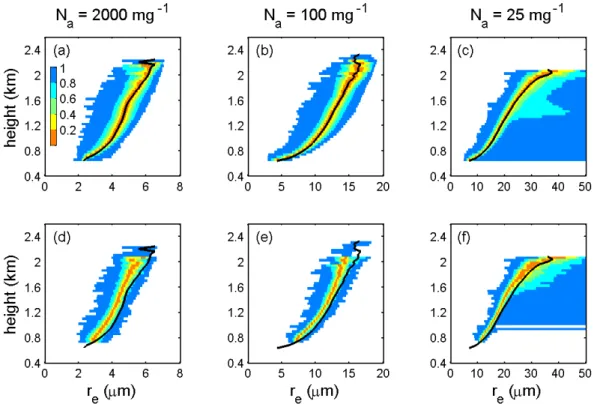
Figure 1 showsre profiles of the cloud population over the last 4 h of simulation. Thereprofiles from all cloud samples in each case are shown in Fig. 1a–c, and the 50th percentile of thereis shown as a reference (black lines). In the polluted and intermediate cases where precipitation is suppressed,re increases with height and also exhibits variability at each level (Fig. 1a, b). In the clean case where precipitation devel-ops,regenerally increases with height but with significantly higher variability at all levels (Fig. 1c). Thereprofile is com-plicated in the clean case due to droplet collision-coalescence and sedimentation. Note that for clarity the drizzle-mode drops larger than 50 µm radius (both inside of the clouds and below the cloud base) in the clean case are not shown (the scale of the x-axis is set to 50 µm).
Fig. 1. reprofiles of cloud population in the last 4 h of simulation in the polluted (Na= 2000 mg−1), intermediate (Na= 100 mg−1), and
clean (Na= 25 mg−1)cases.(a, b, c)reprofiles from all cloud samples.(d, e, f)Constructedreprofiles using cloud-topre. Different colors
represent different percentiles. (Orange: 40–60 percentiles; yellow: 30–40, 60–70 percentiles; green: 20–30, 70–80 percentiles; cyan: 10–20, 80–90 percentiles; blue: 0–10, 90–100 percentiles.) Notice that data points are few near cloud top so that only blue is used to represent 0-100 percentiles. The drizzle mode drops (larger than 50 microns) in clouds and below cloud base are not shown in the clean case for clarity. The 50th percentile of therefrom all cloud samples in each case are shown for reference (black lines).
samples is also shown as a reference (black lines). The con-structedreprofiles have similar properties to thereprofiles from all cloud samples, although with a low bias (as can be seen from the medianre in the constructedre profile com-pared to the 50th percentile ofrefrom all cloud samples in each case). This bias is about 0.5 µm (∼10 %) in the
pol-luted case, 1 µm (∼10 %) in the intermediate case, and 2 µm
(∼10 %) in the clean case. The constructedredoes represent the in-cloudre in the polluted and intermediate cases fairly well, with a low bias (∼10 %), providing evidence that the
cloud-top re from satellite measurements can generally be used for profilingre. Therefore the method used in Rosen-feld and Lensky (1998) is validated in this study for shallow cumulus. For precipitating clouds, the significant variability suggests that cloud-toprefrom satellite measurements may be unreliable.
As expected, both the re profiles from all cloud sam-ples and the constructedre profiles in Fig. 1 indicate that rebecomes larger when aerosol mixing ratio changes from 2000 mg−1, to 100 mg−1, and to 25 mg−1(Twomey, 1974). Results indicate thatre variability in the polluted and inter-mediate cases is relatively small compared to the aerosol ef-fects onre. Althoughrevariability in the clean case is large,
the three cases still show distinct differences inrefor the rela-tively large range in aerosol conditions considered here. Suc-cessfully distinguishing the differences inre between clean and polluted air masses using satellite retrievals or other mea-surements will depend on the existing aerosol gradient and the accuracy of the remotereretrieval.
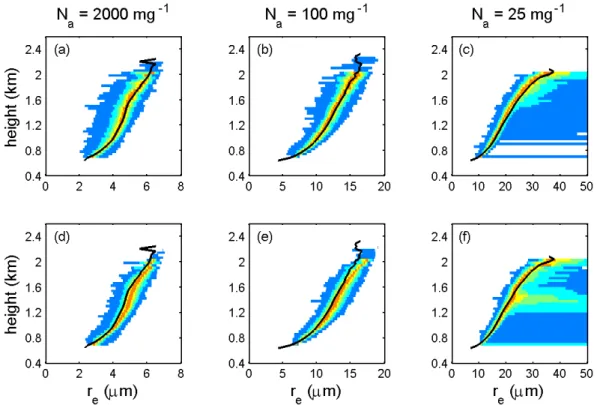
Figure 2 shows the constructedreprofiles using different measures of cloud-topre. Results using there at one grid point below the highest grid that has ql>0.01 g kg−1 are shown in Fig. 2a–c. The constructedre profiles closely rep-resent the in-cloudre, especially in the polluted and interme-diate cases. Figure 2d–f presents constructedreprofiles with the maximumrein each column. Thereprofiles constructed in this way have a high bias (∼5 %) compared to the in-cloud
Fig. 2. Constructedreprofiles using different measures of cloud-topre.(a, b, c)Usingreat one grid point below the highest grid that has
ql>0.01 g kg−1. (d, e, f)Using maximumrein the column. Color scale is the same as Fig. 1. The 50th percentile of therefrom all cloud
samples in each case are shown for reference (black lines, same as Fig. 1).
The modeled re at the uppermost grid point is smaller than that well in cloud at the same height, partly because the model assumes homogeneous mixing. For real clouds that have both homogeneous and inhomogeneous mixing, the cloud-topreshould be closer to the in-cloudre at the same height. Thus the bias in profiling the in-cloudreis likely less than 10 % using the Rosenfeld and Lensky (1998) method. Another reason for the smallerreat the uppermost grid point is that the grid may be overly diluted in the model. At the cloud boundary (for example, the cloud top), the model tends to over-dilute the cloud because of the limited model resolu-tion. It is possible that an uppermost grid point of the cloud is considered as cloudy in the model, while it is only par-tially filled with cloud in reality. The modeled cloud would then have lower LWC compared to the real cloud. However, regardless of the model performance on this issue, the upper-most grid point would be more diluted as compared with the lower grid points because of the mixing process. Detailed discussion of the effect of entrainment mixing on there pro-file and its evolution will be given in Sect. 3.3.
3.2 Evolution ofreprofiles of individual clouds
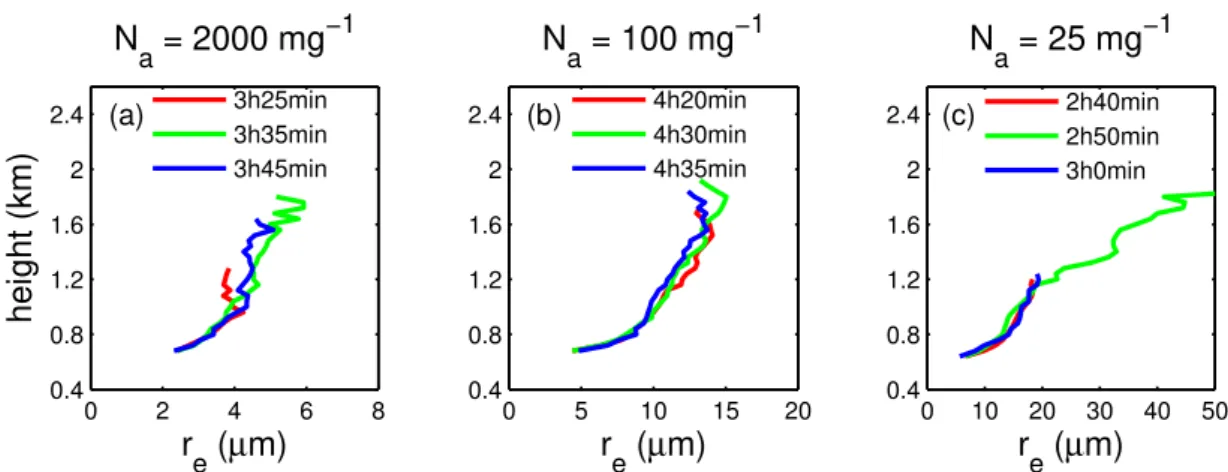
Figure 3 shows the evolution of re profiles of individual clouds at different stages of their lifetime in the simulated cases. We focus on individual clouds that are bigger but do
not merge with other clouds or break up into smaller ones throughout their lifetime. Only threere profiles during the development of each cloud are shown here. The re pro-files of an individual cloud evolving for 40 min in the pol-luted case are shown in Fig. 3a. The cloud starts to grow from 3 h 15 m, increases to the maximum height at 3 h 35 m, and completely dissipates after 3 h 55 m. It is interesting that the cloud-topre is smaller at 3 h 25 min (growing) and 3 h 45 min (decaying) compared to thereat the same heights at 3 h 35 min (growing and reaching maximum height). The reprofile at 3 h 35 min seems to fill in the cloud-topreof the lower clouds. In addition, the decaying cloud (3 h 45 min) has slightly smallerrethan the growing cloud reaching max-imum height (3 h 35 min). These characteristics ofreprofiles during cloud development may be explained by a combina-tion of the effects of precondicombina-tioning and mixing on re, as discussed in detail in Sect. 3.3.
Figure 3b shows a cloud in the intermediate case that starts to grow from 4 h 10 min and completely dissipates af-ter 4 h 35 min. It grows to its maximum height at 4 h 30 min. Similarly, thereat 4 h 30 min seems to fill in the cloud-topre of the lower clouds at the other two times. Thereof the de-caying cloud (4 h 35 min) is also slightly smaller than those of the growing clouds (4 h 20 min and 4 h 30 min).
0 2 4 6 8 0.4
0.8 1.2 1.6 2 2.4
height (km)
(a)
N
a
= 2000 mg
−1
r
e
(
µ
m)
3h25min 3h35min 3h45min
0 5 10 15 20 0.4
0.8 1.2 1.6 2 2.4 (b)
N
a
= 100 mg
−1
r
e
(
µ
m)
4h20min 4h30min 4h35min
0 10 20 30 40 50 0.4
0.8 1.2 1.6 2 2.4 (c)
N
a
= 25 mg
−1
r
e
(
µ
m)
2h40min 2h50min 3h0min
Fig. 3. Evolution ofreprofiles of individual clouds throughout their lifetime in each case.(a)A cloud in the polluted case evolving from
3 h 15 min to 3 h 55 min. The cloud reaches the maximum height at 3 h 35 min. (b)A cloud in the intermediate case from 4 h 10 min to 4 h 35 min, reaching the maximum height at 4 h 30 min.(c)A cloud in the clean case from 2 h 30 min to 3 h 5 min. It reaches the maximum height at 2 h 50 min. Only thereprofile at the time with the maximum height, and two profiles before and after the maximum height are
shown.
3 h 5 min. At 2 h 50 min, large drops form due to collision-coalescence. We can clearly see the condensation regime at a height of 0.7–1.2 km near cloud base where droplet growth is relatively slow, and the coalescence regime at the height of 1.2–1.8 km where the growth is much faster (Rosenfeld and Lensky, 1998). This confirms the findings in Figs. 1 and 2 that, for clouds that are precipitating, it is difficult to use the cloud-topreto infer the in-cloudre.
3.3 Difference ofreprofiles in growing and decaying
clouds
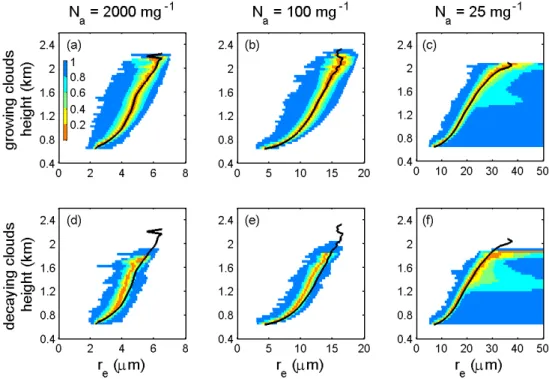
The cloud population over the last 4 h of simulation in each case is divided into growing clouds and decaying clouds based on a criterion of maximum vertical velocity. A cloud is considered as a growing (decaying) cloud if its maxi-mum vertical velocity is higher (lower) than 2 m s−1. Ide-ally a cloud that has a maximum vertical velocity smaller than 0 m s−1 might be considered a decaying cloud. How-ever, we note that using the 0 m s−1criterion leads to very few samples for decaying clouds, and that using the 1 m s−1, and 2 m s−1 criteria provides progressively more samples. The difference of re profiles in the growing and decaying clouds is very similar when using these three criteria. Fig-ure 4 shows there profiles in growing and decaying clouds using the criterion of a 2 m s−1maximum vertical velocity. The 50th percentile ofrefrom all cloud samples in each case is also shown as a reference (black lines). It is seen that, for the non-precipitating polluted and intermediate cases,re is generally smaller in the decaying clouds than in the growing clouds, probably because of progressively stronger entrain-ment mixing, as will be discussed next. In the polluted case, rein the decaying stage is about 0.5 µm smaller than that in the growing clouds. Similarly, in the intermediate case, re
in the decaying clouds is about 1 µm smaller than that in the growing clouds. The clean case has large drops in both the growing and decaying stages because large drops form due to collision-coalescence as clouds develop into mature and decaying stages.
Fig. 4. re profiles from different cloud samples in the last 4 h of simulation for the three cases. (a, b, c)Growing clouds, maximum
w >2.0 m s−1;(d, e, f)decaying clouds, maximumw <2.0 m s−1. Black lines are the 50th percentiles of therefrom all cloud samples for reference (same as in Fig. 1). Color scale is the same as Fig. 1.
concentration and a commensurately small increase inrefor marine stratocumulus clouds (Hill et al., 2008).
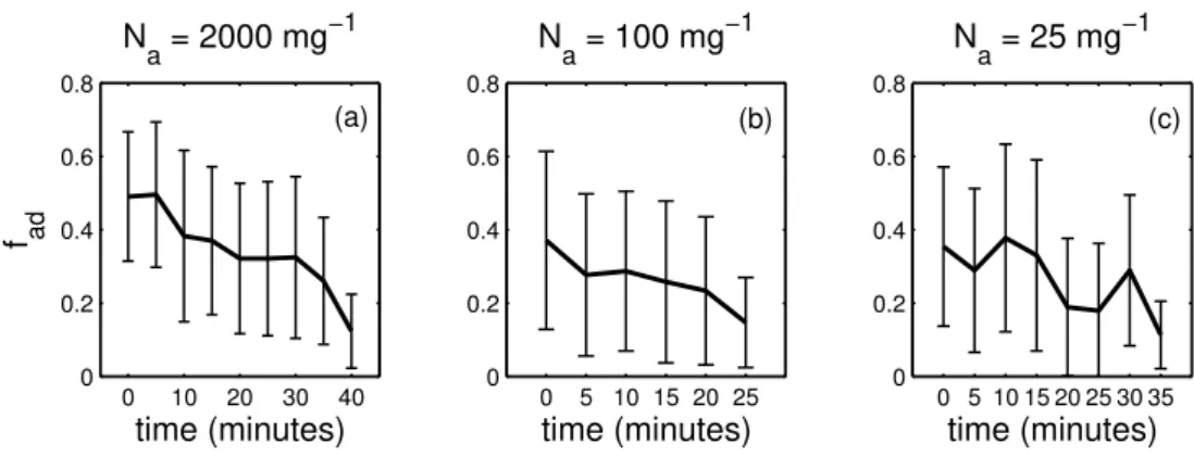
Figure 5 shows vertical profiles offadin the three simu-lated cases. It is seen thatfadis significantly smaller than 1. In the lower layer of the clouds (from cloud base to about 0.8 km), fad increases with height. Above this layer, fad generally decreases with height to about 1.6 km. Because the cloud population is dominated by clouds that are several hundred meters deep in the simulated cases, the fact thatfad decreases from 0.8 to 1.6 km indicates that liquid water mix-ing ratio in cloud samples near cloud top is reduced by en-trainment, as revealed in observations (e.g., Warner, 1955; Blyth et al., 1988; Blyth, 1993; Miles et al., 2000; Small and Chuang, 2008). The characteristics of the bigger clouds are averaged out by the smaller clouds in this layer. From 1.6 km to about 2 km, the increasedfadat cloud top in each case is due to the few bigger and deeper clouds that have higherfad. It is also likely that these larger clouds are growing in pre-conditioned, moistened air and that drops in this region are less prone to evaporation. Notice that for the polluted and intermediate cases where precipiation is negligible,fad gen-erally represents the degree of mixing. But in the clean case where precipitation develops, deviation from adiabatic liquid water content is not only affected by mixing, but also by drop sedimentation. The removal of liquid water by sedimentation is probably the reason thatfadis relatively low in the clean case compared to the other two cases.
Figure 6 shows thefadevolution of the individual clouds discussed in Fig. 3. It is seen thatfad generally decreases, representing stronger entrainment mixing, as the individual clouds grow and dissipate. The enhanced degree of mix-ing durmix-ing cloud development can cause a slight decrease inre, as can be seen in Fig. 3. It should be noted that the decrease infadis not monotonic, and shows evidence of pul-sating growth as discussed in Heus et al. (2009). Although the LES model output in this study is sampled only every 5 min, which is similar to the time scale of pulses, the non-monotonic evolution offadis consistent with the concept that a cloud can be seen as a sequence of pulses (French et al., 1999; Heus et al., 2009).
Fig. 5.Averaged profiles of adiabatic fraction (fad)over the last 4 h of simulation for the three cases. Color scale is the same as Fig. 1.
0 10 20 30 40
0 0.2 0.4 0.6 0.8
N
a = 2000 mg −1
time (minutes)
f ad
(a)
0 5 10 15 20 25
0 0.2 0.4 0.6 0.8
N
a = 100 mg −1
time (minutes) (b)
0 5 10 15 20 25 30 35 0
0.2 0.4 0.6 0.8
N
a = 25 mg −1
time (minutes) (c)
Fig. 6.Evolution offadfor the individual clouds shown in Fig. 3.
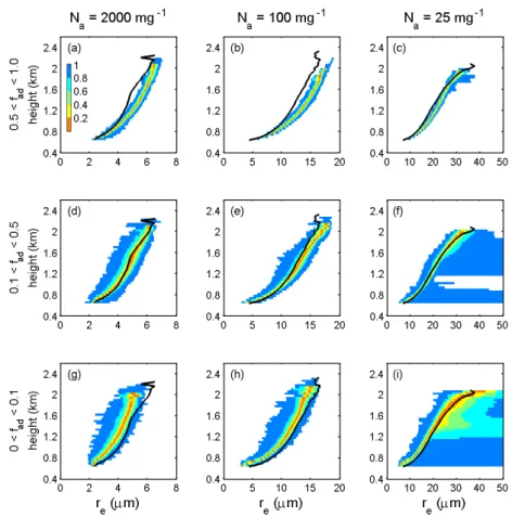
regime (0< fad<0.1) thatrehas the highest variability.rein the subadiabatic regime (0.5< fad<1.0) has small variabil-ity. For the clean, precipitating case, the strongly diluted and very strongly diluted cloud samples have drops that are much larger than the medianredue to droplet collision-coalescence and sedimentation. We do not discuss mixing effects for the clean case asfadcannot be used as an approximation for the degree of mixing in this case.
3.4 Effect of vertical inhomogeneity on shortwave radiative forcing
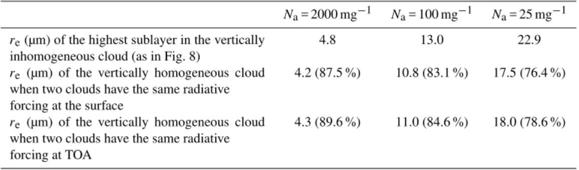
The vertical profiles of LWC andre used in the SBDART model are shown in Fig. 8. Profiles for the vertically inho-mogeneous clouds are based on the LES simulations. The LWC of the vertically homogeneous cloud is chosen in the way that the two clouds have the same LWP. We vary the reof the vertically homogeneous cloud until the two clouds have the same radiative forcing. There of the vertically ho-mogeneous cloud, along with the cloud-topre of the verti-cally inhomogeneous cloud (as in Fig. 8), are listed in Ta-ble 1. Shortwave radiative forcing both at the surface and at TOA are investigated. It is seen that thereof the vertically homogeneous cloud must be about 76–90 % of there at the
top of the vertically inhomogeneous cloud in order for them to have the same shortwave radiative forcing. The smaller values (∼76 %) are associated with clean clouds that exhibit
large vertical variation inrewhile the larger values (∼90 %)
are for polluted clouds with small vertical variation inre. Re-sults in this study are consistent with previous findings on stratified clouds (Brenguier et al., 2003).
4 Conclusions
Fig. 7. reprofiles from different cloud samples over the last 4 h of simulation for the three cases. (a, b, c)Sub-adiabatic regime (0.5<
fad<1.0);(d, e, f)strongly diluted regime (0.1< fad<0.5);(g, h, i)very strongly diluted regime (0< fad<0.1). Black lines are the 50th
percentiles of therefrom all cloud samples for reference (same as in Fig. 1). Color scale is the same as Fig. 1.
0 0.2 0.4 0.6 0.4
0.8 1.2 1.6 (a)
LWC(g m−3)
height(km)
Na=2000mg−1
2 3 4 5 0.4
0.8 1.2 1.6
re(µm)
height(km)
(d)
0 0.2 0.4 0.6 0.4
0.8 1.2 1.6
LWC(g m−3)
Na=100mg−1
(b)
5 10 15 0.4
0.8 1.2 1.6
re(µm) (e)
0 0.2 0.4 0.6 0.4
0.8 1.2 1.6
LWC(g m−3)
Na=25mg−1
(c)
5 10 15 20 25 0.4
0.8 1.2 1.6
re(µm) (f)
Fig. 8. (a, b, c)Idealized LWC profiles and(d, e, f)idealizedreprofiles for the input of the SBDART model. Black lines: LES model
results. Red lines: vertically inhomogeneous clouds that have 5 sublayers covering the height rangez= 600–1600 m; profiles are based on LES simulations. Blue lines: vertically homogeneous clouds. Note that the two clouds have the same LWP. We vary thereof the vertically
Table 1.Comparison of thereof the vertically inhomogeneous cloud with that of the vertically homogeneous cloud when two clouds have
the same shortwave radiative forcing. Numbers in parentheses represent the ratio of the two. Solar zenith angle is 60 degree.
Na= 2000 mg−1 Na= 100 mg−1 Na= 25 mg−1
re(µm) of the highest sublayer in the vertically
inhomogeneous cloud (as in Fig. 8)
4.8 13.0 22.9
re (µm) of the vertically homogeneous cloud
when two clouds have the same radiative forcing at the surface
4.2 (87.5 %) 10.8 (83.1 %) 17.5 (76.4 %)
re (µm) of the vertically homogeneous cloud
when two clouds have the same radiative forcing at TOA
4.3 (89.6 %) 11.0 (84.6 %) 18.0 (78.6 %)
is confirmed for the modeled shallow convective clouds in this study. This suggests that the cloud-topremeasured from satellites can be used to represent the in-cloudreat the same height with a low bias (about 10 %) for cumulus clouds that have negligible precipitation. The 10 % low bias is caused by the model assumption of homogeneous mixing, and also by the overly-diluted cloud edges due to model resolution. However, a caveat here is that the cloud sizes would have to fill a remote sensing pixel for these techniques to be use-ful. In addition, in reality the accuracy would be diminished by instrument and other measurement uncertainties. For the clean case where drizzle develops,reprofiles are complicated due to droplet collision-coalescence and sedimentation, and hence more difficult to characterize. The constructedre pro-files in the clean case cannot be used to represent the in-cloud reprofiles because both the in-cloudre and the constructed reare highly variable.
This study shows that the ability to distinguish a cloud under a clean aerosol condition from that under a polluted aerosol condition using both the in-cloud re and the con-structed re is good, provided the range of aerosol concen-tration is high and that the satellite retrieval ofre is robust. But for relatively small aerosol concentration gradients, the variability ofrewill make it difficult to do so.
Investigation ofreevolution for individual clouds and the cloud population indicates that re becomes smaller (about 10 %) as the cloud develops into the decaying stage. The subadiabatic characteristics of the simulated cases are inves-tigated. The adiabatic fractionfad is significantly less than 1 at all heights for the three cases, with the cloud top hav-ing smallerfad, due to stronger entrainment mixing. In ad-dition,fad becomes smaller as clouds develop into the de-caying stage. The stronger mixing at cloud top and in the decaying stage of the clouds leads to smallerre. This is the reason why the constructedreprofiles have a low bias com-pared to the in-cloudre, and decaying clouds have smallerre than the growing clouds. Results in this paper show thatre becomes progressively smaller and the variability ofrealso becomes progressively larger asfaddecreases in the polluted
and intermediate cases. It should be noted thatfadprofiles of the smaller and shallower cumulus clouds as investigated in this study may differ from those in larger and deeper clouds. For example, the core regions of deeper clouds may be able to preserve adiabatic LWC. In addition, the mixing in real-ity is probably not extremely homogeneous as assumed in the model in this study. For the cores of bigger and thicker clouds that have largerfad, and for clouds that have mogeneous mixing (or have both homogeneous and inho-mogeneous mixing), the bias in estimating the in-cloud re is likely less than 10 % using the method in Rosenfeld and Lensky (1998). However, for the clean, precipitating case, fad cannot be used to represent the degree of mixing, be-cause both entrainment mixing and sedimentation affect the distribution of liquid water.
For a vertically homogeneous cloud and a vertically in-homogeneous cloud with the same LWP,reof the vertically homogeneous cloud must be about 76–90 % of the cloud-top re of the vertically inhomogeneous cloud in order to have the same shortwave radiative forcing. This result for cumu-lus clouds is consistent with previous studies on stratiform clouds, and indicates that the estimation of cloud shortwave radiative forcing using measured cloud-top re needs to be treated carefully.
Acknowledgements. This study was supported by Chinese NSF
grant 40675004. GF acknowledges support from NOAA’s Climate Goal Program.
Edited by: J. Quaas
References
Albrecht, B.: Aerosols, cloud microphysics, and fractional cloudi-ness, Science, 245, 1227–1230, 1989.
Arakawa, A. and Schubert, W. H.: Interaction of a cumulus cloud ensemble with large-scale environment, Part one, J. Atmos. Sci., 31, 674–701, 1974.
Blyth, A. M.: Entrainment in cumulus clouds, J. Appl. Meteorol., 32, 626–641, 1993.
Blyth, A. M., Cooper, W. A., and Jensen, J. B.: A study of the source of entrained air in Montana cumuli, J. Atmos. Sci., 45, 3944–3964, 1988.
Breon, F.-M., Tanre, D., and Generoso, S.: Aeorsol effect on cloud droplet size monitored from satellite, Science, 295, 834–838, 2002.
Brenguier, J.-L., Pawlowska, H., Sch¨uller, L., Preusker, R., Fis-cher, J., and Fouquart, Y.: Radiative properties of boundary layer clouds: Droplet effective radius versus number concentration, J. Atmos. Sci., 57, 803–821, 2000.
Brenguier, J.-L., Pawlowska, H., and Sch¨uller, L.: Cloud micro-physical and radiative properties for parameterization and satel-lite monitoring of the indirect effect of aerosol on climate, J. Geo-phys. Res, 108(D15), 8632, doi:10.1029/2002JD002682, 2003. Burnet, F. and Brenguier, J.-L.: Observational study of the
entrainment-mixing process in warm convective clouds, J. At-mos. Sci., 64, 1995–2011, 2007.
Chang, F.-L. and Li, Z.: Estimating the vertical variation of cloud droplet effective radius using multispectral near-infrared satellite measurements, J. Geophys. Res., 107(D15), doi:10.1029/2001JD000766, 2002.
Chen, R., Wood, R., Li, Z., Ferraro, R., and Chang, F.-L.: Study-ing the vertical variation of cloud droplet effective radius usStudy-ing ship and space-borne remote sensing data, J. Geophys. Res., 113, D00A02, doi:10.1029/2007JD009596, 2008.
Feingold, G.: Modeling of the first indirect effect: Analysis of measurement requirements, Geophys. Res. Lett., 30, 1997, doi:10.1029/2003GL017967, 2003.
Feingold, G., Remer, L. A., Ramaprasad, J., and Kaufman, Y. J.: Analysis of smoke impact on clouds in Brazilian biomass burn-ing regions: An extension of Twomey’s approach, J. Geophys. Res., 106(D19), 22907–22922, 2001.
Feingold, G., Eberhard, W. L., Veron, D. E., and Previdi, M.: First measurements of the Twomey indirect effect using ground-based remote sensors, Geophys. Res. Lett., 30, 1287, doi:10.1029/2002GL016633, 2003.
French, J. R., Vali, G., and Kelly, R. D.: Evolution of small cumu-lus clouds in Florida: Observations of pulsating growth, Atmos. Res., 52, 143–165, 1999.
Freud, E., Rosenfeld, D., Andreae, M. O., Costa, A. A., and Ar-taxo, P.: Robust relations between CCN and the vertical evolu-tion of cloud drop size distribuevolu-tion in deep convective clouds, At-mos. Chem. Phys., 8, 1661–1675, doi:10.5194/acp-8-1661-2008, 2008.
Frisch, A. S., Fairall, C. W., and Snider, J. B.: Measurement of stratus cloud and drizzle parameters in ASTEX with a Ka-band Doppler radar and a microwave radiometer, J. Atmos. Sci., 52, 2788–2799, 1995.
Heus, T., Jonker, H. J. J., Van den Akker, H. E. A., Grif-fith, E. J., Koutek, M., and Post, F. H.: A statistical ap-proach to the life cycle analysis of cumulus clouds selected in a virtual reality environment, J. Geophys. Res., 114, D06208, doi:10.1029/2008JD010917, 2009.
Hill, A. A., Feingold, G., and Jiang, H.: The influence of
entrain-ment and mixing assumption on aerosol-cloud interactions in marine stratocumulus, J. Atmos. Sci., 66, 1450–1464, 2008. Hudson, J. G. and Yum, S. S.: Maritime-continental drizzle
con-trasts in small cumuli, J. Atmos. Sci., 58, 915–926, 2001. Jeffery, C. A. and Reisner, J. M.: A study of cloud mixing and
evolution using PDF methods. Part one: cloud front propagation and evaporation, J. Atmos. Sci., 63, 2848–2864, 2006.
Jiang, H., Feingold, G., Jonsson, H. H., Lu, M.-L., Chuang, P. Y., Flagan, R. C., and Seinfeld, J. H.: Statistical comparison of prop-erties of simulated and observed cumulus cloud in the vicinity of Houston during the Gulf of Mexico Atmospheric Composition and Climate Study (GoMACCS), J. Geophys. Res., 113, D13205, doi:10.1029/2007JD009304, 2008.
Lehmann, K., Seibert, H., and Shaw, R. A.: Homogeneous and in-homogeneous mixing in cumulus clouds: dependence on local turbulence structure, J. Atmos. Sci., 66, 3641–3659, 2009. Lensky, I. M. and Rosenfeld, D.: Satellite-based insights into
pre-cipitation formation processes in continental and maritime con-vective clouds at nighttime, J. Appl. Meteorol., 42, 1227–1233, 2003.
Lensky, I. M. and Rosenfeld, D.: The time-space exchangeabil-ity of satellite retrieved relations between cloud top temperature and particle effective radius, Atmos. Chem. Phys., 6, 2887–2894, doi:10.5194/acp-6-2887-2006, 2006.
Lohmann, U. and Feichter, J.: Global indirect aerosol effects: a re-view, Atmos. Chem. Phys., 5, 715–737, doi:10.5194/acp-5-715-2005, 2005.
Lu, M.-L., Feingold, G., Jonsson, H. H., Chuang, P. Y., Gates, H., Flagan, R. C., and Seinfeld, J. H.: Aerosol-cloud relationships in continental shallow cumulus, J. Geophys. Res., 113, D15201, doi:10.1029/2007JD009354, 2008.
McComiskey, A. and Feingold, G.: Quantifying error in the ra-diative forcing of the first aerosol indirect effect, Geophys. Res. Lett., 35, L02810, doi:10.1029/2007GL032667, 2008.
McComiskey, A., Feingold, G., Frisch, A. S., Turner, D. D., Miller, M. A., Chiu, J. C., Min, Q., and Ogren, J. A.: An assess-ment of aerosol-cloud interactions in marine stratus clouds based on surface remote sensing, J. Geophys. Res., 114, D09203, doi:10.1029/2008JD011006, 2009.
Miles, N. L., Verlinde, J., and Clothiaux, E. E.: Cloud droplet size distributions in low-level stratiform clouds, J. Atmos. Sci., 57, 295–311, 2000.
Nakajima, T. and King, M. D.: Determination of the optical thick-ness and efffecitive particel radius of clouds from reflected solar radiation measurements, Part one: Theory, J. Atmos. Sci., 47, 878–1893, 1990.
Nakajima, T., Suzuki, Y. K., and Stephens, G. L.: Droplet growth in warm water clouds observed by the A-Train, Part 1: Sensitivity analysis of the MODIS-derived cloud droplet sizes, J. Atmos. Sci., 67, 1884–1896, 2010.
Platnick, S. and Twomey, S.: Determining the Susceptibility of Cloud Albedo to Changes in Droplet Concentration with the Ad-vanced Very High-Resolution Radiometer, J. Appl. Meteorol., 33, 334–347, 1974.
Pawlowska, H., Grabowski, W. W., and Brenguier, J.-L.: Obser-vations of the width of cloud droplet spectra in stratocumulus, Geophys. Res. Lett., 33, L19810, doi:10.1029/2006GL026841, 2006.
research and teaching software tool for plane-parallel radiative transfer in the Earth’s atmosphere, Bull. Amer. Meteorol. Soc., 79, 2101–2114, 1998.
Rosenfeld, D. and Feingold, G.: Explanation of the discrepancies among satellite observations of the aerosol indirect effects, Geo-phys., Res., Lett., 30, 1776, doi:10/1029/2003GL017684, 2003. Rosenfeld, D. and Lensky, I. M.: Satellite-based insights into
pre-cipitation formation processes in continental and maritime con-vective clouds, Bull. Am. Meteorol. Soc., 79, 2457–2476, 1998. Schuller, L., Bennartz, R., Fischer, J., and Brenguier, J.-L.: An algrithm for the retrieval of droplet number concentration and geometrical thickness of statiform marine boundary clouds ap-plied to MODIS radiometric observations, J. Appl. Meteo., 44, 28–44, 2005.
Small, J. D. and Chuang, P. Y.: New observations of precipitation initiation in warm cumulus clouds, J. Atmos. Sci., 65, 2972– 2982, 2008.
Twohy, C. H., Petters, M. D., Snider, J. R., Stevens, B., Tahnk, W., Wetzel, M., Russell, L., and Burnet, F.: Evaluation of the aerosol indirect effect in marine stratocumulus clouds: Droplet number, size, liquid water path, and radiative impact, J. Geophys., Res., 110, D08203, doi:10.1029/2004JD005116, 2005.
Twomey, S.: Pollution and the planetary albedo, Atmos. Environ., 8, 1251–1256, 1974.
Twomey, S.: The influence of pollution on the shortwave albedo of clouds, J. Atmos. Sci., 34, 1149–1152, 1977.
Wang, M. and Penner, J. E.: Aerosol indirect forcing in a global model with particle nucleation, Atmos. Chem. Phys., 9, 239–260, doi:10.5194/acp-9-239-2009, 2009.
Warner, J.: The water content of cumuliform cloud, Tellus, 7, 449– 457, 1955.
Xue, H. and Feingold, G.: Large-eddy simulations of trade wind cumuli: Investigation of aerosol indirect effects, J. Atmos. Sci., 63, 1605–1622, 2006.