The Stokes phenomenon and the Lerch zeta function

The Stokes phenomenon and the Lerch zeta function

R. B. Paris

Division of Computing and Mathematics,

University of Abertay Dundee, Dundee DD1 1HG, UK

Abstract

We examine the exponentially improved asymptotic expansion of the Lerch zeta functionL(λ, a, s) =P∞

n=0exp(2πniλ)/(n+a)s for large complex values of a, with λand s regarded as parameters. It is shown that an infinite number of subdominant exponential terms switch on across the Stokes lines arg a= ±1₂π. In addition, it is found that the transition across the upper and lower imaginary a-axes is associated, in general, with unequal scales. Numerical calculations are presented to confirm the theoretical predictions.

Mathematics Subject Classification: 11M35, 30E15, 34E05, 41A30, 41A60

Keywords: Lerch zeta function, asymptotic expansion, exponentially small expansion, Stokes phenomenon, Mellin transform method

1. Introduction

A principal result of asymptotic analysis in the last quarter century has been the interpretation of the Stokes phenomenon as the smooth appearance of an exponentially small term in compound asymptotic expansions across certain rays in the complex plane known as Stokes lines. For a wide class of functions, particularly those satisfying second-order ordinary differential equations, the functional form of the coefficient multiplying such a subdominant exponential (a Stokes multiplier) is found to possess a universal structure represented to leading order by an error function, whose argument is an appropriate variable describing the transition across the Stokes line [2].

A function not satisfying a differential equation and which does not share this simple property is the logarithm of the gamma function. In [13], Paris and Wood obtained the exponentially improved expansion of log Γ(z) and showed that it involved not one but an infinite number of subdominant exponentials e±2πikz _{(k = 1,2, . . .). These exponentials are maximally subdominant on the}

|arg z| > 1

2π to eventually combine to generate the poles of log Γ(z) on the

negative z-axis. These authors demonstrated that the Stokes multipliers as-sociated with the leading exponentials (corresponding to k = 1) undergo a smooth transition approximately described by an error function in the neigh-bourhood of arg z = ±1₂π. Subsequently, Berry [3] showed, by a sequence of increasingly delicate subtractions of optimally truncated asymptotic series, that all the subdominant exponentials switch on smoothly across the Stokes lines with the multiplier given approximately by

1 2 ±

1

2erf [(θ∓ 1 2π)

q

πk|z|], (k = 1,2, . . .) (1.1)

in the neighbourhood of θ = arg z =±1₂π, respectively; see also [12, §6.4] for a detailed summary.

An analogous refinement in the large-a asymptotics of the Hurwitz zeta function

ζ(s, a) =

∞

X

n=0

(n+a)−s (ℜ(s)>1; a6= 0,−1,−2, . . .)

was considered in [10]. Across the Stokes lines arg a=±1₂π, there is a similar appearance of an infinite number of subdominant exponentials e±2πika _{(k =}

1,2, . . .), each exponential being associated with its own Stokes multiplier. For large |a|, the Stokes multipliers associated with these exponentials also undergo a smooth, but rapid, transition in the neighbourhood of arg a =±1₂π given approximately by (1.1) with z replaced by a.

In [11], the periodic zeta function F(λ, s), given by [9, §25.13]

F(λ, s) =

∞

X

n=1

e2πniλ

ns (ℜ(s)>0, 0< λ <1; ℜ(s)>1, λ∈N), (1.2)

was discussed for complex values of the parameter λ in the upper half-plane 0 < arg λ < π. This function can be expressed in terms of the Hurwitz zeta function and, accordingly, its exponentially improved large-λ expansion also consists of an infinite number of subdominant exponentials e2πikλ _{(k =}

±1,±2, . . .). In the neighbourhood of the positive imaginary λ-axis, it is found that the exponentials with k ≥1 undergo a double Stokes phenomenon, since constituent parts of F(λ, s) are associated with two parallel Stokes lines at unit distance apart.

In this paper we consider the Lerch zeta function defined for ℜ(s) > 1, 0< λ≤1 and complex a by the series [9, Eq. (25.14.1)]

L(λ, a, s) :=

∞

X

n=0

e2πniλ

and elsewhere by analytic continuation. When λ = 1, the Lerch function reduces to ζ(s, a) and when a= 1 we have

L(λ,1, s) = e−2πiλF(λ, s). (1.4)

We shall find in the large-a asymptotics of L(λ, a, s) that there is a similar appearance of an infinite number of subdominant exponential terms in the neighbourhood of the Stokes lines arg a = ±1

2π. Each of these exponentials

is associated with its own Stokes multiplier, which undergoes a smooth, but rapid, transition in the vicinity of these rays. However, unlike the situation present withζ(s, a), it will be found that the transition across the Stokes lines in the upper and lower half-planes is, in general, associated with unequal scales. We use a Mellin-Barnes integral definition of L(λ, a, s) to first determine its large-a Poincar´e expansion and then its exponentially improved expansion as |a| → ∞ in the sector |arg a| < π. The procedure we adopt is similar to that employed in [10, 13].

2. The large-a asymptotic expansion of L(λ, a, s)

2.1. An integral representation

Let a and s be complex variables with |arg a| < π and λ a real variable satisfying 0 < λ ≤ 1. When ℜ(s) > 1, we can write the Lerch zeta function defined in (1.3) as

L(λ, a, s) = a−s+a−s

∞

X

n=1

e2πiλ

1 + n a

−s

.

Making use of the representation (see, for example, [12, p. 91])

Γ(s) (1 +x)s =

1 2πi

Z c+∞i

c−∞i Γ(u)Γ(s−u)x

−u_{du (|arg x|< π),}

where1 _{1< c <ℜ(s), we obtain after an interchange in the order of summation}

and integration

L(λ, a, s) = a−s+ a

−s

2πiΓ(s)

Z c+∞i

c−∞i Γ(u)Γ(s−u)F(λ, u)a

u_{du, (2.1)}

where F(λ, u) is the periodic zeta function defined in (1.2). When λ = 1, F(1, u) becomes the Riemann zeta function ζ(u) and the representation (2.1) reduces to that given in [10] for the Hurwitz zeta function L(1, a, s) =ζ(s, a).

1

Displacement of the integration path in (2.1) to the left over the simple pole at u= 0 (and, in the case λ = 1, atu= 1) then yields

L(λ, a, s) = ǫ(λ)a

1−s

s−1 +a

−s_{{1 +F(λ,0)}+}Z(λ, a, s)

Γ(s) , (2.2)

where ǫ(λ) = 0 or 1 according as 0< λ <1 or λ= 1 and, with the change of variable u→ −u,

Z(λ, a, s) = a

−s

2πi

Z c+∞i

c−∞i Γ(−u)Γ(u+s)F(λ,−u)a

−u_{du (0< c <1). (2.3)}

The result in (2.2) and (2.3) has been derived assuming thatℜ(s)>1; but this restriction can be relaxed to allow for ℜ(s)≤1 by suitable indentation of the integration path to lie to the right of all the poles of Γ(s+u) (provided s 6=−1,−2, . . .). The representation (2.2) is similar to, but not identical with, that given in [6].

2.2. The Poincar´e asymptotic expansion

The large-a asymptotic expansion of L(λ, a, s) can be obtained by further displacement of the integration path in (2.3) over the poles of Γ(−u) at u = 1,2, . . . , K −1, where K denotes an arbitrary positive integer. This yields, when 0< λ <1,

L(λ, a, s) =a−s+

K−1

X

k=0

(−)k

k! (s)kF(λ,−k)a

−s−k_+R

K(λ, a, s), (2.4)

where (a)k = Γ(a+k)/Γ(a) is Pochhammer’s symbol. In Appendix A it is

shown that the remainder RK(λ, a, s) = O(a−s−K) as|a| → ∞ in|arg a|< π.

This expansion agrees with that given by Ferreira and L´opez [5, Thm 1], who expressed their coefficients in terms of the polylogarithm function Li−n(e2πiλ) =

F(λ,−n).

In [1], it is shown thatF(λ,−k) is expressible in terms of a certain kind of generalised Bernoulli polynomials ˜Bn(α, β) defined by the generating function

teαt

1−βet =

∞

X

n=0

˜

Bn(α, β)

n! t

n

in a neighbourhood of t = 0. From (1.4) and [1, p. 164], we have for non-negative integer values of k

F(λ,−k) = e2πiλL(λ,1,−k) = e

2πiλ

k+ 1 B˜k+1(1, e

2πiλ_{), (2.5)}

where ˜Bn(1, x) may be expressed in the form

˜

Bn(1, x) =

nPn(x)

with P1(x) = 1 and forn ≥2 thePn(x) are polynomials of degreen−2. From

[1, Eq. (3.7)], we have that

Pn(x) = n−1

X

r=1

r!S(nr−1) xr−1(1−x)n−r−1 (n≥2)

where S(r)

n are the Stirling numbers of the second kind. The first few Pn(x)

are consequently:

P2(x) = 1, P3(x) = 1 +x, P4(x) = 1 + 4x+x2,

P5(x) = 1 + 11x+ 11x2+x3, P6(x) = 1 + 26x+ 66x2 + 26x3+x4,

P7(x) = 1 + 57x+ 302x2+ 302x3 + 57x4+x5,

P8(x) = 1 + 120x+ 1191x2+ 2416x3+ 1191x4+ 120x5+x6, . . . .

Then we have the expansion given in the following theorem.

Theorem 1. Let s (6= 0,−1−2, . . .) be a complex variable and K be an arbi-trary positive integer. Then, when 0< λ < 1, we have

L(λ, a, s) = a

−s

1−e2πiλ+e

2πiλKX−1

k=1

(−)k_(s) k

k!

Pk+1(e2πiλ)a−s−k

(1−e2πiλ₎k+1 +O(a

−s−K_{) (2.7)}

as |a| → ∞ in the sector |arg a| < π.

It is worth remarking that the first few coefficients of the expansion (2.7) can be expressed in an alternative trigonometric form to yield

L(λ, a, s)

∼ a

−s

2 sinπλ

ie−πiλ+ s 2asinπλ−

is(s+ 1) cosπλ 4a2_sin2_πλ −

s(s+ 1)(s+ 2)(1 + 2 cos2_πλ)

23a3_sin3_πλ

+is(s+ 1)(s+ 2)(s+ 3)(2 + cos

2_{πλ) cosπλ}

48a4_sin4_πλ +· · ·

.

Whenλ= 1, we haveF(λ,−k) =ζ(−k) in (2.4). Then, from (2.2) and the fact that ζ(0) =−1

2, ζ(−2k) = 0 and ζ(−2k+ 1) =−B2k/(2k) (k= 1,2, . . .),

whereB2kdenote the even-order Bernoulli numbers, we recover the well-known

asymptotic expansion [7, p. 25]

L(1, a, s)≡ζ(s, a)∼ 1 2a

−s₊ a1−s

s−1 + 1 Γ(s)

∞

X

k=1

B2k

(2k)!

Γ(2k+s−1) a2k+s−1

3. The exponentially improved expansion of L(λ, a, s)

Let 0 < λ ≤ 1 and define λ′ _{:= 1 −λ. To determine the exponentially}

improved expansion of L(λ, a, s) for large|a|in|arg a|< πand, in particular, the behaviour in the neighbourhood of the rays arg a = ±1₂π, we start with the representation in (2.2), namely

L(λ, a, s) = ǫ(λ)a

1−s

s−1 +a

−s_{{1 +F(λ,0)}+}Z(λ, a, s)

Γ(s) , (3.1)

where from (2.5) and (2.6), we have F(λ,0) =e2πiλ_/(1−e2πiλ_{) when 0 < λ <1}

and F(1,0) =−1₂. The function Z(λ, a, s) is defined by the integral in (2.3).

3.1. An expansion for Z(λ, a, s)

The functional equation for the periodic zeta function F(λ, s) can be obtained from the analogous result for L(λ, a, s) given in [4, pp. 26, 29] and takes the form

F(λ, s) = Γ(1−s) (2π)s

e12πi(1−s)

∞

X

k=0

(k+λ)s−1+e−12πi(1−s)

∞

X

k=0

′_(k+λ′₎s−1 _(3.2)

for ℜ(s) < 0, where the prime on the second summation sign indicates that the term corresponding tok = 0 is to be omitted ifλ= 1. Substitution of this last result into (2.3) yields

Z(λ, a, s) = a

−s

2πi

Z c+∞i

c−∞i Γ(−u)Γ(u+s)F(λ,−u)a

−u_du

=−a

−s

4π

Z c+∞i

c−∞i

Γ(u+s) sinπu (2πa)

−u

×

e12πiu

∞

X

k=0

(k+λ)−1−u−e−12πiu

∞

X

k=0

′_(k+λ′₎−1−u_du,

where 0< c <1. We define the sum

E(λ, s;z) :=

∞

X

k=0

(k+λ)s−1Jk(λ, s;z), (3.3)

where

Jk(λ, s;z) :=

1 4π

Z c+∞i

c−∞i

Γ(u+s) sinπu z

−u−s_{du (0< c <1, |arg z|<} 3 2π).

(3.4) Then we obtain

Z(λ, a, s) = (2π)s{e12πisE(λ′, s;iX′)−e− 1

where

X := 2πa(k+λ), X′ := 2πa(k+λ′) (3.6) and in the sum E(λ′_{, s;iX}′_{) the term corresponding tok = 0 is understood to}

be omitted if λ= 1.

We now displace the (possibly indented whenℜ(s)≤0) integration path for Jk(λ, s;−iX) in (3.4) to the right over the poles situated atu= 1,2, . . . , Nk−1,

where the {Nk} (k ≥ 1) denote (for the moment) an arbitrary set of positive

integers. This produces

Jk(λ, s;−iX) =

1 2πi

Nk−1

X

r=1

(−)rΓ(r+s)(−iX)−r−s+Rk(λ, a;Nk), (3.7)

where the remainder term is given by

Rk(λ, a;Nk) =

1 4π

Z −c′+Nk+∞i

−c′_+Nk−∞i

Γ(u+s)

sinπu (−iX)

−u−s_du

= (−)

Nk

4π

Z −c′+∞i

−c′_−∞i

Γ(u+νk)

sinπu (−iX)

−u−νk

du, (3.8)

with 0< c′ _{<1. In the last integral, we have replaced the integration variable}

u by u+Nk and have set

νk :=Nk+s.

It is also tacitly assumed that ℜ(νk)−c′ > 0 so that the integration path in

Rk(λ, a;Nk) is not indented when ℜ(s)≤0.

The integrals in (3.8) can be identified in terms of the so-called terminant function (see [9, p. 67]), which is a multiple of the incomplete gamma function Γ(a, z) (or, equivalently, the exponential integral). Following the notation employed in [12, p. 243], we denote the terminant function by Tν(z), where

Tν(z) = eπiν

Γ(ν)

2πi Γ(1−ν, z)

= e

−z

4π

Z −c+∞i

−c−∞i

Γ(u+ν) sinπu z

−u−ν_{du (|arg z|<} 3

2π), (3.9)

where 0< c < 1 and, provided ν 6= 0,−1,−2, . . ., the integration path lies to the right of all the poles of Γ(u+ν); see [9, p. 178]. It then follows from (3.8) that

Rk(λ, a;Nk) =e−iX−πisTνk(−iX) (|arg a|< π). (3.10) Proceeding in the same manner for the integralJk(λ′, s;iX′), with the set of

integers {Nk}replaced by the set {Nk′}and the parameters νk byνk′ :=Nk′+s,

we find

Jk(λ′, s;iX′) =

1 2πi

N′

k−1

X

r=1

(−)r_Γ(r+s)(iX′₎−r−s_+R′

where

R′_k(λ′, a;N_k′) =eiX′−πisTν′

k(iX

′_{) (|arg a|< π). (3.12)}

Then, from (3.5), we finally obtain

Z(λ, a, s) (2π)s =

∞

X

k=0

(k+λ)s−1

i

2π

Nk−1

X

r=1

(−i)r_Γ(r+s)

Xr+s −e

−1 2πisR

k(λ, a;Nk)

−

∞

X

k=0

′_(k+λ′₎s−1 i

2π

N′

k−1

X

r=1

ir_Γ(r+s)

X′r+s −e

1 2πisR′

k(λ′, a;Nk′)

(3.13)

valid in |arg a|< π.

When λ= 1, we have X =X′ _{= 2πika and N}

k=Nk′. The right-hand side

of (3.13) then reduces to

∞

X

k=1

ks−1

1

π

nk−1

X

r=0

(−)rΓ(2r+s+ 1)

X2r+s+1 +Rk(a;nk)

,

where the {nk}denote an arbitrary set of positive integers and

Rk(a;nk) =e−πis{eiX+

1 2πisT

νk(iX)−e −iX−1

2πisT

νk(−iX)}, νk := 2nk+s as found in [10, Eq. (2.5), (2.6)] for the Hurwitz zeta function ζ(s, a).

Assuming that Nk < Nk+1, Nk′ < Nk′+1 (k = 0,1,2, . . .), we can write the

double sum involving λ in (3.13) in the form [3], [12,§6.4.3]

∞

X

k=0

(k+λ)s−1

Nk−1

X

r=0

(−i)r_Γ(r+s)

Xr+s =

∞

X

k=0

Nk−1

X

r=0

(−i)r_Γ(r+s)

(2πa)r+s_(k+λ)r+1

=

∞

X

m=0

Nm−1

X

r=Nm₋1

(−i)r_Γ(r+s)

(2πa)r+s ζ(r+1, m+λ),(3.14)

where the sum over k has been evaluated in terms of the Hurwitz zeta function and N−1 = 1; see Appendix B for details. A similar rearrangement applies to

the other double sum in (3.13) involving λ′ _{(with N}′

−1 = 1).

If we define

Hm(a;λ, λ′) := Nm−1

X

r=Nm₋1

(−i)r_Γ(r+s)

(2πa)r+s ζ(r+ 1, m+λ)

−

N′

m−1

X

r=N′

m₋1

ir_Γ(r+s)

(2πa)r+s ζ(r+ 1, m+λ

′_{), (3.15)}

Theorem 2. Let λ′ _{= 1−λ, ǫ(λ) = 0 or 1 according as 0< λ <1 or λ= 1.}

Let the truncation indices Nk and Nk′ be increasing sets of positive integers

with νk = Nk+s, νk′ = Nk′ +s. Then, for 0< λ ≤ 1, we have the expansion

of L(λ, a, s) given by

L(λ, a, s) = ǫ(λ)a

1−s

s−1 +a

−s_{1+F(λ,0)}+(2π)s

Γ(s)

∞

X

m=0 ′ i

2π Hm(a;λ, λ

′₎

− e

−1 2πis

(m+λ)1−sRm(λ, a;Nm) +

e12πis (m+λ′₎1−s R

′

m(λ′, a;Nm′ )

(3.16)

valid in |arg a|< π, where

Rm(λ, a;Nm) =e−iX−πisTνm(−iX), R ′

m(λ′, a;Nm′ ) =eiX ′_−πis

Tν_m′ (iX′)

and X, X′ _{are defined in (3.6). The prime on the summation sign indicates}

that the terms corresponding to m = 0 in the sums involving λ′ _{are to be}

omitted when λ= 1.

3.2. The optimally truncated expansion and the Stokes multipliers

An important feature of (3.13) is that the Poincar´e expansion in (2.7) has been decomposed into two k-sequences of component asymptotic series with scales 2πa(k+λ) and 2πa(k+λ′_{), each associated with its ownarbitrary truncation}

index Nk and Nk′ and remainder terms Rk(λ, a;Nk) and Rk′(λ′, a;Nk′). From

the large-argument asymptotics of the incomplete gamma function [9, p. 179]

Γ(a, z)∼za−1e−z (|z| → ∞, |arg z|< 3 2π)

and the first equation in (3.9), the sums involving the remainders are abso-lutely convergent, since the decay of the late terms is controlled byk−Nk−1and k−N′

k−1. It then follows that the result in (3.13) is exact and that no further expansion process is required.

The infinite sequences of exponentials e2πia(k+λ) _{and e}−2πia(k+λ′₎

for non-negative integer k are seen to emerge from the remainders in (3.13), or (3.16), with the terminant functions Tνk(−iX) and Tν′_k(iX

′_{), respectively, as}

coeffi-cients. These exponentials are maximally subdominant on the negative and positive imaginary axes, respectively and steadily increase in magnitude as one approaches the negative reala-axis where they eventually combine to generate the singularities of L(λ, a, s) at negative integer values of a.

If the truncation indices Nk and Nk′ are now chosen to correspond to the

optimal truncation values (i.e., truncation at or near the least term in the corresponding inner series over r in (3.13)), then it is easily shown that

In this case, νk =|X|+O(1), νk′ =|X′|+O(1) and we see that the order and

the argument of each terminant function appearing in (3.13) are approximately equal in the limit |a| → ∞. When |ν| ∼ |z| ≫1, the function Tν(z) possesses

the asymptotic behaviour [8], [12, §6.2.6]

Tν(z) ∼             

−ie(π−φ)iν

1 +e−iφ

e−z−|z|

q

2π|z|{1 +O(z

−1_{)} −π+δ≤φ≤π−δ}

1 2 +

1

2erf [c(φ)( 1 2|z|)

1

2] +O(z− 1 2e−

1 2|z|c

2

(φ)_{), δ ≤φ ≤2π−δ}

(3.18) where φ = arg z, δ denotes an arbitrarily small positive quantity and c(φ) is defined implicitly by

1 2c

2_{(φ) = 1 +i(φ−π)−e}i(φ−π)

with the branch for c(φ) chosen so that c(φ) ≃ φ − π near φ = π. Thus, the function Tν(z) changes rapidly, but smoothly, from being exponentially

small in |arg z| < π to having the approximate value unity as arg z passes continuously through π.

The result in (3.13) and (3.16), when the truncation indices Nk and Nk′

are chosen according to (3.17), then constitutes the exponentially improved expansion of L(λ, a, s). For fixed, large |a| in the vicinity of arg a = 1

2π,

the dominant contribution to the remainder arises from the term involving Tν′

k(iX

′_{), the other remainder involving T}

νk(−iX) being smaller. The coeffi-cient of each subdominant exponential exp (2πi(k+λ′_{)a) then has the leading}

behaviour from (3.18) given by

e−12πisT

ν′

k(iX

′_)∼e−1 2πis{1

2 + 1

2erf [c(θ− 1 2π)

q

π(k+λ′_)|a|]},

where θ = arg a and, near θ = 1₂π, the quantity c(θ− 1₂π)≃ θ− 1₂π. In the vicinity of arg a = −1

2π, the role of the two remainders is reversed and the

coefficient of each subdominant exponential exp (−2πi(k+λ)a) becomes

−e−32πisT

νk(−iX) = e 1

2πis(1−T

νk(Xe 3

2πi)) (3.19)

≃ e12πis{1

2 − 1

2erf [c(θ+ 1 2π)

q

π(k+λ)|a|]},

where we have made use of the connection formula for Tν(z) given by [12,

Eq. (6.2.45)]

Tν(ze−πi) =e2πiν{Tν(zeπi)−1}. (3.20)

The approximate functional form of the Stokes multiplier for L(λ, a, s) (excluding the factors e∓1

2πis/Γ(s)) in the vicinity of arg a=±1

2π is therefore

found to be

1 2 ±

1

2erf [(θ∓ 1 2π)

q

respectively, where ξ = λ′ _{near arg a =} 1

2π and ξ = λ near arg a = − 1 2π.

When λ = 1, ξ ≡ 0 and the form (3.21) then applies to the Hurwitz zeta functionζ(s, a) withk = 1,2, . . .; see [10, Section 3]. The approximation (3.21) describes the birth of each subdominant exponential in the neighbourhood of the positive and negative imaginary axes on the increasingly sharp scale (π(k + ξ)|a|)1/2_{. It is immediately apparent that the transition across the}

Stokes lines is associated withunequal scales in the upper and lower half-planes, except when λ = 1₂ (where the function L(1₂, a, s) reduces to the alternating variant of the Hurwitz zeta function).

4. Numerical results

In order to display numerically the smooth appearance of thenth subdominant exponential e2πi(n+λ′_)a

in the vicinity of arg a = 1₂π (at fixed |a|), it is neces-sary to ‘peel off’ from Z(λ, a, s) the larger subdominant exponentials in the remainder terms and all larger terms of the asymptotic series in (3.13). This has been carried out in the expansion in (3.16) by means of the rearrangement in (3.14)

We define thenth Stokes multiplier Sn(θ) (withθ= arg a) associated with

the exponential e2πi(n+λ′_)a

in the vicinity of arg a = 1₂π by subtracting from Z(λ, s, a)/(2π)s_{the asymptotic seriesH}

m(a;λ, λ′) corresponding to 0≤m≤n

and the larger subdominant exponentials 0≤m ≤n−1 in R′

m(λ′, a;Nm′ ) and

0≤m ≤n inRm(λ, a;Nm). Thus we have

Z(λ, s, a) (2π)s −

i 2π

n X

m=0

Hm(a;λ, λ′) =e

1 2πis

n−1

X

m=0

R′

m(λ′, a;Nm′ )

(m+λ′₎1−s

−e−12πis

n X

m=0

Rm(λ, a;Nm)

(m+λ)1−s +

e2πi(n+λ′)a−12πis

(n+λ′₎1−s Sn(θ).

It then follows that near arg a= 1₂π

Sn(θ) =

e−2πi(n+λ′)a+12πis (n+λ′₎1−s

Z(λ, s, a)

(2π)s −

i 2π

n X

m=0

Hm(a;λ, λ′)

−e12πis

n−1

X

m=0

R′

m(λ′, a;Nm′ )

(m+λ′₎1−s +e

−1 2πis

n X

m=0

Rm(λ, a;Nm)

(m+λ)1−s

(4.1)

for n = 0,1,2, . . ..

Similarly, near arg a = −1

2π, we write the term corresponding to m = n

in the sum involving Rm(λ, a;Nm) in (3.16) with the aid of (3.19). Then the

Stokes multiplier near arg a =−1₂π is defined by

Sn(θ) =

e2πi(n+λ)a−1 2πis

(n+λ)1−s

Z(λ, s, a)

(2π)s −

i 2π

n X

m=0

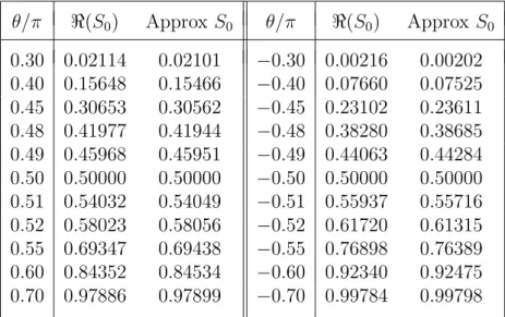
Table 1: The real part of the Stokes multiplierS0(θ) fora= 5e

iθ

whens= 4 andλ= 2/3 compared with the approximate value (3.21) with k = 0. The optimal truncation indices areN0= 17,N0′ = 7.

θ/π ℜ(S0) Approx S0 θ/π ℜ(S0) Approx S0

0.30 0.02114 0.02101 −0.30 0.00216 0.00202 0.40 0.15648 0.15466 −0.40 0.07660 0.07525 0.45 0.30653 0.30562 −0.45 0.23102 0.23611 0.48 0.41977 0.41944 −0.48 0.38280 0.38685 0.49 0.45968 0.45951 −0.49 0.44063 0.44284 0.50 0.50000 0.50000 −0.50 0.50000 0.50000 0.51 0.54032 0.54049 −0.51 0.55937 0.55716 0.52 0.58023 0.58056 −0.52 0.61720 0.61315 0.55 0.69347 0.69438 −0.55 0.76898 0.76389 0.60 0.84352 0.84534 −0.60 0.92340 0.92475 0.70 0.97886 0.97899 −0.70 0.99784 0.99798

−e12πis

n X

m=0

R′

m(λ′, a;Nm′ )

(m+λ′₎1−s +e

−1 2πis

n−1

X

m=0

Rm(λ, a;Nm)

(m+λ)1−s

(4.2)

for n = 0,1,2, . . ..

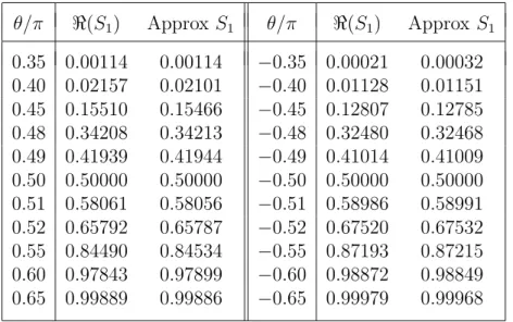
In Tables 1 and 2 we show the real part2 _{of S}

n(θ) for n = 0 and 1

com-puted from (4.1) and (4.2) compared with the approximate value in (3.21) when a = 5eiθ _{and s = 4, λ =} 2

3 as a function of θ in the vicinity of the

positive and negative imaginary a-axes. In the computation ofSn(θ) it is

nec-essary to compute the terms Rm(λ, a;Nm) and R′m(λ′, a;Nm′ ) by means of the

incomplete gamma function representation in (3.9) and the sum Hm(a;λ, λ′)

to the required exponential accuracy. The optimal truncation indices Nk and

N′

k were obtained by inspection of the terms in the algebraic expansions. In

addition, when computing the terminant functions appearing in Rm(λ, a;Nm)

and R′

m(λ′, a;Nm′ ) one must use the connection formula (3.19) once the

argu-ment ofz inTν(z) has exceededπ, since Mathematicaonly computes the value

of the incomplete gamma function in the principal sector −π < arg z ≤π. It is seen that there is good agreement between the real part of the com-puted values of the Stokes multiplier and the predicted approximate values in (3.21). Moreover, the tables confirm that the transition scales across the positive and negative imaginary a-axes depend on λ′ _{and λ, respectively, and}

are indeed unequal (except when λ= 1₂).

2

Table 2: The real part of the Stokes multiplierS1(θ) fora= 5e

iθ

whens= 4 andλ= 2/3 compared with the approximate value (3.21) with k = 1. The optimal truncation indices areN0= 17,N0′ = 7,N1= 49,N1′ = 38.

θ/π ℜ(S1) Approx S1 θ/π ℜ(S1) Approx S1

0.35 0.00114 0.00114 −0.35 0.00021 0.00032 0.40 0.02157 0.02101 −0.40 0.01128 0.01151 0.45 0.15510 0.15466 −0.45 0.12807 0.12785 0.48 0.34208 0.34213 −0.48 0.32480 0.32468 0.49 0.41939 0.41944 −0.49 0.41014 0.41009 0.50 0.50000 0.50000 −0.50 0.50000 0.50000 0.51 0.58061 0.58056 −0.51 0.58986 0.58991 0.52 0.65792 0.65787 −0.52 0.67520 0.67532 0.55 0.84490 0.84534 −0.55 0.87193 0.87215 0.60 0.97843 0.97899 −0.60 0.98872 0.98849 0.65 0.99889 0.99886 −0.65 0.99979 0.99968

Appendix A: Estimation of the remainder RK(λ, a, s) in (2.4)

The remainder term RK(λ, a, s) in (2.4) resulting from displacement of the

integration path in (2.3) is given by

RK(λ, a, s) =

a−s

2πi

Z K−c+∞i

K−c−∞i Γ(−u)Γ(s+u)F(λ,−u)a

−u_{du (0< c <1).}

Following the procedure described in Section 3 combined with use of the func-tional equation for F(λ,−u) in (3.2), we easily obtain

RK(λ, a, s)

(2π)s =e

−1 2πis

∞

X

k=0

′_(k+λ′₎s−1_eiX′

Tν(iX′)−e−

3 2πis

∞

X

k=0

(k+λ)s−1e−iXTν(−iX),

(A.1) whereTν(z) is the terminant function in (3.9),ν =K+sandX,X′are defined

in (3.6).

Since [12, p. 260]

ezTν(z) =−ieπiν

Γ(ν)

2π U(ν, ν, z),

whereU(a, b, z) denotes the second confluent hypergeometric function [9, p. 322], it is seen that the expansion (2.4) with the remainder given in (A.1) becomes

L(λ, a, s) =a−s+

K−1

X

k=0

(−)k

k! (s)kF(λ,−k)a

−s−k_{+ (−)}K_(2π)s (s)K

×

e12πis

∞

X

k=0

(k+λ′)s−1U(ν, ν, iX′)−e−12πis

∞

X

k=0

(k+λ)s−1U(ν, ν,−iX)

(A.2) when 0 < λ < 1. This is similar to, but not identical with, the expansion obtained in [6].

For fixed ν, we have the asymptotic behaviour [9, p. 328]

U(ν, ν, z)∼z−ν (|z| → ∞, |arg z|< 3₂π).

It then follows that for fixed integer K

RK(λ, a, s)

(2π)s ∼ (2πa)

−ν Γ(ν)

2πi

e12πiK

∞

X

k=0

′_(k+λ′₎−K−1_−e−1 2πiK

∞

X

k=0

(k+λ)−K−1

= O(a−K−s) (A.3)

as |a| → ∞ in|arg a|< π, since the sums are finite and independent of a.

Appendix B: The double series rearrangement in (3.14)

The rearrangement of the double series in (3.14) follows the procedure de-scribed in [3]; see also [12, §6.4.3] for an account of this process. If we set Ar := (−i)rΓ(r+s)/(2πa)r+s, the double sum in (3.13) involving λ and the

truncation indices {Nk}(k ≥0) can be rearranged3 as

∞

X

k=0

Nk−1

X

r=1

Ar

(k+λ)r+1

=

N0−1

X

r=1

Ar

λr+1 +

N0−1

X

r=1

+

N1−1

X

r=N0

A

r

(1+λ)r+1 +

N0−1

X

r=1

+

N1−1

X

r=N0 +

N2−1

X

r=N1

A

r

(2+λ)r+1 +· · ·

=

N0−1

X r=1 Ar ∞ X k=0 1

(k+λ)r+1 +

N1−1

X

r=N0 Ar

∞

X

k=1

1

(k+λ)r+1 +

N2−1

X

r=N1 Ar

∞

X

k=2

1

(k+λ)r+1 +· · ·

=

∞

X

m=0

Nm−1

X

r=Nm₋1

Arζ(r+ 1, m+λ),

where the sums over k have been evaluated in terms of the Hurwitz zeta function and N−1 = 1. A similar result applies to the other double sum

involving λ′ _{in (3.13) with N}′ −1 = 1.

3

References

[1] T.M. Apostol, On the Lerch zeta function, Pacific J. Math.1(1951) 161–167.

[2] M.V. Berry, Uniform asymptotic smoothing of Stokes’s discontinuities, Proc. Roy. Soc. LondonA422(1989) 7–21.

[3] M.V. Berry, Infinitely many Stokes smoothings in the gamma function, Proc. Roy. Soc. LondonA434(1991) 465–472.

[4] A. Erd´elyi, W. Magnus, F. Oberhettinger and F.G. Tricomi, Higher Transcendental Functions, vol. 1, McGraw-Hill, New York, 1953.

[5] C. Ferreira and J.L. L´opez, Asymptotic expansions of the Hurwitz-Lerch zeta function, J. Math. Anal. Appl.298(2004) 210–224.

[6] M. Katsurada, Power series and asymptotic series associated with the Lerch zeta-function, Proc. Japan Acad.74A (1998) 167–170.

[7] W. Magnus, F. Oberhettinger and R.P. Soni, Formulas and Theorems for the Special Functions of Mathematical Physics, Springer, New York, 1966.

[8] F.W.J. Olver, Uniform, exponentially improved, asymptotic expansions for the gener-alized exponential integral, SIAM J. Math. Anal.22(1991) 1460–1474.

[9] F.W.J. Olver, D.W. Lozier, R.F. Boisvert and C.W. Clark,NIST Handbook of Math-ematical Functions, Cambridge University Press, Cambridge, 2010.

[10] R.B. Paris, The Stokes phenomenon associated with the Hurwitz zeta functionζ(s, a), Proc. Roy. Soc. LondonA461(2005) 297–304.

[11] R.B. Paris, The Stokes phenomenon associated with the periodic zeta functionF(a, s). arXiv:1407.2782 (2014).

[12] R.B. Paris and D. Kaminski,Asymptotics and Mellin-Barnes Integrals, Encyclopedia of Mathemetics and Its Applications, Vol. 85, Cambridge University Press, Cambridge, 2001.

[13] R.B. Paris and A.D. Wood, Exponentially improved asymptotics for the gamma func-tion, J. Comp. Appl. Math.41(1992) 135–143.