The relationships of alternative energies with the technology sector and non-renewable energies

(1)

Escola de Economia de Empresas de São Paulo

Ricardo Miguel Silva Barão

The relationships of Alternative Energies

with the Technology Sector

and non-Renewable Energies

(2)

Ricardo Miguel Silva Barão

The relationships of Alternative Energies

with the Technology Sector

and non-Renewable Energies

SÃO PAULO 2015

Dissertação apresentada à Escola de Economia de Empresas de São Paulo da

Fundação Getúlio Vargas, como

requisito para obtenção do título de Mestre Profissional em Finanças.

Campo do Conhecimento: International Master in Finance

(3)

Barão, Ricardo.

The relationships of Alternative Energies with the Technology Sector and

non-Renewable Energies / Ricardo Barão - 2015.

48 f.

Orientador: Pedro Valls.

Dissertação (mestrado) - Escola de Economia de São Paulo.

1. Energia renovável. 2. Modelos econométricos. 3. Tecnologia. 4. Investimentos. I. Valls, Pedro. II. Dissertação (mestrado) - Escola de Economia de São Paulo. III. Título.

(4)

The relationships of Alternative Energies

with the Technology Sector

and non-Renewable Energies

Dissertação apresentada à Escola de Economia de Empresas de São Paulo da

Fundação Getúlio Vargas, como

requisito para obtenção do título de Mestre Profissional em Finanças.

Campo do Conhecimento: International Master in Finance

Data de Aprovação: ___/___/____.

Banca Examinadora:

_________________________________ Prof. Dr. Pedro Valls

_________________________________ Prof. Dr. Pedro Pereira

_________________________________

(5)

Acknowledgements

I would like to first acknowledge the help of my supervisors, their insightful

observations and availability made this work possible. To Professor Doutor Pedro Valls

and Professor Doutor João Pedro Pereira, my deepest thanks.

I would also like to express my thanks to all the Professors in Lisbon, São Paulo

and London which I had the privilege of knowing and with whom I learned interesting

subjects and different ways of thinking.

To my family, without their support this task would have not been possible. I

want to deeply thank my Dad, my Mum that gave me the support I needed in all

moments of this path.

Finally to my friends, Daniel and João, that in Portugal always paid attention to

what was happening in São Paulo and during the thesis always supported me. It was

very important.

To all of you, thank you very much,

(6)

Resumo

Este trabalho tem como objectivo compreender de que forma os investidores

veem as energias renováveis: se as veem como parte do sector tecnológico, à espera de

novos desenvolvimentos, ou como uma alternativa aos métodos existentes de produção

de energia. Para responder a esta questão, foi desenvolvido um modelo de vectores

autoregressivos com quatro variáveis de forma a se poder aplicar um Granger causality

test e Impulse Response function. Os resultados sugerem que para o período de

2002-2007 à escala global ambas as hipóteses se confirmam, porém de 2009-2014 os

resultados sugerem que os investidores não reconhecem as energias renováveis como

um ramo do sector tecnológico, neste período. Para além disso, durante o período de

2009-2014, e quando comparados investidores Americanos com Europeus, os resultados

sugerem que apenas o último identifica as energias renováveis como uma fonte viável

para a produção energética.

Palavras Chave: Vector Autoregressivo, Energias Renováveis, Tecnologia,

(7)

Abstract

This work aimed to understand the investor perception on clean energy: if it is

seen as part of the technology sector, awaiting new developments, or as an alternative to

the existing energy production methods. To answer this question, a four variable vector

autoregression model was developed so that a Granger causality test and Impulse

response function could be applied. The results suggest that while both hypotheses were

confirmed worldwide for the period 2002-2007, from 2009 to 2014 results suggest that

investors do not recognize the field of clean energy as part of the technology sector.

Moreover, during the period that ranges from 2009 to 2014, and when comparing the

American investor with the European investor, only the latter identifies renewable

energy as a viable source of energy production.

Key Words: Vector autoregression, Clean energy, Technology, Non-renewable

(8)

Index of tables

Table 1 - Correlation Matrix. ... 22

Table 2 - Correlation Matrix. ... 23

Table 3 - Descriptive statistics ... 24

Table 4 - Descriptive statistics ... 25

Table 5 - Unit Roots ... 28

Table 6 - Unit Roots ... 29

Table 7 - Granger causality test ... 30

Table 8 - Granger causality test ... 30

Table A1 - Coefficients of Unrestricted VAR ... 49

Table A5 -Fit of Unrestricted VAR ... 49

Table A6 - Fit of Unrestricted VAR ... 48

Table A9 - Lagrange-multiplier test ... 49

Index of figures Figure 1 - Expected growth of primary energy demand worldwide... 10

Figure 2 - Time series plot. ... 12

Figure 3 - Impulse response function. ... 32

Figure 4 - Impulse response function ... 33

Figure 5 - Impulse response function. ... 34

Figure 6 - Impulse response function ... 35

Figure A1 - Histograms. ... 44

Figure A2 - Histograms ... 44

48 48 47 45

(9)

1. Introduction

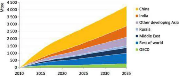
In recent years, an increase in energy demand has been observed which was

mostly driven by demand from developing countries, mainly China and India, figure 1.

While in the past, a situation as such would be overcome by a raise in the

non-renewable energies supply, the same principle cannot be applied nowadays. There are

concerns over the greenhouse effects of such energy sources. These issues together with

three other facts: 1) both developed and developing countries avoidance in needing

commodities which are sourced from areas of geopolitical tension; 2) the European “20

-20-20 program” setting European Union to have 20% of the total energy produced

coming from renewable energy by 2020; and 3) the U.S. commitment to invest in clean

energies as stated by the President Obama; are leading to an unprecedented interest in

enewable sources of energy. Nonetheless, are renewable energies already perceived as

alternatives to non-renewable energies?

(11)

In the beginning of the new millennium, renewable energies were heavily

dependent on new scientific and technological innovations in order to improve their

efficiency, reduce their costs and to be a real contender for energy production. In a

study by Sadorsky and Henriques (2008), it was demonstrated that U.S. investors

looked at alternative energy companies in a similar way as to other high technology

companies, in other words, renewable energy was not seen as an efficient technology

yet. The aim of this work project is to extend on previous studies in this area and to

understand the current perception of investors on alternative energies. Finally, an

additional aim of this project is to discern differences in investor attitudes towards clean

energy according to their geographical region. To this end, viewpoints from European

and U.S. investors were considered and also viewpoints at a worldwide scale were

studied by analysis of indexes for each region.

In order to accomplish the goals, a methodology similar to that presented by

Sadorsky and Henriques (2008) is followed, where a four variable vector autoregression

model is developed and estimated. Subsequently, a Granger causality test and an

Impulse response function are applied to study the relationship among the variables.

The variables used are: 1) an index composed by renewable energies companies; 2) an

index made of technology companies which produce some of the components used by

clean energy companies; 3) oil price, to understand the link between alternative energies

with non-renewable sources; and 4) an index of gas and oil companies. The hypothesis

behind the inclusion of the latter is can it provide insights into the differences between

renewable and non-renewable companies relationships with oil and technology.

The usage of oil price as variable instead of gas price had to do with the

following reasons. Despite of energy companies, that use non-renewable commodities

(12)

being the main output of clean energy, the inclusion of oil price in this work is justified

by a study carried out by Mohammadi (2009) where it was concluded that the gas price

is regional while the price of oil is global. This characteristic is majorly important for

the worldwide analysis as well as to the comparison between regions. Additionally,

Mohammadi (2009) proved that even though oil is scarcely used for electricity produce,

fluctuations in its price have an impact on the price of electricity.

Figure 2 shows a time series from plot of the four variables with data ranging

from 16th November 2001 to 26th May 2015 global data: the Ardour Global Alternative

Index (Renewable), the i-shares Global Energy ETF (Energy), the i-shares Global

Technology ETF (Technology) and oil prices at WTI (Oil). In order to ease the

comparison among the variables, they were normalized to 100 on the first time-point

(16th November 2001).

Figure 2 - Indexes: Oil and Gas (Energy), Renewable Energy (Renewable) and Technology (Technology); and oil price (Oil). Base year as value of 100.

0 100 200 300 400 500 600

16-11-2001 16-11-2005 16-11-2009 16-11-2013

Index

or

pri

ce

(13)

Due to the significant impact of the subprime crisis in all the variables

considered and to better understand eventual changes in the investors viewpoint before

and after the crisis, the data was split in two time periods, leaving the financial crisis

period (from October 2007 until December of 2009) out of the analysis. The period

from the 1st October 2014 onwards is also not taken into account due to the plunge in

the oil price and in the Euro/USD exchange rate. The first event has had major

implications in the relationship between the variables related to energy, while the latter

has mainly affected the European indexes.

(14)

2. Literature Review

Significant emission levels of greenhouse gases, such as carbon dioxide (CO2),

have resulted in a serious global-warming problem, which is having a tremendous

impact in the world’s climate (Cox et al., 2000). Oil consumption leads to the release of

CO2, which is understood as one of the most important contributors to climate change.

Moreover, the oil price has a huge impact in the economy of OECD members since a

10% increase in its price leads to a decrease of 0.5% in the GDP, due to a raise in

inflation and unemployment therefore affecting macroeconomic growth (Awerbuch and

Sauter, 2006). Oil price fluctuations are so impactful that numerous studies have been

conducted in the last years to further understand their effect on the stock market returns.

In particular, a study employing a Granger causality model has analyzed fluctuations in

demand, supply and idiosyncratic demand shocks of oil and concluded that only the

latter has a significant impact on stock market returns (Apergis and Miller, 2009).

Additionally, since oil is a traded commodity, its price should be governed by oil’s

global demand and supply but in reality this is not the case. As stated by several studies

in the literature, it is claimed that an “OPEC Cartel”exists and it faces the dilemma of

having to choose between macroeconomic stability and oil industry profitability, the

latter being responsible for increases in OPEC’s wealth. Ultimately, the existence of the

aforementioned dilemma creates conflict of interests and geopolitical tension, which are

in turn linked to oil prices (Kesicki, 2010).

In contrast to oil, renewable energies (e.g. wind power, solar, biomass, etc.) do

not play a part in greenhouse gases emission and contribute to the GDP, making clean

energy more environmentally and economically friendly (Awerbuch and Sauter, 2006).

(15)

compound rate of 29% between 2004 and 2009. In fact, investments on these energies

hit a record high in 2008, even though it was the year of the worst economic downturn

since the Great Depression (New Energy Finance, 2010). The International Energy

Agency (IEA) predicts that renewable energy will be the fastest growing component of

global energy demand, growing at a compound average annual growth rate of 7.3%

between 2007 and 2030. Several circumstances might help in meeting these predictions.

To begin with, the European Commission has put forward the “Renewables

Directive”which mandates that 20% of energy consumption within the European Union

should be produced from renewable energies by the end of 2020. Besides this directive

that all E.U. members must follow, the overall E.U. population is aware of the

environmental issues which might help the adoption of such alternative energies(Szabó

et al., 2014).

Secondly, in 2012 the U.S. president Barack Obama made the pledge to “not

walk away from the promise of clean energy”. In contrast to the E.U. directive which is

centralized, in the U.S. its organization is made at a state level. This results in some

states passing legislation that obliges electricity providers to source a certain percentage

of the energy from clean sources, imposes limits to CO2 emissions and gives public

benefit funds for clean energy projects. Other states do not possess legislation to enforce

or funds for clean energy projects to encourage the use of renewable energy, and

therefore the U.S. as a whole is not all heading in the same direction(United States

Environmental Protection Agency).

Finally, the major oil and gas companies around the world have themselves

begun to make large investments in the renewable energies sector, a trend that started in

(16)

Chang et al. (2009) have demonstrated that between 1997 and 2006 a certain

GDP growth threshold had to be achieved before the OECD member countries started

policies to promote clean energy use. It was found that the value of this threshold was

4.13% with one period lag. In other words, countries with high economic growth can

respond to high energy prices with increases in clean energy use, but in countries with

low economic growth energy price changes are not accompanied by a change in clean

energy use.

“In the long run, households and businesses respond to higher fuel prices by

cutting consumption, purchasing products that are more efficient, and switching to

alternative energy sources. Higher energy prices also encourage entrepreneurs to invest

in the research and development of new energy-conserving technologies and alternative

fuels, further expanding the opportunities available to households and businesses to

reduce energy use and switch to low-cost sources” (United States Government Printing

Office, 2006).

Sadorsky and Henriques (2008) published a study concerning the period from

2001 to 2007 on the relationship of clean energy response to shocks in oil price and

technology. The authors concluded that shocks to technology had a larger impact on the

stock prices of alternative energy companies than do shocks in oil prices. While this

conclusion may seem unexpected at first, the reason behind this is that, during that time

period, the clean energy sector was heavily dependent on new technological innovations

in order to improve its efficiency and lower its costs. This also means that, during those

years, investors saw alternative energies as a technology and not yet as a substitute to

(17)

3. Data

In this work project, a daily four-variable vector autoregression model (VAR)

was used to study the relationship among the indexes of clean energy, technology and

non-renewable energies, and Oil prices. The variables considered for the model are the

following: the index of clean energy is hereinafter represented as Renew X; the

technology index as Tech X; the non-renewable energy index as Energy X and oil prices

as Oil. The X stands for the region of the index, that is US for the United States, EU for

Europe and G if it is global.

As aforementioned, two data samples will be used in this study: the first contains

daily data from 21st November 2002 until 28th September 2007; and the second has

daily data from 18th December 2009 until 29th August 2014. The 18th December 2009

was purposely selected to exclude data from the sub-prime crisis while choosing a

starting point where the markets were relatively stable, whereas the last data point was

selected to exclude from the analysis any “noise” that could arise from the plunge in

oil’s price that occurred on that period. An analysis of the period after the 29th of August

of 2014 until the present would be interesting to understand if there were changes

among the relations of the variables. However this period is too short, not having

enough data to draw significant conclusions and consequently being out of the study.

Regarding the first period the ending day selected, like the starting point of the second

period, is to avoid the sub-prime crisis. Since both data samples need to have the same

number of observations, so comparisons between the VAR models can be made, the 21st

November 2002 was chosen to begin the first data sample. Moreover, only an analysis

(18)

of some of the European and U.S. indexes were only made after the beginning of this

period.

The stock market performance of clean energy, technology, and oil and gas

companies were measured through the following indexes with data obtained from

Bloomberg, using the closing prices in USD.

Renew G

To measure the global performance of the stock market regarding clean energy

companies the Ardour Global Alternative Energy Index was used, whose ticker symbol

is AGIGL and it is a market capitalization-weighted index. The index is composed of

companies in several alternative energy areas: alternative energy resources, distributed

generation technologies, environmental technologies, energy efficiency and enabling

technologies. Tesla Motors Inc., Vestas Wind System A/S and China Longyuan Power

Group Corp. Ltd., are an example of the companies presented in the index. Further

details regarding this index can be found at http://ardour.snetglobalindexes.com.

Renew US

The Wilder Hill Clean Energy Index is a modified equal-dollar-weight index,

with the ECO ticker symbol. This index was the first of its kind for tracking companies

of this sector and has therefore become the benchmark. The ECO encompasses

companies of several alternative energy areas (renewable energy harvesting, power

(19)

Energy Inc. and Hydrogenics. Additional information about this index can be found at

www.wilderhill.com

Renew EU

The Ardour Global Alternative Energy Index Europe, with the ticker symbol

AGIEM, was used to evaluate the performance of the clean energy sector in Europe.

This index was created in the end of 2005, it includes 23 companies related to the clean

energy sector and it is a market capitalization-weighted index. Gamesa Corp.

Tecnologica SA, Nordex SE and EDP Renovaveis SA, are some of the companies that

make part of the index. Further details regarding this index can be found at

http://ardour.snetglobalindexes.com.

. Tech G

The performance analysis of the technology sector at a worldwide level in the

stock market was made through the i-shares Global Technology ETF, with the ticker

symbol IXN, which tracks the S&P Global 1200 Information Technology Sector index.

This index is a market capitalization-weighted index. The index is composed by one of

the Global Industry Classification Standard (GICS) which is in turn composed by

companies which develop semiconductors as one of their main activities. The

semiconductors are key components for controlling the generation and connection to the

network of renewable energy sources. Intel Corporation Corp., Tawian Semiconductor

Manufacturing and ASML Holding NV, are an example of the companies presented in

the index. Further information on the ETF is available at

(20)

Tech US

ARCA Tech 100 Index, with the ticker symbol PSE, was formally known as The

Pacific Stock Exchange Technology Index and kept the sticker symbol from that period.

This index is exclusively focused on technology and it is a price-weighted index. The

index is composed of 100 companies in 15 different industries. Example of companies

that make part of the index are: Texas Instruments Inc., KLA Tencor Corp. andApplied

Materials Inc. Additional details on the index are available at https://www.nyse.com/.

Tech EU

Euro TMI Technology Index, with the ticker symbol BTHE, was selected to

examine the performance of the technology sector in Europe. This index, just as the

index selected for the Global technology, is composed only of companies of one GICS

sector, which is linked to semiconductors, and it is a market capitalization-weighted

index. Dialog Semiconductor PLC, STMicroelectronics and Aixtron SE, are an example

of the constituents of the index. For additional information visit http://www.stoxx.com/

Energy G

To evaluate the performance of the oil and gas companies, the i-shares Global

Energy ETF, with the ticker symbol IXC, was selected. This ETF tracks the S&P Global

(21)

and consumable fuels. Some constituents of the index are: Exxon Mobil Corp., Total

SA and CNOOC Ltd. Further details on the ETF can be found at

http://www.ishares.com/global/.

Energy US

Dow Jones US Oil & Gas index, with the ticker symbol DJUSEN, is a market

capitalization-weighted index and provides a tradable and liquid exposure to 93

companies. Chesapeake Energy Corp., Halliburton Company and Weatherford

International PLC, are three examples of the companies presented in the index. The

index is only composed by companies linked to oil, gas and consumable fuels.

Additional information on the index can be found at

http://www.djindexes.com/globalfamily/.

Energy EU

The STOXX Europe 600 Oil & Gas index, with the ticker symbol SXEP, was

chosen to understand the oil and gas sector in Europe. It is composed of 24 European

companies linked to this sector and it is a market capitalization-weighted index. BP

PLC, Royal Dutch Shell PLC and Repsol SA, are some of the constituents of the index.

Further information can be found at http://www.stoxx.com/.

Oil

Oil, a conventional non-renewable energy, is the most widely traded physical

(22)

shift from oil towards clean energy a necessity. An increase in oil price should also

encourage the substitution towards non-petroleum based energy sources, increasing the

use of alternative energies, which in turn would be accompanied by a rise in the stock

price of this sector. In this study, the oil price used was the closing price of crude oil

spot contract in West Texas Intermediate in USD.

Tables 1 and 2 show the daily correlation of the compound returns across all the

variables, for the two periods under study. It can be observed that the correlation among

all global variables increased from one period to the other. This is true even between Oil

and the other global variables; Oil correlations to the other variables were almost nil for

the first period but changed in the second period with the exception of Energy G, whose

correlation with Oil was already positive in the first data period. An important

observation to be made from table 2 is that by excluding Market and only considering

variables from the same region, the variable to which Renew presents the highest

correlation is to Technology. Interestingly, there is a high correlation between the global

variables of a sector with the U.S. variables counterparts, although the same does not

occur between the European variables and the Global variables. An explanation for this

result might be that at least 50% of the Global indexes are made of U.S. companies.

Table 1 - Correlation Matrix of the daily compound returns for the period 2002-2007.

Renew G Tech G Market Energy G Oil

Renew G 0,67 0,69 0,46 0,03

Tech G 0,67 0,72 0,38 -0,09

Market 0,69 0,72 0,56 -0,07

Energy G 0,46 0,38 0,56 0,38

(23)

(24)

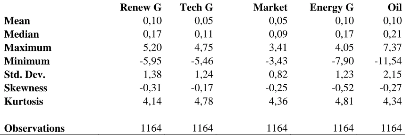
Tables 3 and 4 show the statistics summary of the daily compound returns, in

percentage, for all the variables. It can be observed from the table that indexes from the

same sector but from different geographic zones have relatively similar mean values and

with the same sign, exception being the Energy EU. A comparison for the global

indexes between the two periods shows the Market as the only variable with an increase

in mean from the first to the second period. Regarding volatility for global variables, it

has increased for Renewable G, Market and Energy G, opposing the trend shown by the

other variables.

Table 3 - Descriptive statistics of the daily compound returns, for the period 2002-2007.

Renew G Tech G Market Energy G Oil

Mean 0,10 0,05 0,05 0,10 0,10

Median 0,17 0,11 0,09 0,17 0,21

Maximum 5,20 4,75 3,41 4,05 7,37

Minimum -5,95 -5,46 -3,43 -7,90 -11,54

Std. Dev. 1,38 1,24 0,82 1,23 2,15

Skewness -0,31 -0,17 -0,25 -0,52 -0,27

Kurtosis 4,14 4,78 4,36 4,81 4,34

(25)

T ab le 4 De sc riptiv e sta ti sti

cs of the

(26)

4. Methodology

A vector autoregression (VAR) model was used in this work to study the

relationships amongst the variables: Renewable, Technology, Energy and Oil. This

model was chosen because a similar methodology to the study published by Sadorsky

and Henriques (2008) is being employed, where a VAR model was applied. A VAR

can be written in the following way:

In the equation above, y is an n vector of endogenous variables and is an n x n

matrix of the regression with the value of the parameters being estimated. The is the

error term of the equation which is assumed to be independent and following a normal

distribution with zero mean and a constant variance. In the equation shown above the

degrees of freedom are equal to n2p, where p is the number of lags. The number of lags

selection is a crucial part of the model seeing that if the number of lags is too high, it

will diminish the degrees of freedom which in turn lead to higher standard errors. On

the other hand, if the number of lags is too low, the VAR model may not capture all

relationships amongst the variables.

In order to estimate the VAR parameters, the variables need to be stationary.

Most economic variables are of order of integration equal to 1. Once the variables are

stationary, an Akaike Information Criteria (AIC) is conducted, using the respective

stationary variables in order to discover the appropriate number of lags to use in the

model. Subsequently, running a Johansen Test is necessary to understand if the

(27)

vector of error correction model (VECM), otherwise an Unrestricted VAR model can be

used.

Since the significance of the parameters estimated in the VAR are hard to

understand, it is advisable to perform a Granger causality test and then apply an Impulse

response function. The Granger causality test gives statistical information about which

variables have no impact in the value of a variable at the present. In the Impulse

response function test a shock of one standard deviation is given to one of the variables.

The output of the test is a graph which shows the response of each of the variables to

the shock, through a lag period. This enables to see if a shock has a negative/positive

impact on a variable, how it changes through time and how long it takes for the variable

to stabilize again. However, if there is no statistical evidence from the Granger

causality test from variable Y to X, then the importance of the Impulse response

(28)

5. Results and Discussion

5.1 Construction of the VAR models

In order to understand the order of integration of the data an Augmented

Dickey and Fuller test (ADF) and Kwiatkowski-Phillips-Schmidt-Shin test (KPSS) were

computed based on the logarithm of the variables. For the levels ADF test, the null

hypothesis (H0) is: the order of integration is equal to one (I(1)); while the alternative

hypothesis (H1) is: the order of integration is 0 (I(0)). For the levels KPSS test, the H0 is

I(0), while the H1 is I(1).

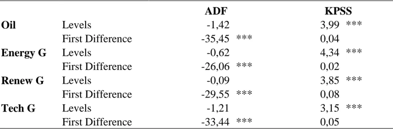
The results of the ADF and KPSS tests for both time periods are shown in tables

5 and 6. Doubts may arise concerning the order of integration of Renew G, Renew EU,

Energy US and Oil, for the second period. In the Appendix are the histograms of the

respective variables, figure A1 to A4, which are enlightening regarding this question.

The tests and the histograms demonstrate that the level of integration of all variables is

1. In order to build the VAR model, the variables need to be stationary and therefore the

VAR was constructed using the difference of the variables’ logarithm values - in other

words the returns were used.

Table 5 - Unit Roots are tested using (ADF) and (KPSS), for the period 2002-2007. ***, **, * denote a statistical significance of 1%, 5% and 10%, respectively.

ADF KPSS

Oil Levels -1,42 3,99 ***

First Difference -35,45 *** 0,04

Energy G Levels -0,62 4,34 ***

Renew G Levels -0,09 3,85 ***

Tech G Levels -1,21 3,15 ***

(29)

Table 6 - Unit Roots are tested using (ADF) and (KPSS), for the period 2009-2014. ***, **, * denote a statistical significance of 1%, 5% and 10%, respectively.

ADF KPSS

Renew G Levels -1,40 1,35 ***

First Difference -30,33 *** 0,56 **

Renew US Levels -1,57 2,25 ***

Renew EU Levels -1,65 1,56 ***

First Difference -31,92 *** 0,80 ***

Tech G Levels -0,46 3,91 ***

Tech US Levels -0,64 4,09 ***

Tech EU Levels -1,30 2,54 ***

Energy G Levels -1,43 2,96 ***

Energy US Levels -1,18 3,37 ***

Energy EU Levels -2,98 ** 0,40 **

Oil Levels -3,03 ** 1,45 ***

First Difference -34,33 *** 0,54 **

Once all variables were stationary it was conducted an Akaike Information

Criteria (AIC) in order to discover the appropriate number of lags of the VAR. Each test

contained the returns of Oil and the returns of the indexes on that region, in that specific

period. The AIC tests suggested that all the VAR models should be constructed with

one lag period. Regarding the Johansen Cointegration tests, which were done using the

same variables of the AIC, the results did not suggest the presence of cointegration for

the different models. Therefore Unrestricted VAR models with one lag period were

constructed for each region and each time period. Tables A1 till A4 in the Appendix

(30)

Tables A9 till A12 present the results of the Lagrange-multiplier test for serial

correlation. The results show no evidence of serial correlation.

5.2 Granger causality test and Impulse response function

In order to understand the relationship amongst the global variables a Granger

causality test was performed using an F-statistic test. For this test the null hypothesis is:

Variable X does not cause the variable Y.

Table 7 shows the Granger causality test results of the global variables for the

two periods, while table 8 shows the results of the Granger causality test separately for

the U.S. and Europe.

Table 7 - Granger causality test for the following variables: Oil, Tech G, Energy G and Renew G. The variable shown at the top of each set is the dependent variable. The test is conducted for the two periods: 2002-2007 and 2009-2014. ***, **, * denote a statistical significance of 1%, 5% and 10%, respectively.

Oil Tech G

2002-07 2009-14 2002-07 2009-14

Energy G 2,34 7,07 *** Oil 1,59 2,51

Renew G 0,10 0,08 Energy G 0,07 0,92

Tech G 0,02 0,32 Renew G 12,50 *** 0,62

Energy G Renew G

2002-07 2009-14 2002-07 2009-14

Oil 2,54 3,59 * Oil 1,85 0,39

Renew G 0,38 0,01 Energy G 15,79 *** 3,01 *

(31)

Table 8 - Granger causality test. The “X” after each variable may refer to US or EU, as shown in the second row. The variable shown at the top for each set is the dependent variable. The test is conducted for the period 2009-2014. ***, **, * denote a statistical significance of 1%, 5% and 10%.

Oil Tech X

US Europe US Europe

Energy X 4,03 ** 6,35 ** Oil 2,14 3,02 *

Renew X 1,84 3,55 * Energy X 0,07 2,61

Tech X 6,28 ** 5,13 ** Renew X 0,00 0,60

Energy X Renew X

US Europe US Europe

Oil 1,93 2,25

Oil 1,05 0,68

Renew X 0,49 2,46

Energy X 0,67 7,47 ***

Tech X 2,14 0,48

Tech X 1,34 1,90

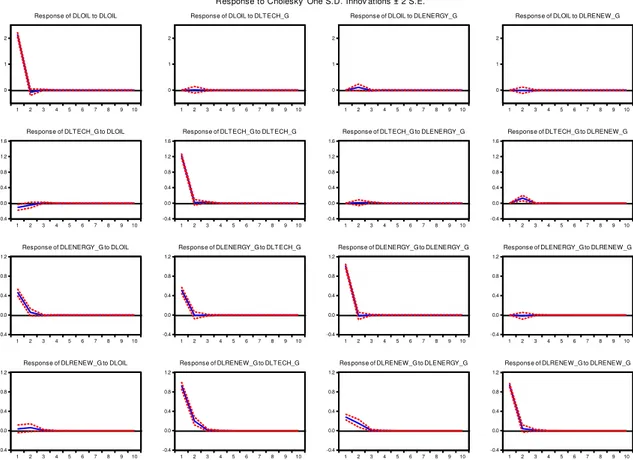
Figure 3 shows the Impulse response function using as variables: Oil, Tech G,

Energy G and Renew G, for the first period. The “DL”before the name of each variable

denotes the use of the difference of the logarithms as variables. Figure 4 shows the same

analysis as Figure 3 but for the period 2009-2014. The Impulse response functions using

American and European variables are shown in Figures 5 and 6, respectively. The

analysis of the Granger causality test and the Impulse response functions was made

together. Firstly, the results referent to the global data for both periods were analyzed.

Regarding Oil in the first period, there are statistical evidences that it does not

cause any of the variables and on the second period the null hypothesis is only rejected

for Energy G at a significance level of 10%. This result is in accordance with studies in

the literature, where it has been shown that only idiosyncratic demand shocks lead to

(32)

0 1 2

1 2 3 4 5 6 7 8 9 10

Response of DLOIL to DLOIL

0 1 2

1 2 3 4 5 6 7 8 9 10

Response of DLOIL to DLT ECH_G

0 1 2

1 2 3 4 5 6 7 8 9 10

Response of DLOIL to DLENERGY_G

0 1 2

1 2 3 4 5 6 7 8 9 10

Response of DLOIL to DLRENEW_G

-0.4 0.0 0.4 0.8 1.2 1.6

1 2 3 4 5 6 7 8 9 10

Response of DLT ECH_G to DLOIL

-0.4 0.0 0.4 0.8 1.2 1.6

1 2 3 4 5 6 7 8 9 10

Response of DLT ECH_G to DLT ECH_G

-0.4 0.0 0.4 0.8 1.2 1.6

1 2 3 4 5 6 7 8 9 10

Response of DLT ECH_G to DLENERGY_G

-0.4 0.0 0.4 0.8 1.2 1.6

1 2 3 4 5 6 7 8 9 10

Response of DLT ECH_G to DLRENEW_G

-0.4 0.0 0.4 0.8 1.2

1 2 3 4 5 6 7 8 9 10

Response of DLENERGY_G to DLOIL

-0.4 0.0 0.4 0.8 1.2

1 2 3 4 5 6 7 8 9 10

Response of DLENERGY_G to DLT ECH_G

-0.4 0.0 0.4 0.8 1.2

1 2 3 4 5 6 7 8 9 10

Response of DLENERGY_G to DLENERGY_G

-0.4 0.0 0.4 0.8 1.2

1 2 3 4 5 6 7 8 9 10

Response of DLENERGY_G to DLRENEW_G

-0.4 0.0 0.4 0.8 1.2

1 2 3 4 5 6 7 8 9 10

Response of DLRENEW_G to DLOIL

-0.4 0.0 0.4 0.8 1.2

1 2 3 4 5 6 7 8 9 10

Response of DLRENEW_G to DLT ECH_G

-0.4 0.0 0.4 0.8 1.2

1 2 3 4 5 6 7 8 9 10

Response of DLRENEW_G to DLENERGY_G

-0.4 0.0 0.4 0.8 1.2

1 2 3 4 5 6 7 8 9 10

Response of DLRENEW_G to DLRENEW_G Response to Cholesky One S.D. Innov ations ± 2 S.E.

Figure 3 - Impulse response function using as variables the difference of the logarithms of the Global variables, for the period 2002-2007.

for Energy G and at 5% for Tech G. Looking to the results of the Impulse response

function, figure 3, it can be concluded that a shock on Tech G has a higher impact than

one of Energy G, on Renew G. This result confirms the prediction that, during this

period, renewable energies were highly linked to technology. What is more, the fact that

at a significance level of 1%, for the same period, the null hypothesis of Renew G not

causing Tech G to be rejected suggests that renewable energy was perceived as a sub

sector of technology from 2002 to 2007. The expansion phases of the business cycle

that the world was facing on this period, coupled with high investment in clean energy

as mentioned in the literature due to high GDP’s, led to technology developments

in this area, which may explain the double causality. Nonetheless, the fact that the

(33)

-0.5 0.0 0.5 1.0 1.5 2.0

1 2 3 4 5 6 7 8 9 10

-0.5 0.0 0.5 1.0 1.5 2.0

1 2 3 4 5 6 7 8 9 10

Response of DLOIL to DLT ECH_G

-0.5 0.0 0.5 1.0 1.5 2.0

1 2 3 4 5 6 7 8 9 10

Response of DLOIL to DLENERGY_G

-0.5 0.0 0.5 1.0 1.5 2.0

1 2 3 4 5 6 7 8 9 10

Response of DLOIL to DLRENEW_G

-0.4 0.0 0.4 0.8 1.2

1 2 3 4 5 6 7 8 9 10

Response of DLT ECH_G to DLOIL

-0.4 0.0 0.4 0.8 1.2

1 2 3 4 5 6 7 8 9 10

Response of DLT ECH_G to DLT ECH_G

-0.4 0.0 0.4 0.8 1.2

1 2 3 4 5 6 7 8 9 10

Response of DLT ECH_G to DLENERGY_G

-0.4 0.0 0.4 0.8 1.2

1 2 3 4 5 6 7 8 9 10

Response of DLT ECH_G to DLRENEW_G

-0.2 0.0 0.2 0.4 0.6 0.8 1.0

1 2 3 4 5 6 7 8 9 10

Response of DLENERGY_G to DLOIL

-0.2 0.0 0.2 0.4 0.6 0.8 1.0

1 2 3 4 5 6 7 8 9 10

Response of DLENERGY_G to DLT ECH_G

-0.2 0.0 0.2 0.4 0.6 0.8 1.0

1 2 3 4 5 6 7 8 9 10

Response of DLENERGY_G to DLENERGY_G

-0.2 0.0 0.2 0.4 0.6 0.8 1.0

1 2 3 4 5 6 7 8 9 10

Response of DLENERGY_G to DLRENEW_G

-0.4 0.0 0.4 0.8 1.2

1 2 3 4 5 6 7 8 9 10

Response of DLRENEW_G to DLOIL

-0.4 0.0 0.4 0.8 1.2

1 2 3 4 5 6 7 8 9 10

Response of DLRENEW_G to DLT ECH_G

-0.4 0.0 0.4 0.8 1.2

1 2 3 4 5 6 7 8 9 10

Response of DLRENEW_G to DLENERGY_G

-0.4 0.0 0.4 0.8 1.2

1 2 3 4 5 6 7 8 9 10

Response of DLRENEW_G to DLRENEW_G Response to Cholesky One S.D. Innov ations ± 2 S.E.

Figure 4 - Impulse response function using as variables the difference of the logarithms of the Global variables, for the period 2009-2014.

energies are already efficient enough to compete with non-renewable energy and not so

dependent of technological breakthroughs anymore. Even though this might be true for

wind power, it is not yet a reality for solar energy. It would be therefore interesting, for

instance, to be able to split the renewable index into solar and wind indexes and

investigate if the theory would be confirmed. Moreover, this is the period after the

sub-prime crisis, where investments on the economies were low and consequently lower

technology developments were expected (Campello et al., 2010), which may have

led investors to see renewable energy as more dependent on governmental policies

and incentives. On the other hand, there is rejection of Energy G not Granger causing

(34)

0 1 2

1 2 3 4 5 6 7 8 9 10

0 1 2

1 2 3 4 5 6 7 8 9 10

Response of DLOIL to DLT ECH_US

0 1 2

1 2 3 4 5 6 7 8 9 10

Response of DLOIL to DLENERGY_US

0 1 2

1 2 3 4 5 6 7 8 9 10

Response of DLOIL to DLRENEW_US

-0.4 0.0 0.4 0.8 1.2 1.6

1 2 3 4 5 6 7 8 9 10

Response of DLT ECH_US to DLOIL

-0.4 0.0 0.4 0.8 1.2 1.6

1 2 3 4 5 6 7 8 9 10

Response of DLT ECH_US to DLT ECH_US

-0.4 0.0 0.4 0.8 1.2 1.6

1 2 3 4 5 6 7 8 9 10

Response of DLT ECH_US to DLENERGY_US

-0.4 0.0 0.4 0.8 1.2 1.6

1 2 3 4 5 6 7 8 9 10

Response of DLT ECH_US to DLRENEW_US

-0.4 0.0 0.4 0.8 1.2

1 2 3 4 5 6 7 8 9 10

Response of DLENERGY_US to DLOIL

-0.4 0.0 0.4 0.8 1.2

1 2 3 4 5 6 7 8 9 10

Response of DLENERGY_US to DLTECH_US

-0.4 0.0 0.4 0.8 1.2

1 2 3 4 5 6 7 8 9 10

Response of DLENERGY_US to DLENERGY_US

-0.4 0.0 0.4 0.8 1.2

1 2 3 4 5 6 7 8 9 10

Response of DLENERGY_US to DLRENEW_US

-0.5 0.0 0.5 1.0 1.5 2.0

1 2 3 4 5 6 7 8 9 10

Response of DLRENEW_US to DLOIL

-0.5 0.0 0.5 1.0 1.5 2.0

1 2 3 4 5 6 7 8 9 10

Response of DLRENEW_US to DLTECH_US

-0.5 0.0 0.5 1.0 1.5 2.0

1 2 3 4 5 6 7 8 9 10

Response of DLRENEW_US to DLENERGY_US

-0.5 0.0 0.5 1.0 1.5 2.0

1 2 3 4 5 6 7 8 9 10

Response of DLRENEW_US to DLRENEW_US Response to Cholesky One S.D. Innov ations ± 2 S.E.

Figure 5 - Impulse response function using as variables the difference of the logarithms of the U.S. variables, for the period 2009-2014.

There is also a small positive response of Renew G to the shock of Energy G in the

Impulse response function at a global level for both periods, figure 3 and 4, which

suggests that investors have seen renewable energy as a sub-sector of the energy

producing sector from 2002 onwards. The positive response to the shock was

unexpected since investors should had seen clean energy as competitor of

non-renewable energies. On the other hand, the increase in energy demand worldwide could

explain this result. Since the oil and gas index is recognized as a benchmark for the

energy producing sector, in times of energy demand increases, an increase in this index

would lead to increases in other related indexes, since they have the common goal of

being able to match the supply to cope with increases in demand. Still regarding the

(35)

0 1 2

1 2 3 4 5 6 7 8 9 10

0 1 2

1 2 3 4 5 6 7 8 9 10

Response of DLOIL to DLT ECH_EU

0 1 2

1 2 3 4 5 6 7 8 9 10

Response of DLOIL to DLENERGY_EU

0 1 2

1 2 3 4 5 6 7 8 9 10

Response of DLOIL to DLRENEW_EU

-0.4 0.0 0.4 0.8 1.2 1.6

1 2 3 4 5 6 7 8 9 10

Response of DLT ECH_EU to DLOIL

-0.4 0.0 0.4 0.8 1.2 1.6

1 2 3 4 5 6 7 8 9 10

Response of DLT ECH_EU to DLT ECH_EU

-0.4 0.0 0.4 0.8 1.2 1.6

1 2 3 4 5 6 7 8 9 10

Response of DLT ECH_EU to DLENERGY_EU

-0.4 0.0 0.4 0.8 1.2 1.6

1 2 3 4 5 6 7 8 9 10

Response of DLT ECH_EU to DLRENEW_EU

-0.4 0.0 0.4 0.8 1.2 1.6

1 2 3 4 5 6 7 8 9 10

Response of DLENERGY_EU to DLOIL

-0.4 0.0 0.4 0.8 1.2 1.6

1 2 3 4 5 6 7 8 9 10

Response of DLENERGY_EU to DLTECH_EU

-0.4 0.0 0.4 0.8 1.2 1.6

1 2 3 4 5 6 7 8 9 10

Response of DLENERGY_EU to DLENERGY_EU

-0.4 0.0 0.4 0.8 1.2 1.6

1 2 3 4 5 6 7 8 9 10

Response of DLENERGY_EU to DLRENEW_EU

-0.5 0.0 0.5 1.0 1.5

1 2 3 4 5 6 7 8 9 10

Response of DLRENEW_EU to DLOIL

-0.5 0.0 0.5 1.0 1.5

1 2 3 4 5 6 7 8 9 10

Response of DLRENEW_EU to DLTECH_EU

-0.5 0.0 0.5 1.0 1.5

1 2 3 4 5 6 7 8 9 10

Response of DLRENEW_EU to DLENERGY_EU

-0.5 0.0 0.5 1.0 1.5

1 2 3 4 5 6 7 8 9 10

Response of DLRENEW_EU to DLRENEW_EU Response to Cholesky One S.D. Innov ations ± 2 S.E.

Figure 6 - Impulse response function using as variables the difference of the logarithms of the European variables, for the period 2009-2014.

Energy G contradicts the predictions, in which a minor causality was to be expected

during this period since the major oil and gas companies were investing in this sector.

One explanation for the results might lie in investments from non-renewable energy

companies on clean energies being too low when compared to their companies sizes. A

lack of causality was also verified during the second time period analyzed but, in this

case, this was expected as studies have shown that the major oil and gas companies

have withdrawn their investment on clean energies during the course of this period

(Ferris and Gronewold, 2014).

An analysis of the results for the U.S. and Europe during 2009-2014 shows

similarities with the global indexes for the same time period, regarding renewable

(36)

with Energy US, where rejection of the null hypothesis is not verified. The Granger

causality test null hypothesis, being Renew EU the dependent variable, was rejected for

Energy EU at a significance level of 1%. This outcome goes in hand with the result

observed for the Global indexes for the same period. These results suggest a different

investors attitude depending on the region they live: while European investors see clean

energy as a energy production sector as global investors, American investors do not.

Additionally, since the null hypothesis was not rejected for Renew X to Tech X in both

cases, investors regardless of their location believe that clean energy is not dependent on

new technological developments. Because European policies are strict and investments

are high due to incentives, a lack of or low relationship between clean energies and

technology is somewhat expected. Incentives from the European Union may be leading

investors to see green energies as a sub-sector of the energy producing sector. In the

U.S. the level of investment in clean energies during this period is lower when

compared to Europe, the policies are still at a state level and not centralized yet. This

makes renewable energy more dependent on technological advances to reduce costs and

increase their efficiency so they can become a viable option. Therefore, rejection of the

null hypothesis for Tech US Granger causing Renew US was to be expected. However,

in a period of low investment and after a financial crisis, the technology sector was also

affected and this can explain the non-existence in causality revealed by the results

(Campello et al., 2010). Additionally, the investment in shale oil during this period

relegated investments on renewable energy to second place, which may also explain

(37)

6. Conclusion

This thesis analyses the relationships of clean energy with technology, oil and

gas companies, and oil prices. This study contributes to the existing literature by

updating data, including a non-renewable energy company’s index and by analyzing

two geographical regions.

The work here presented aimed to answer to the three following questions:

1) How does the global investor/market see renewable energy associated with the

technology sector, the oil and gas companies sector, as well as with oil prices

variations, from 2002-2007;

2) How has the investor’s perspective on clean energy changed over time, by

analyzing two distinct periods: 2002-2007 and 2009-2014;

3) How have different regions (Europe and U.S.) of the world seen these

relationships during the period from 2009 to 2014.

Regarding the first question, the results suggest the global investor in this period

perceived clean energy mainly as a sub-sector of the technology sector, as previously

stated in the literature. The results also suggest that from 2002 to 2007 investors begun

to perceive green energies as a weak sub-sector of the energy production sector. The

two energy sectors, renewable and non-renewable, were not seen as competitors but

rather as two sub-sectors with the same goal, where one is clearly bigger than the other

and therefore the causality has only one way. The results show that the oil price has no

(38)

With respect to the second question, the results suggest a perspective shift from

the investors after the global crisis as they believe renewable energy is no longer

dependent on the technology sector. With the crisis, companies have cut their budget

regarding investments and technology innovations, which might lead to the obtained

results. During this period, as in the first, investors kept the opinion that clean energy

was a sub-sector of the energy production sector.

Concerning the third question, in this period the U.S. reduced the importation of

oil by 30% when compared with the period before the Subprime crisis due to shale oil

extraction (Institute for Energy Research, 2015), while Europe continued to import the

same amount. This fact may explain the differences in policies and incentives with

regards to clean energy, which in turn influences the attitudes of investors. The

European Union and therefore Europe as a whole - since most of the countries of

Europe belong to the E.U. - kept its policies and incentives on clean energy and even set

future goals for them. These actions led European investors to see green energy as an

alternative to the existing methods of energy production. Contrarily, there was a lack of

policies and incentives in the U.S. in support of renewable energies, when comparing

with E.U.. Shale oil investment in the 2009-2014 period further led American investors

to move away from seeing renewable energy as an alternative energy production

(39)

7. Future Research

In order to improve on the knowledge of this field, the indexes should be

constructed under the same weight model, for instance all as market

capitalization-weighted indexes. Moreover, the development of the European and the American

indexes for the first period, 2002-2007, would give insights into how the investors

attitudes evolved in the two different regions. The addition of more geographical

regions would also enable a better understanding and comparison of investors attitudes

worldwide. Another interesting development would be the division of the renewable

energy index into the different types of existent clean energies and the addition of

nuclear and coal indexes to the model. These would allow a deeper understanding on

how the different types of green energy relate to technology and to the energy

production sector. Finally, the introduction of a dummy variable linked to government

policies and incentives on clean energy would allow to understand the vulnerability and

(40)

8. Bibliography

Apergis, N., Miller, S., 2009. “Do structural oil-market shocks affect stock prices?”.

Energy Economics 31, 569-575.

Awerbuch, S., Sauter, R., 2006. “Exploiting the oil-GDP effect to support renewable

deployment”. Energy Policy 34, 2805-2819.

Barsky, R., Kilian, L., 2004. “Oil and the macroeconomy since the 1970s”. National

Bureau of Economic Research 10855.

Bloomberg, 2014. Bloomberg Professional. Available at: Nova School of Business

and Economics (Accessed: June 2, 2015).

Bradsher, K., 2010. “China leading global race to make Clean Energy”. The New

York Times, 30th of January, 2010. www.nytimes.com (Accessed June of 2015)

Campello, M., Graham, J., Harvey, C., 2010. “The real effects of financial constraint:

Evidence from a financial crisis”. Journal of Financial Economics 97, 470-487.

Chang, T., Huang, C., Lee, M., 2009. “Threshold effect on economic growth rate of

the renewable energy development from a change in energy price: Evidence from

OECD countries”. Energy policy 37, 5796-5802.

Cox, P., Betts, R., Jones, C., Spall, S., Totterdell, I., 2000. “Acceleration of global

warming due to carbon-cycle feedbacks in a coupled climate model”. Nature 408, 184

-187.

European Commission, 2010. “A strategy for smart, sustainable and inclusive

(41)

Ferris, D., Gronewold, N., 2014. “Why the oil majors are backing away from

renewable energy”. Environment & Energy Publishing, LLC, 3rd of October, 2014.

http://www.eenews.net (Accessed June of 2015)

Friedman, L., 2010. “China leads major countries with $34.6 billions invested in clean

technology”. The New York Times, 25th of March, 2010. www.nytimes.com

(Accessed June of 2015)

Gan,L., Eskeland, G., Kolshus, H., 2007. “Green electricity market development:

Lessons from Europe and the US”. Energy Policy 35, 144-155.

Gormus, N., 2012. “Causality and Volatility Spillover Effects on Sub-Sector Energy

Portfolios”. PhD thesis, University of Texas at Arlington.

Gormus, N., Sarkar, S. 2014. “Alternative energy indexes and Oil”. Journal of

Accounting and Finance 14(4), 52-60.

Institute for Energy Research, 2015. “America’s shale boom reduced oil prices and

U.S. oil imports”. Institute for Energy Research, 19th of February, 2015.

http://instituteforenergyresearch.org (Accessed in September of 2015).

International Energy Agency, 2009. “World Energy Outlook, 2009”.

International Energy Agency, 2011. “World Energy Outlook, 2011”.

Kesicki, F., 2010. “The third oil price surge – What’s different this time?”. Energy

Policy 38, 1596-1606.

(42)

prices in the stock market?”. Japan and the World Economy 27, 1-9.

Martinot, E., 2010. “Renewable power for China: Past, present and future”. Front.

Energy Power Eng. China 4(3), 287-294.

Mohammadi, H., 2009. “Electricity prices and fuel costs: Long-run relations and

short-run dynamics”. Energy Economics 31(3), 503-509.

New Energy Finance, 2010. “Global Trends in Sustainable Energy Investment”.

Noguera, J., Pecchecnino, R., 2007. “OPEC and the international oil market: Can a

Cartel fuel the engine of economic development”. International Journal of Industrial

Organization 25, 187-199.

Pinkse, J., Buuse, D., 2012. “The development and the commercialization of solar PV

technology in the oil industry”. Energy Policy 40, 11-20.

Sadorsky, P., Henriques, I., 2008. “Oil prices and the stock prices of alternative energy

companies”. Energy Economics 30, 998-1010.

Snyder, B., Kasier, M., 2009. “A comparison of offshore wind power development in

Europe and the US: Patterns and drivers of development”. Applied Energy 86, 1845

-1856.

Szabó, S., Waldau, A., Szabó, M., Monforti-Ferrario, F., Szabó, L., Ossenbrink, H.,

2014. “European renewable government policies versus model predictions”. Energy

Strategy Reviews 2, 257-264.

United States Environmental Protection Agency. “State and Local Climate and Energy

(43)

United States Government Printing Office, Washington DC, 2006. “Economic Report

(44)

9. Appendix

-8 -6 -4 -2 0 2 4 6 8

I II III IV I II III IV I II III IV I II III IV I II III

2010 2011 2012 2013 2014

DLRENEW_G

Figure A2 -

-8 -4 0 4 8 12

2010 2011 2012 2013 2014

DLRENEW_EU

6.2 6.4 6.6 6.8 7.0 7.2 7.4 7.6 7.8 8.0

2010 2011 2012 2013 2014

LRENEW_EU

Figure A2 - Histograms of Renew EU for 2009-2014. The first graph is for the logarithm of the variable while the second is for the first difference of the variable logarithm.

6.6 6.8 7.0 7.2 7.4 7.6 7.8

2010 2011 2012 2013 2014

LRENEW_G

(45)

Table A1– Coefficients for the Unrestricted VAR model using Global variables with data from 2002-2007. For each coefficient: the first row is the coefficient value, the second row is the Standard Error and the third is the T-statistic.

DLOIL DLTECH_G DLENERGY_G DLRENEW_G

DLOIL(-1) -0.063268 -0.023137 0.029311 0.001135

(0.03288) (0.01886) (0.01884) (0.02081)

[-1.92394] [-1.22656] [ 1.55568] [ 0.05456]

-10 -8 -6 -4 -2 0 2 4 6

2010 2011 2012 2013 2014

DLENERGY_US -10.0 -7.5 -5.0 -2.5 0.0 2.5 5.0 7.5 10.0

2010 2011 2012 2013 2014

DLOIL 4.2 4.3 4.4 4.5 4.6 4.7 4.8

2010 2011 2012 2013 2014

LOIL

5.8 5.9 6.0 6.1 6.2 6.3

2010 2011 2012 2013 2014

LENERGY_EU

Figure A3 - Histograms of Energy EU for 2009-2014. The first graph is for the logarithm of the variable while the second is for the first difference of the variable logarithm.

Figure A4 - Histograms of Oil for 2009-2014. The first graph is for the logarithm of the variable while the second is for the first difference of the variable logarithm.

(46)

DLTECH_G(-1) -0.027737 -0.078747 0.015673 0.071134

(0.07042) (0.04039) (0.04035) (0.04455)

[-0.39389] [-1.94956] [ 0.38847] [ 1.59662]

DLENERGY_G(-1) 0.103808 -0.026561 -0.013220 0.137541

(0.06423) (0.03684) (0.03680) (0.04063)

[ 1.61631] [-0.72099] [-0.35926] [ 3.38482]

DLRENEW_G(-1) -0.010277 0.139135 -0.018602 0.043093

(0.06433) (0.03690) (0.03686) (0.04070)

[-0.15976] [ 3.77070] [-0.50473] [ 1.05881]

C 0.093915 0.042085 0.102218 0.075594

(0.06337) (0.03635) (0.03631) (0.04010)

[ 1.48193] [ 1.15773] [ 2.81519] [ 1.88534]

Table A2 – Coefficients for the Unrestricted VAR model using Global variables with data from 2009-2014. For each coefficient: the first row is the coefficient value, the second row is the Standard Error and the third is the T-statistic.

DLOIL DLTECH_G DLENERGY_G DLRENEW_G

DLOIL(-1) -0.071867 0.032093 0.050701 -0.009381

(0.03666) (0.02511) (0.02980) (0.03273)

[-1.96038] [ 1.27802] [ 1.70144] [-0.28664]

DLTECH_G(-1) -0.150222 -0.068415 -0.156637 -0.138700

(0.08991) (0.06158) (0.07308) (0.08026)

[-1.67088] [-1.11093] [-2.14340] [-1.72816]

DLENERGY_G(-1) 0.288941 0.009367 0.009622 0.157106

(0.07610) (0.05212) (0.06185) (0.06793)

[ 3.79710] [ 0.17970] [ 0.15557] [ 2.31277]

DLRENEW_G(-1) -0.068369 0.019332 0.044670 0.096636

(0.05839) (0.03999) (0.04746) (0.05212)

[-1.17100] [ 0.48339] [ 0.94126] [ 1.85411]

C 0.021902 0.051282 0.042363 -0.010103

(0.04832) (0.03310) (0.03927) (0.04313)

(47)

Table A3 - Coefficients for the Unrestricted VAR model using US variables with data from 2009-2014. For each coefficient: the first row is the coefficient value, the second row is the Standard Error and the third is the T-statistic.

DLOIL DLTECH_US DLENERGY_US DLRENEW_US

DLOIL(-1) -0.037751 0.023187 0.026091 0.027503

(0.02928) (0.01585) (0.01843) (0.02604)

[-1.28941] [ 1.46301] [ 1.41599] [ 1.05627]

DLTECH_US(-1) -0.218818 -0.037128 -0.093948 -0.088130

(0.11255) (0.06093) (0.07083) (0.10009)

[-1.94422] [-0.60940] [-1.32633] [-0.88048]

DLENERGY_US(-1) -0.020706 0.013193 0.028902 -0.018124

(0.08397) (0.04546) (0.05285) (0.07468)

[-0.24658] [ 0.29024] [ 0.54689] [-0.24270]

DLRENEW_US(-1) 0.075857 -0.003327 0.005630 0.099986

(0.06009) (0.03253) (0.03782) (0.05344)

[ 1.26245] [-0.10229] [ 0.14887] [ 1.87105]

C 0.118650 0.068616 0.047850 -0.030512

(0.06358) (0.03442) (0.04002) (0.05655)

[ 1.86610] [ 1.99353] [ 1.19578] [-0.53960]

Table A4 - Coefficients for the Unrestricted VAR model using EU variables with data from 2009-2014. For each coefficient: the first row is the coefficient value, the second row is the Standard Error and the third is the T-statistic.

DLOIL DLTECH_EU DLENERGY_EU DLRENEW_EU

DLOIL(-1) -0.039775 0.035040 0.028052 0.018788

(0.02930) (0.02074) (0.01937) (0.02445)

[-1.35747] [ 1.68955] [ 1.44823] [ 0.76855]

DLTECH_EU(-1) -0.027461 -0.047585 -0.004244 -0.021794

(0.07855) (0.05559) (0.05192) (0.06553)

[-0.34962] [-0.85593] [-0.08174] [-0.33258]

DLENERGY_EU(-1) -0.090440 0.108004 0.096484 0.158726

(0.08030) (0.05684) (0.05309) (0.06700)

[-1.12622] [ 1.90018] [ 1.81752] [ 2.36911]

(48)

[ 0.05876] [-1.23701] [-1.35522] [-0.24434]

C 0.101139 0.030843 -0.003953 -0.039343

(0.06318) (0.04472) (0.04176) (0.05271)

[ 1.60088] [ 0.68976] [-0.09466] [-0.74642]

Table A5 - Fit of Unrestricted VAR Model with 1 lag, using Global variables with data from 2002-2007.

Determinant resid. covariance (dof adj.) 6.454902

Determinant resid covariance 6.344611

Log likelihood -7675.285

Akaike information criterion 13.23351

Schwarz criterion 13.32050

Table A6 - Fit of Unrestricted VAR Model with 1 lag, using Global variables with data from 2009-2014.

Table A7 - Fit of Unrestricted VAR Model with 1 lag, using American variables with data from 2009-2014

Table A8 - Fit of Unrestricted VAR Model with 1 lag, using European variables with data from 2009-2014.

(49)

Table A9 - Lagrange-multiplier test for the VAR model using Global variables, from 2002-2007.

Lags LM-Stat Prob

1 24.54366 0.0783

Table A10 - Lagrange-multiplier test for the VAR model using Global variables, from 2009-2014.

Lags LM-Stat Prob

1 14.79631 0.5396

Table A11 - Lagrange-multiplier test for the VAR model using American variables, from 2009-2014.

Lags LM-Stat Prob

1 8.961997 0.9150

Table A12 - Lagrange-multiplier test for the VAR model using European variables, from 2009-2014.

Lags LM-Stat Prob

The relationships of alternative energies with the technology sector and non-renewable energies

Escola de Economia de Empresas de São Paulo

Ricardo Miguel Silva Barão

The relationships of Alternative Energies

with the Technology Sector

and non-Renewable Energies

Ricardo Miguel Silva Barão

The relationships of Alternative Energies

with the Technology Sector

and non-Renewable Energies

The relationships of Alternative Energies

with the Technology Sector

and non-Renewable Energies

Acknowledgements

Resumo

Abstract

Table of Contents

1.

Introduction

2.

Literature Review

3.

Data

4.

Methodology

5.

Results and Discussion

6.

Conclusion

7.

Future Research

8.

Bibliography

9.

Appendix