A benchmark-based method to derive metric thresholds

(1)

A BENCHMARK-BASED METHOD TO DERIVE

(2)

(3)

GUSTAVO ANDRADE DO VALE

A BENCHMARK-BASED METHOD TO DERIVE

METRIC THRESHOLDS

Dissertação apresentada ao Programa de Pós-Graduação em Ciência da Computação do Instituto de Ciências Exatas da Univer-sidade Federal de Minas Gerais – Departa-mento de Ciência da Computação

como requisito parcial para a obtenção do grau de Mestre em Ciência da Computação.

Orientador: Eduardo Magno Lages Figueiredo

Belo Horizonte

(4)

(5)

GUSTAVO ANDRADE DO VALE

A BENCHMARK-BASED METHOD TO DERIVE

METRIC THRESHOLDS

Dissertation presented to the Graduate Program in Ciência da Computação of the Universidade Federal de Minas Gerais – De-partamento de Ciência da Computação in partial fulfillment of the requirements for the degree of Master in Ciência da Com-putação.

Advisor: Eduardo Magno Lages Figueiredo

Belo Horizonte

(6)

c

Vale, Gustavo Andrade do

V149b A Benchmark-based Method to Derive Metric Thresholds / Gustavo Andrade do Vale. — Belo Horizonte, 2016

xx, 76 f. : il. ; 29cm

Dissertação (mestrado) — Universidade Federal de Minas Gerais – Departamento de Ciência da

Computação

Orientador: Eduardo Magno Lages Figueiredo

1. Computação – Teses. 2. Engenharia de software – Teses. 3. Software – Reutilização – Teses. I.

Orientador. II. Título.

(7)

(8)

(9)

Acknowledgments

This work would not have been possible without the support of many people.

I thank God to provide me the discipline and persistence to reach a Master degree.

I thank my dear wife Fernanda, who has had patience in difficult moments and has always been by my side.

I thank my whole family — especially my father Fernando, my mother Marcia, my sister Leticia, my father-in-law Tom, my mother-in-law Regina and my sister-in-law Paula — for having always supported me.

I thank my advisor E. Figueiredo for his attention, motivation, patience, dedication, and immense knowledge. I certainly could not complete my Master study without him.

I thank L. Veado, E. Fernandes, R. Abilio, H. Costa, D. Albuquerque for the valuable collaboration in the case studies.

I thank the members of the LabSoft research group for the friendship and technical collaboration.

I would like to express my gratitude to the members of my dissertation defense — A. Garcia (PUC-Rio), K. A. M. Ferreira (CEFETMG) and M. T. Valente (UFMG).

I thank Capes and PPGCC-UFMG for the financial support.

(10)

(11)

Resumo

Com o crescimento em tamanho e complexidade dos sistemas de software, melhores suportes são requeridos para medir e controlar a qualidade de software. Métricas de software são um caminho prático para avaliar diferentes atributos e características de qualidade, como tamanho, complexidade, manutenibilidade e usabilidade. Apesar disso, apenas os valores de métricas não são suficientes. A medição efetiva de sistemas de software é diretamente dependente da definição de valores limiares apropriados. Valores limiares permitem caracterizar objetivamente ou classificar cada componente de acordo com uma métrica de software. A definição de valores limiares apropriados precisa ser calculada para cada métrica. Com o objetivo de investigar este tópico, uma revisão sistemática da literatura de métodos para calcular valores limiares foi realizada. Nesta revisão, foi analisada a evolução de tais métodos e percebeu-se que pesquisadores e profissionais da indústria não possuem um consenso sobre as caracterís-ticas de tais métodos. De fato, muitos métodos têm sido propostos e utilizados nos últimos anos. Após a revisão da literatura, foi realizado um detalhado estudo compar-ativo de três métodos recentemente propostos para calcular valores limiares (métodos de Alves, Ferreira e Oliveira). Nessa comparação são destacadas as principais carac-terísticas de cada método e, como lições aprendidas, baseado no conhecimento teórico e prático adquirido, são apresentados oitos pontos desejáveis para este tipo de método. Almejando cobrir todos os pontos desejáveis e capturar o melhor de cada método, um método é proposto para calcular valores limiares para métricas, chamado Vale’s method. Este método foi devidamente descrito, cada passo do método foi justificado e uma ferramenta para apoiar o método proposto e os métodos comparados foi de-senvolvida. No total derivaram-se valores limiares para 8 métricas de software. Para avaliar o método proposto, (i) analisaram-se os valores limiares individualmente e uti-lizando uma estratégia baseada em métricas, (ii) analisaram-se os resultados utiuti-lizando duas bases de dados com métricas de diversos sistemas de dois diferentes tipos, e (iii) forneceu-se uma visão geral do método proposto comparado com outros métodos pre-sentes na literatura. Em resumo, todos os métodos estudados parecem ser justos para

(12)

calcular valores limiares para métricas de software, no entanto, o método proposto se saiu melhor nas avaliações.

Palavras-chave: Qualidade de Software, Métricas de Software, Valores Limiares, Métodos para Calculo de Valores Limiares.

(13)

Abstract

With softwaintensive systems growing in size and complexity, better support is re-quired for measuring and controlling the software quality. Software metrics are the practical means for assessing different quality attributes and characteristics, such as size, complexity, maintainability, and usability. In spite of that, only the values of metrics are not enough. The effective measurement of software systems is directly de-pendent on the definition of appropriate thresholds. Thresholds allow to objectively characterize or to classify each component according to one of the software metrics. The definition of appropriate thresholds needs to be tailored to each metric. Aiming to investigate this topic, we first performed a literature review of methods to derive thresholds. In this review, we analyzed the evolution of such methods and realized that researchers and practitioners do not have a consensus about the characteristics of these methods. In fact, many methods have been proposed and have been used in the lasts years. After the literature review, we present a detailed comparison of three re-cently proposed methods to derive metric thresholds (Alves’s, Ferreira’s, and Oliveira’s methods). This comparison highlights the main characteristics of each method and, as lessons learned, we present eight desirable points for this kind of method based on our theoretical and practical knowledge. Trying to fit all desirable points and getting the best of each method, we propose our own method to derive metric thresholds, named Vale’s method. We explain our method, justifying each of its steps, and develop a tool to support the method, called TDTool. In the total we provide thresholds for 8 metrics. To evaluate Vale’s method, we (i) analyzed the derived thresholds individ-ually and using a metric-based detection strategy, (ii) analyzed the results using two different types of benchmarks, and (iii) provided an overview of the method compared to other methods in the literature. In summary, all the compared methods seem to be fair to derive metric thresholds, but our method fared better in the evaluations.

Keywords: Software Quality, Metric, Thresholds, Method to Derive Thresholds.

(14)

(15)

List of Figures

1.1 Lazy Class Detection Strategy (Adapted from [Munro, 2005]) . . . 2

2.1 Features, Constants, and Refinements relationship . . . 9

2.2 Example of code (adapted from [Kastner and Apel, 2008]) . . . 9

2.3 Examples of Computing Metrics . . . 10

3.1 Metric Thresholds Side by Side . . . 28

4.1 Summary of the Method Steps . . . 36

4.2 Probably Density Function . . . 38

4.3 Probably Density Function [Ferreira et al., 2012] . . . 39

4.4 TDTool Overview . . . 40

4.5 TDTool Stages . . . 41

4.6 Example of Input File for TDTool . . . 41

4.7 Metrics Selection . . . 42

4.8 Final Results . . . 43

4.9 Code Smells Detection Strategy . . . 45

5.1 Derived Thresholds for 7 Metrics Using Benchmark 4 . . . 56

5.2 Derived Thresholds from SPL and Java Benchmark Side-by-Side . . . 58

(16)

(17)

List of Tables

3.1 Software Product Lines Benchmarks . . . 23

3.2 Correlation of Metrics with LOC . . . 24

3.3 Weibull Values for Each Metric per Benchmark . . . 25

3.4 Threshold Values from Alves’s Method . . . 26

3.5 Threshold Values from Ferreira’s Method . . . 26

3.6 Threshold Values from Oliveira’s Method . . . 27

3.7 Comparative Evaluation of the Method for Calculating Thresholds . . . 30

4.1 Code Smell Oracle for MobileMedia . . . 46

4.2 Threshold Values from the Proposed Method . . . 47

4.3 Identification of Code Smells Based on Thresholds Derived From the Pro-posed Method . . . 48

5.1 Identification of God Classes based on Derived Thresholds of Each Method 52 5.2 Threshold Value from Four Studied Methods . . . 55

6.1 Evolution in the Threshold Calculation Literature . . . 63

A.1 List of Papers of Our Literature Review . . . 73

A.2 List of Papers of Our Literature Review (Cont.1) . . . 74

(18)

(19)

Chapter 1 Introduction

With softwaintensive systems growing in size and complexity, better support is re-quired for measuring and controlling the software quality [Gamma et al., 1995]. Soft-ware metrics are the practical means for assessing different quality attributes, such as maintainability and usability [Chidamber and Kemerer, 1994; Lorenz and Kidd, 1994]. Certain metric values can help to reveal specific components (or modules) of a software system that should be closely monitored [Dumke and Winkler, 1997]. For instance, such measures can be used to indicate whether a critical anomaly (or smell) is affecting a component structure [Riel, 1996].

Although software metrics are the pragmatic means for assessing different quality attributes, only the values of metrics are not enough. The effective measurement of software systems is directly dependent on the definition of appropriate thresholds. Thresholds allow to objectively characterize or to classify each entity (e.g. module, class, method) according to one of the quality metrics. The definition of appropriate thresholds needs to be tailored to each metric.

1.1 Motivation, Problem Description, and Goal

Thresholds have a high influence in the software quality measurement. Additionally, as software systems have been increasing in size and complexity in the past few years, thresholds must be calculated in a specific context, avoiding generic or global thresh-olds. However, it is necessary methods easy to use, simple, and fair to derive threshthresh-olds. Given the necessity we want to know:

• What are the methods to derive metric thresholds?

• What are the main characteristics of methods to derive thresholds?

(22)

2 Chapter 1. Introduction

• What is desirable for methods to derive thresholds?

• Do a method better than another? Based on its characteristics?

Given these four questions, we start a literature review to answer them. We could see that in the past few years, thresholds were calculated based on software engineers’ experience or by using a single system as reference [Chindamber and Kemerer, 1994; Coleman et al., 1995; Erni and Lewerentz, 1996; French, 1999; McCabe, 1976; Nejmeh, 1988; Spinellis, 2008; Vasa et al., 2009]. Recently, it has been changing and thresholds have been calculated considering three key points [Alves et al., 2010; Ferreira et al., 2012; Oliveira et al., 2014]: (i) well-defined methods, (ii) methods that consider the skewed distribution of software measurements, and, (iii) methods which use data from benchmarks.

Although we have found many studies about thresholds calculation, the recent improvements in methods to derive thresholds indicate an open field to explore this re-search topic and we did not find any comparative study of methods to derive thresholds. Additionally, methods previously proposed in literature do not address important as-pects when metric-based strategies are used, such as the lower bound thresholds. Lower bound thresholds can be useful for identifying lazy class, for example. Lazy class is a bad smell defined as a class that knows or does too little in the software system [Fowler et al., 1999].

Figure 1.1 presents a detection strategy to identify lazy class instances [Munro, 2005] which combine three metrics (Lines of Code (LOC) [Fenton and Pfleeger, 1998], Weight Method per Class (WMC) [Chidamber and Kemerer, 1994], and, Coupling between Objects (CBO) [Chidamber and Kemerer, 1994]) with logical operators (AND and OR). Note that for each metric a specific threshold is required. According to this detection strategy, for a class be a lazy class instance, it should have LOC and WMC smaller than threshold of these metrics; or CBO smaller than threshold of this metric.

(23)

1.2. Methodological Procedures and Contributions ₃

Additionally to lower bound thresholds, as we are going to see in this disserta-tion, we compared three methods recently proposed, which address the three key points previously mentioned. With this comparison, we described eight desirable points ex-tracted based on our theoretical and practical experience. Following these desirable points, the methods should: (i) be well-defined and deterministic; (ii) derive thresh-olds in a step-wise format; (iii) be weakly dependent on the number of systems; (iv) be strongly dependent on the number of entities; (v) not correlate metrics; (vi) calcu-late upper and lower thresholds; (vii) provide representative thresholds independent of metric distribution and (viii) provide tool support. These desirable points were used as motivation to propose our own method to derived metric thresholds, called Vale’s method.

Our method is organized in the five following steps: (i) metric extraction, (ii) weight ratio calculation, (iii) sort in ascending order, (iv) entity aggregation, (v) thresh-olds derivation. In summary, we need to extract the metric values of the target entities (which composes the benchmark) to give the same weight for each entity. The sum of all entities represents 100%. After, we should organize the entities by the value of the selected metric. Then, we should sum up the entities with same value. Finally, we should to derive the thresholds for each one of the labels of the method (verylow,

low,moderate, high, and veryhigh). It is important to highlight that for each metric these steps should be followed. Additionally, we provide a tool to support our method and, the proposed method was evaluated in different ways, it is better explained on the next section.

The main goal of this dissertation is to propose a method to derive metric thresh-olds addressing the eight desirable points that previous proposed methods do not ad-dress, but these desirable points are important to derive appropriate thresholds.

1.2 Methodological Procedures and Contributions

(24)

4 Chapter 1. Introduction

points previous mentioned: Alves’s [Alves et al., 2010], Ferreira’s [Ferreira et al., 2012] and Oliveira’s [Oliveira et al., 2014] methods.

Then, we provide a comparative study with the highlighted methods using 3 benchmarks composed by software product lines (SPLs). An SPL is a configurable set of systems that shares a common, managed set of features in a particular market segment [SEI, 2016]. Features can be defined as modules of an application with consistent, well-defined, independent, and combinable functions [Apel et al., 2009]. We decided to build SPL benchmarks because of SPLs tend to be systems more modularized than single systems and they are been increasingly adopted in software industry to support coarse-grained reuse of software assets [Dumke and Winkler, 1997]. To build these benchmarks, we looked for papers and repositories about SPLs. Chapter 3 gives more details about the SPL benchmarks.

With the comparative study, we pointed out some desirable points based on theoretical and practical knowledge applying the three methods. With these desirable points, we find the opportunity to propose a method (third task). For example, Alves’s, Ferreira’s, and Oliveira’s methods do not present lower bound thresholds. Additionally, we can find aspects addressed by one method, but not addressed by other methods, such as, to present thresholds in a step-wise format.

After the comparative study, we propose our own method, called Vale’s method. The proposed method is descripted and we present a complete example of use. Addi-tionally, in the third task, we provide a tool, called TDTool, to support the proposed method and other three methods (Alves’s, Ferreira’s, and Oliveira’s methods).

Finally, on the forth task, we evaluate the proposed method using different con-texts, benchmarks, and in different ways, such as the effectiveness in detecting bad smells and analyzing the values individually. In the total, we derive thresholds for eight different metrics. In the case of benchmarks, we use three benchmarks composed by SPLs and one composed by single systems developed using Java. Differently to the SPL benchmarks, the Java benchmark was previously proposed and used in another studies.

1.3 Dissertation Outline

This master dissertation is organized in 6 chapters, as follows.

(25)

1.3. Dissertation Outline ₅

Chapter 3 presents a comparative study of methods to derive thresholds high-lighting desirable points pointed out in this comparison.

Chapter 4 describes the proposed method, called Vale’s method, based on the desirable points, presented in previous chapter, and a tool to support the proposed method and other three methods, called TDTool.

Chapter 5 evaluates the proposed method considering different aspects, such as using different benchmarks and benchmarks from different contexts.

(26)

(27)

Chapter 2 Background

This chapter presents important concepts to understand this dissertation. These main concepts involve three main topics: software product lines (SPLs), metrics, and meth-ods to derive metric thresholds. Section 2.1 starts with some important concepts about SPLs and feature-oriented programming because we build a benchmark composed by SPLs on the next chapter and, we use a metric specific to SPLs. Then, Section 2.2 intro-duces the concept of metrics and the metrics used in this dissertation. After, the next sections are related to the literature review and concepts about metrics to derive thresh-olds. Therefore, Section 2.3 presents our protocol to get methods to derive threshthresh-olds. Section 2.4 presents the results of our literature review and the different types of these methods. Section 2.5 discusses the importance of three fundamental points of methods to derive thresholds. We called these points of three key points. These key points are: (i) methods well-defined, (ii) methods that consider the skewed distribution of software measurements, and, (iii) methods that use benchmarks as database to derive thresholds. Section 2.6 describes three methods which address these three key points. These methods are explored in this dissertation and, because of that we present them in a separate section. Finally, Section 2.7 summarizes Chapter 2.

2.1 Software Product Lines

Software Product Line (SPL) is a set of software systems that share a common, man-aged set of features satisfying the specific needs of a particular market segment [Pohl and Metzer, 2006]. The systematic and large scale reuse adopted in SPLs aim to re-duce time-to-market and improve software quality [Pohl et al., 2005]. The software products derived from an SPL share common features and differ themselves by their specific features [Pohl et al., 2005]. A feature represents an increment in functionality

(28)

8 Chapter 2. Background

or a system property relevant to some stakeholders [Kastner et al., 2007]. And, features can be defined as modules with consistent, well-defined, independent, and combinable functions [Apel et al., 2009]. The possible combinations of features to build a product are called SPL variability [Weiss and Lai, 1999] and it can be represented in a feature model [Kang et al., 1990]. Feature model is a formalism to capture and to represent the commonalities and variabilities among the products in an SPL [Asikainen et al., 2006].

In order to develop an SPL, we can use different approaches, such as, annotative [Liebig et al., 2010] and compositional [Apel and Kastner, 2009]. For these approaches, there are several techniques, for example, preprocessors [Liebig et al., 2010], virtual separation of concerns [Kastner et al., 2008], aspect-oriented programming [Kiczales et al., 1997], delta-oriented programming [Schaefer et al., 2011], and feature-oriented programming [Batory et al., 2003]. These approaches and techniques aim to support configuration management at source code level and improve the software quality.

Feature-oriented programming (FOP) is a compositional technique to develop SPLs. There are many feature-oriented languages and tools aiming at feature mod-ularity, e.g., AHEAD/Jak [Batory et al., 2004], FeatureC++ [Apel et al., 2005], and FeatureHouse [Apel et al., 2009]. In this section, we use AHEAD as a representative for FOP compositional approaches. AHEAD is based on the concept of step-wise re-finements. Step-wise refinement is a paradigm to develop a complex program from a simple program by incrementally adding details [Batory et al., 2003]. The program increments and original fragments are called refinements and constants, respectively [Batory et al., 2003]. Classes (constants) implement basic functions of a system and extensions in these functions constitute the class refinements. The AHEAD Tool Suite (ATS) was developed to support FOP in AHEAD and it has tools for realization and composition of features [Batory, 2004]. ATS relies on the Jakarta (Jak) programming language (superset of Java) [Batory, 2004]. Constants and refinements are defined in Jak files, but constants are pure Java-code and refinements are identified by the keyword ref ines.

(29)

2.2. Software Metrics ₉

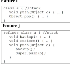
Figure 2.1: Features, Constants, and Refinements relationship

Figure 2.2 depicts a code example in AHEAD. The ai class implements a stack with two methods: push and pop. The refines keyword in aj class indicates that aj refines ai. In this example, the aj class adds new methods (backup() and restore()) and extends the behavior of thepush()method (in the ai class) by adding the calling of

backup() method. The calling of push() method in the refinement chain is performed using the Super keyword. We use ATS to compose base code and different feature modules. Different products are generated according to inclusion of features in the composition process [Kastner and Apel, 2008].

Figure 2.2: Example of code (adapted from [Kastner and Apel, 2008])

2.2 Software Metrics

(30)

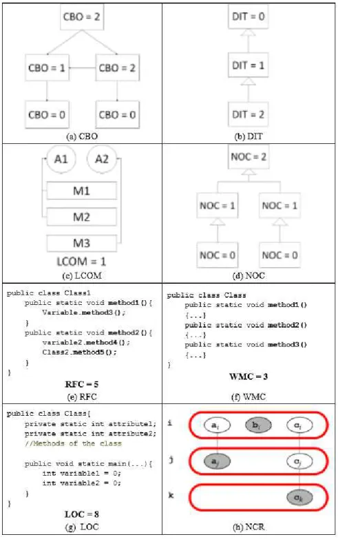
as size, coupling, cohesion, and complexity using metrics. In this work, we use the eight following metrics: Coupling between Objects, Depth of Inheritance Tree,Lack of Cohe-sion in Methods, Number of Children, Response for a Class, Weight Method per Class, Lines of Code, and Number of Constant Refinements. Figure 2.3 provides examples of applying each of the eight metrics:

(31)

2.2. Software Metrics ₁₁

• Coupling between Objects (CBO) (Chidamber and Kemerer 1994) counts the number of classes called by a given class. CBO measures the degree of coupling among classes. Figure 1.3(a) illustrates an example of how CBO is calculated. In that example, each box represents classes and each arrow represents a relation between two classes.

• Depth of Inheritance Tree (DIT) (Chidamber and Kemerer 1994) counts the number of levels that a subclass inherits methods and attributes from a superclass in the inheritance tree of the system. This is another metric to estimate the class complexity/coupling. Figure 1.3(b) presents an example of DIT computation. As can be seen in Figure 1.3(b), a class has DIT = 0, the subclass of this class has DIT = 1 and, successively.

• Lack of Cohesion in Methods (LCOM) (Chidamber and Kemerer 1994) counts the number of method pairs whose access non-common attributes, minus the count of method pairs whose access common attributes. The larger the number of similar methods, the more cohesive the class. For instance, in Figure 1.3(c), M1, M2, and M3 are methods. The pairs M1-M3 and M2-M3 do not access the attribute A1. On the other hand, the pair M1-M2 accesses the attribute A1. Therefore, LCOM = 1.

• Number of Children (NOC) (Chidamber and Kemerer 1994) counts the number of direct subclasses of a given class. This metrics indicates code reuse. Figure 1.3(d) presents an example of computed NOC. For instance, the class higher up in inheritance tree has two derived classes at the immediately below level, that extends the parent class. Therefore, this class has NOC = 2. In turn, the classes at the lowest levels have no derived classes that extend them. Therefore, NOC = 0.

• Response for a Class (RFC) (Chidamber and Kemerer 1994) is a set of methods that can potentially be executed in response to a message received by an object of that class. This metric supports the assessment of class complexity. Figure 1.3(e) presents an example of RFC computing. In this figure, the sample class implements two methods, and it calls three methods from other classes. These five methods may be called depending on the use of instantiate objects of the illustrative class. Therefore, RFC = 5.

(32)

counting the number of methods in a class. This metric can be used to estimate the complexity of a class. Figure 1.3(f) illustrates how WMC is computed when considering the number of method as a weight. For each method present in a class, we increment the value of WMC. Therefore, in case of Figure 1.3(f) in which there are three methods, WMC = 3.

• Lines of Code (LOC) (Lorenz and Kidd 1994) counts the number of uncommented lines of code per class. The value of this metric indicates the size of a class. Figure 1.3(g) presents an illustrative example of computed LOC. LOC counts code lines, but LOC does not count neither comment lines nor blank lines. In Figure 1.3(g), LOC is equals to 8.

• Number of Constant Refinements (NCR) (Abilio et al. 2015) counts the number of refinements that a constant has. Its value indicates how complex the relation-ship between a constant and its features is. Constants and refinements are files that can often be found in Feature-Oriented Programming (FOP) (Batory, 2004). That is, refinements can change the behavior of a constant if certain feature is included in a product (see Section 2.1). Figure 1.3(h) presents an example of computed NCR. In Figure 1.3(h), we have the features i, j, and k; classes a, b, and, c; ai, bi, ci are constants of feature i; aj, cj, ck are refinements of feature j and k. Therefore, constants ai, bi, and ci have NCR equal to 1, 0, and, 3, respectively.

We chose LOC, CBO, WMC, and, NCR because of the metric-based detection strategies that we are going to use in this dissertation. Moreover, we included other metrics to cover all the six well-known object-oriented software metrics proposed by Chidamber and Kemerer (1994): CBO, DIT, LCOM, NOC, RFC, and WMC. For all eight metrics described, classes with higher values are more likely to be worse in the software systems quality.

2.3 Literature Review Protocol

(33)

2.3. Literature Review Protocol ₁₃

that propose metrics and thresholds [McCabe 1976; Nejmeh, 1988; Chidamber and Kemerer, 1994; Erni et al., 1996; Lanza and Marinescu, 2006; Ferreira et al., 2012]. Generally, studies that propose thresholds present a method or strategy to derive such thresholds.

This section summarizes how we got the papers related to methods to derive thresholds. First, we started an ad-hoc literature review held in four different electronic databases: IEEExplore 1

, Science Direct2

, ACM Digital Library3

, and El Compendex

4

. With this ad-hoc literature review, we found a systematic literature review (SLR) [Lima, 2014] with a similar, but different purpose of ours. An SLR is a well-defined method to identify, evaluate, and interpret all relevant studies regarding a particular research question, topic area, and phenomenon of interest [Kitchenham and Charters, 2007]. This existing SLR of Lima [2014] aims to group metric thresholds reported in the literature, but it does not focus on methods to derive thresholds.

The previous SLR was used as a starting point for our work. It selected 19 pa-pers to get and report information. We read these 19 selected papa-pers and other papa-pers that we found in the ad-hoc literature review. Then, we performed the snowballing technique in those papers [Brereton et al., 2007]. This technique consists of investigat-ing the references retrieved in electronic databases in order to find additional relevant papers to increase the scope of the search, providing broader results [Brereton et al., 2007].

The literature review of this dissertation followed similar steps to the protocol of a Systematic Literature Review (SLR) [Kitchenham and Charters, 2007]. The inclusion criteria are: (i) paper must be in computer science area; (ii) paper must be written in English; (iii) paper must be completely in electronic form; and, (iv) paper must propose or use at least one method to derive metric thresholds. Following these inclusion criteria and applying the snowballing technique in the papers of our literature review, we selected 50 primary studies in order to extract information related to methods to derive thresholds. These primary studies are listed in Appendix A. We summarize the main idea of these primary studies in the next section.

(34)

2.4 Types of Methods to Derive Thresholds

The 50 primary studies mentioned in the previous section propose or use a strategy or method to derive thresholds. The primary studies were published between 1976 and 2015. This range shows that software engineers started to worry about thresholds a long time ago. Additionally, we can see that methods to derive thresholds are still an open issue and different strategies have been proposed over time.

To summarize our review, we start by describing papers where thresholds are defined by programming experience. Then, we analyze in details methods that derive thresholds based on data analysis, which are directly related to our research. After, we discuss techniques to analyze and summarize metric distributions. Finally, we present the three key points and well-defined methods that consider the three key points.

2.4.1 Thresholds Derived from Programming Experience

Many authors defined metric thresholds according to their programming experience [McCcabe, 1976; Nejmeh, 1988; Coleman et al., 1995]. For example, the values 10 and 200 were defined as thresholds for Cyclomatic Complexity of McCabe [1976] and NPATH [Nejmeh, 1988], respectively. McCabe Cyclomatic Complexity counts the number of linearly independent paths through a program’s source code and NPATH computes the number of possible execution paths through a function. The aforemen-tioned values are used to indicate the presence (or absence) of code smells. Code smells describe a situation where there are hints that suggest a flaw in the source code [Riel, 1996]. Regarding Maintainability Index (MI), the values 65 and 85 are defined as thresholds [Coleman t al., 1995]. When MI values are higher than 85, be-tween 85 and 65, and are smaller than 65 they are considered as highly-maintainable, moderately-maintainable, and difficult to maintain, respectively. These thresholds rely on programming experience and these results are difficult to reproduce or generalize. Additionally, the lack of scientific support can lead to contest the derived values.

2.4.2 Thresholds Derived from Metric Analysis

Erni et al. [1996] propose the use of mean (µ) and standard deviation (σ) to derive a threshold (T) from project data. A threshold is calculated asT =µ+σ and T =µ-σ

(35)

2.4. Types of Methods to Derive Thresholds ₁₅

very high is calculated asT = (µ+σ)x1.5. Abilio et al. [2015] use the same method of Lanza and Marinescu, but they derive thresholds based on eight Software Product Lines (SPLs). These methods are a common statistical technique few years ago. However, Erni et al. [1996], Abilio et al. [2015], and Lanza and Marinescu [2006] do not analyze the underlying distribution of metrics. The problem with these methods is that they assume metrics are normally distributed, limiting the use of these methods.

French [1999] also proposes a method based on the mean and standard deviation. However, French used the Chebyshev’s inequality theorem (whose validity is not re-stricted to normal distributions). A metric threshold ‘T’ can be calculated byT =µ+k

x σ, where k is the number of standard deviations. Additionally, this method is sen-sitive to large numbers of outliers. For metrics with high range or high variation, this method identifies a smaller percentage of observations than its theoretical maximum.

2.4.3 Methods for Characterizing Metric Distributions

Chidamber and Kemerer [1994] use histograms to characterize and analyze data. For each of their 6 metrics (e.g., WMC and CBO), they plotted histograms per program-ming language to discuss metric distribution and spot outliers in C++ and Smaltalk systems. Spinellis [2008] compares metrics of four operating system kernels (i.e., Win-dows, Linux, FreeBSD, and OpenSolaris). For each metric, boxplots of the four kernels are put side-by-side showing the smallest observation, lower quartile, median, mean, higher quartile, and the highest observation and identified outliers. The boxplots are then analyzed by the author and used to give ranks, + or -, to each kernel. However, as the author states, the ranks are given subjectively.

Vasa et al. [2009] propose the use of Gini coefficients to summarize a metric dis-tribution across a system. The analysis of the Gini coefficient for 10 metrics using 50 Java and C# systems revealed that most of the systems have common values. More-over, higher Gini coefficient values indicate problems and, when analyzing subsequent releases of source code, a difference higher than 0.04 indicates significant changes in the code.

(36)

2.5 Key Points of Methods to Derive Thresholds

Previously, we have mentioned three key points for methods to derive thresholds: (i) methods well-defined, (ii) methods that consider the skewed distribution of software measurements, and, (iii) methods that use benchmarks as database to derive metric thresholds. This section discusses the importance of each one of these key points. But before it, we would like to highlight our point of view. We think that thresholds should be derived for specific contexts (benchmarks), rather than for universal contexts.

2.5.1 Well-defined Methods

This key point is related to the steps of a method. In the key point it is taken into account how well structured and described, a method is. Using the same input and following the method description, the same thresholds for a metric must be obtained.

2.5.2 Consider the Skewed Distribution of Software Metrics

The second key point is related to the statistical approach used by the method to derive thresholds. This is an important point because software metrics can have different distributions, such as normal, power law, and common values (like Poisson distribution) [Louridas et al., 2008]. A method using only mean and standard derivation can provide invalid or non-representative thresholds. Some studies assume that software metrics have a normal distribution [Louridas et al., 2008]. In spite of that, several studies clearly demonstrate that most software metrics do not follow normal distributions [Alves et al., 2010; Concas et al., 2007; Ferreira et al., 2012; Louridas et al., 2008; Oliveira et al., 2014], limiting the use of any statistical method that relies on mean to derive thresholds, for example.

(37)

2.6. Methods to Derive Thresholds that Fit the Key Points ₁₇

2.5.3 Benchmark-based

This key point is related to the confidence of the derived thresholds. In the past, software engineers derived thresholds by their subjective opinion. Then, they started to discuss in groups and get a consensus about the thresholds [Coleman et al., 1995]. After, in a third moment, they started to analyze systems to help deriving thresholds. Finally, as from the first to the second case, they started to derive thresholds using a group of systems, commonly called benchmarks. In this work, we consider a benchmark as a set of systems in which the source code and metrics used are available online.

The idea of using benchmark-based methods is to collect information from similar systems to help derive thresholds. For example, if almost all classes of a benchmark have cyclomatic complexity of McCabe [McCabe, 1976] smaller than 10, the minority of classes with cyclomatic complexity greater than 10 are outliers. It does not mean that these outliers are worse than the other classes, but they are different. On the other hand, it is known that the greater the cyclomatic complexity of a class is, the more difficult it is to be understood and consequently smaller its quality is. Summarizing, the idea of using benchmark-based methods is to get common behaviors of the majority of entities. Hence, we assume that it is better than outliers.

2.6 Methods to Derive Thresholds that Fit the Key

Points

This section describes three methods that fit the three key points described in the previous section. These methods are compared in the next chapter. Hence, we describe these methods with more details.

(38)

of systems which compose the benchmark. In other words, all data should be placed in a same spreadsheet, for example. Then, the percentage column should be divided by the number of systems – observes that if the data in that column were added the result should be 100 (step 4). Equal measures of this file are also grouped and the percentage calculated, like step 3 (step 5). Finally, the percentage is defined and, the thresholds can be extracted. Generally, this method proposes 70%, 80%, or 90% to represent the labels: low (between 0-70%), moderate (70-80%), high (80-90%), and

very high(>90%). For example, if it is required values of high label it is necessary to add the percentages until get 80%, the upper metric value is the threshold.

Ferreira’s Method – This method is proposed by Ferreira and her colleagues in 2012 [Ferreira et al., 2012]. It is relatively simple and can be divided in 4 steps: (1) measurement extraction, (2) grouping metrics, (3) group representation, and (4) threshold derivation. The metric values are first collected for each system (step 1) and organized into a unique file (step 2). Using manual graphic analysis or with a supporting tool, three groups should be created (step 3). These groups represent values with a high, medium, and low frequency in the systems which are classified as good,

regular, andbadlabels, respectively. Hence, each label represents an interval (step 4). The reasoning is that the lower the frequency, the far from the common metric value. In the method description, it is not clear how to extract the three groups.

Oliveira’s Method – This method is proposed by Oliveira and her colleagues in 2014 [Oliveira et al., 2014] it relies on a formula for calculating thresholds. This formula is calledComplianceRateand can be expressed as follows: p%of the entities should have M ≤ k, where M is a given source code software metric calculated for a given software entity (e.g., features or classes), k is the upper limit of M, and p is the minimal percentage of entities that should follow this upper limit k. Therefore, this relative threshold tolerates (100-p)% of classes with M > k. The values of p and

(39)

2.7. Final Remarks ₁₉

2.7 Final Remarks

This chapter provides an overview of methods to derive metric thresholds, metrics and feature-oriented software product lines. We saw that thresholds have been explored since a long time ago. Additionally, software engineers still do not achieve a consensus on which method to use because new methods have been recently proposed. Although, it is notable an evolution in the different types of methods to derive thresholds proposed since 2010. The recently proposed methods addressed the three key points, described on Section 2.5. These key points are fundamental when appropriate thresholds are required.

(40)

(41)

Chapter 3 A Comparison of Methods to

Derive Metric Thresholds

In the previous chapter, we presented an overview about methods to derive thresholds. We saw that the recent proposed methods addressed three key points: well-defined methods, methods that consider the skewed distribution of software measurements, and methods that use benchmarks as database to derive metric thresholds. We discussed the importance of these three key points in Section 2.5. Additionally, we described in Section 2.6 Alves’s, Ferreira’s and Oliveira’s methods which address these three key points.

This chapter presents a comparative study of these three methods to derive thresholds in the light of benchmarks of software product lines and four metrics also presented in Chapter 2. The metrics used in this study are LOC, CBO, WMC, and NCR. As we could see in previous chapters, thresholds are also important to evaluate quality of software systems. Therefore, the idea is highlighting strangeness and weak-ness of methods to derive thresholds aiming to make easy the choice of one method that fits better with the user needs. Section 3.1 describes how we built our benchmark. Sec-tion 3.2 presents the method comparison. SecSec-tion 3.3 presents lessons learned with the comparison. Section 3.4 presents threats to validity of the comparative study. Finally, Section 3.5 summarizes this chapter.

3.1 SPL Benchmarks

This section presents three benchmarks of Software Product Lines (SPLs). To build these benchmarks, we focus on SPLs developed using FOP [Batory and Sarvela, 2004]. The main reason for choosing FOP is because this technique aims to support

(42)

22 Chapter 3. A Comparison of Methods to Derive Metric Thresholds

ization of features - i.e., the building blocks of an SPL (See Section 2.1). In addition, we have already developed a tool, named Variability Smell Detection (VSD) [Abilio et al., 2014], which is able to measure FOP code. Since it is very difficult to find composi-tional feature-oriented SPLs, this benchmark by itself can be considered an important contribution to the SPL community.

We selected 47 SPLs from repositories, such as SPL2go [SPL2GO, 2015] and FeatureIDE examples [FeatureIDE, 2015], and 17 SPLs from research papers; summing up to 64 SPLs in total. In order to have access to the SPLs source code, we either email the paper authors or search on the Web. In the case of SPL repositories, the source code was available. When different versions of the same SPL were found, we picked up the most recent one. Some SPLs were developed in different languages or technologies. For instance, GPL [FeatureIDE, 2015] has 4 different versions implemented in AHEAD, C#, Java and JML. FH stands for FeatureHouse [Apel et al., 2009] and FH-Java means that the SPL is implemented in FH-Java using FeatureHouse as a composer. In cases where the SPL was implemented in more than one technique, we selected either the AHEAD or FeatureHouse implementation. After filtering our original dataset by selecting only one version and one programming language for each SPL, we end up with 33 SPLs listed in Table 3.1. The step-to-step filtering of SPLs is further explained on the supplementary website [SPL Repository, 2016].

In order to generate different benchmarks for comparison, we split the 33 SPLs into three benchmarks according to their size in terms of LOC. Table 3.1 presents the 33 SPLs ordered by their value of LOC, implementation technology (Technology), and grouped by their respective benchmarks. Benchmark 1 includes all 33 SPLs. Bench-mark 2 includes 22 SPLs with more than 300 LOC (SPLs 1-22). Finally, BenchBench-mark 3 is composed of 14 SPLs with more than 1,000 LOC (SPLs 1-14). The goal of creating three different benchmarks is to analyze the results with varying levels of thresholds.

3.2 Comparative Study

(43)

3.2. Comparative Study ₂₃

Table 3.1: Software Product Lines Benchmarks

Id SPL Technology LOC

1 BerkeleyDB [SPL2GO, 2015] FH-Java 37247

2 AHEAD-Java [Abilio et al., 2015] AHEAD 16719 3 AHEAD-guidsl [Abilio et al., 2015] AHEAD 8738 4 TankWar [FeatureIDE], [SPL2GO, 2015] AHEAD 4670 5 AHEAD-Bali [Abilio et al., 2015] AHEAD 3988 6 Devolution [FeatureIDE, 2015] AHEAD 3913 7 MobileMedia v.7 [Ferreira et al., 2014] AHEAD 2691

8 WebStore v.6 AHEAD 2082

9 DesktopSearcher [FeatureIDE, 2015], [SPL2GO, 2015] AHEAD 1858

10 GPL [FeatureIDE, 2015] AHEAD 1824

11 Notepad v.2 [SPL2GO, 2015] FH-Java 1667

12 Vistex [SPL2GO, 2015] FH-Java 1480

13 GameOfLife [SPL2GO, 2015] FH-Java 1047

14 Prop4J [SPL2GO, 2015] FH-Java 1047

15 Elevator [SPL2GO, 2015] FH-Java 728

16 ExamDB [SPL2GO, 2015] FH-JML 568

17 PokerSPL [SPL2GO, 2015] FH-JML 461

18 EmailSystem [SPL2GO, 2015] FH-Java 460

19 GPLscratch [SPL2GO, 2015] FH-JML 405

20 Digraph [SPL2GO, 2015] FH-JML 374

21 MinePump [SPL2GO, 2015] FH-JML 367

22 Paycard [SPL2GO, 2015] FH-JML 319

23 IntegerSet [SPL2GO, 2015] FH-JML 225

24 UnionFind [SPL2GO, 2015] FH-JML 194

25 NumberContractOverrinding [SPL2GO, 2015] FH-JML 165 26 NumberConsecutiveContractRef [SPL2GO, 2015] FH-JML 148 27 Number ExplicitContractRef [SPL2GO, 2015] FH-JML 143

28 BankAccount [SPL2GO, 2015] FH-JML 122

29 EPL [FeatureIDE, 2015] AHEAD 98

30 IntList [SPL2GO, 2015] FH-JML 94

31 StringMatcher [SPL2GO, 2015] FH-Java 22

32 Stack [SPL2GO, 2015] FH-Java 22

33 HelloWorld [FeatureIDE, 2015] AHEAD 22

3.2.1 Correlation with LOC

Alves’s method assumes that all software metrics correlate with LOC. In order to verify if this assumption is true, we use the P earson′_{s correlation coef f icient}_{. Pearson’s}

(44)

linear correlation between the variables [Dowdy and Wearden, 1983]. We apply this coefficient to identify the correlation of LOC with the other selected metrics (CBO, WMC, and NCR).

Table 3.2 shows the coefficient of correlation of LOC and other metrics for the three benchmarks. It can be observed that CBO and WMC metrics have high corre-lation (values above 0.75) with LOC for all benchmarks. However, NCR has no linear correlation with LOC since the values are closer to 0.3. A metric has correlation 1 with itself (case of LOC with LOC) and, therefore, this correlation was not presented in Table 2. The goal of investigating the correlation of the selected metrics with LOC is to investigate if this correlation impacts on the calculated thresholds.

Table 3.2: Correlation of Metrics with LOC

Benchmark Metrics

CBO WMC NCR

1 0.751621 0.976406 0.28995 2 0.753825 0.97711 0.295099 3 0.757247 0.97896 0.292746

3.2.2 Distribution of Software Metrics

All three selected methods to derive thresholds (Section 2.6) claim to take the distribu-tion of metrics into account. Therefore, this secdistribu-tion analyzes the distribudistribu-tion of each software metric (Section 3.1.1) based on the SPL benchmarks (Section 3.1.2).

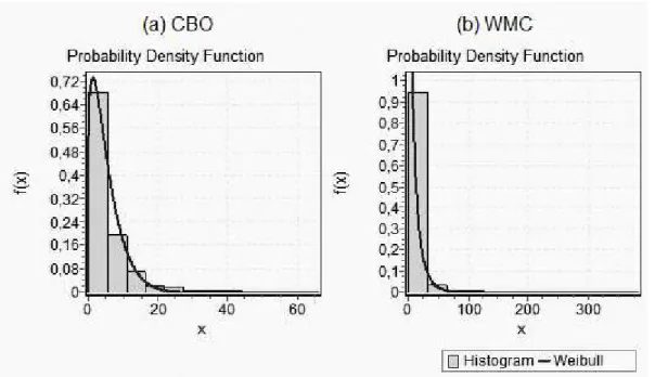
According to the classification schema suggested by Foss et al. [2011], the metric hasheavy−tailed distributionwhen the best distribution of a particular measure is one of the following: W eibull, Lognormal, Cauchy, P areto, or Exponential. We decided to use Weibull distribution because its versatility and relative simplicity. Weibull has two main probability distribution functions: (i)probability density function(pdf) – f(x), and (ii)cumulative distribution function (cdf) – F(x). The first function expresses the probability the random variable takes a value x. On the other hand, cdf expresses the probability the random variable takes a value less than or equal to x [Mathwave, 2015]. These functions have parametersα and β, defined by equations (Eq1) and (Eq2):

f x(x) =P(X =x) = α

β(x/β)

α₋1

e−(x β

α₎

, α >0, β >0

F w(x) =P(X ≤x) = 1−e−(x β)

α

(45)

3.2. Comparative Study ₂₅

The parameter β is called by scale parameter. Increasing the value of β has the effect of decreasing the height of the curve and stretching it. The parameter α is called by shape parameter. If the shape parameter is less than 1, Weibull is a heavy-tailed distribution [Mathwave, 20015]. A heavy-heavy-tailed distribution means that a small number of entities have high values and a large number of cases have low values. In this distribution, the mean is not representative [Alves et al., 2010; Ferreira et al., 2012; Mathwave, 2015].

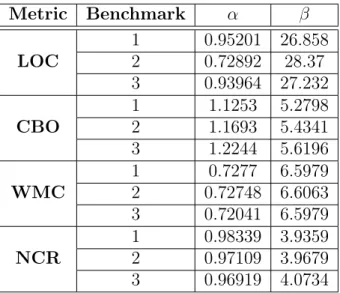
Table 3.3 presents the values of α and β for each metric and benchmark. For example, LOC has values of α = 0,95201 and β = 26,858 for Benchmark 1. Based on the analysis of the parameter α, we can observe that the metrics LOC, WMC, and NCR follow a heavy-tailed distribution. According to Table 3.3, CBO does not follow a heavy-tailed distribution for FOP-based SPL implementations because it presents α

values higher than 1. By analyzing the parameters values, we can be more confident about the metric distribution because, in some cases (e.g., depending of the scale), the plotted graph may give the wrong impression that the metric follows a heavy-tailed distribution.

Table 3.3: Weibull Values for Each Metric per Benchmark

Metric Benchmark α β

LOC

1 0.95201 26.858 2 0.72892 28.37 3 0.93964 27.232

CBO

1 1.1253 5.2798 2 1.1693 5.4341 3 1.2244 5.6196

WMC

1 0.7277 6.5979 2 0.72748 6.6063 3 0.72041 6.5979

NCR

1 0.98339 3.9359 2 0.97109 3.9679 3 0.96919 4.0734

3.2.3 Derived Thresholds

(46)

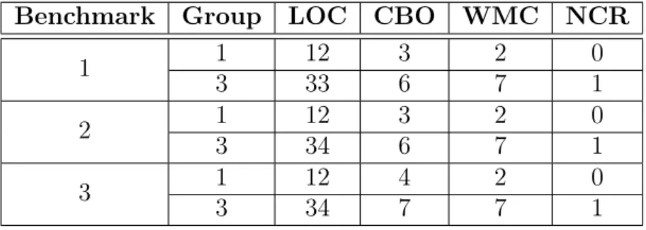
the values that represent the percentages are shown. This presentation strategy is also applied to Ferreira’s method, because the range of values of group 2 is equals to the ranges of groups 1 and 3. In addition, although Ferreira’s method definition does not provide how to extract the three groups, we extracted them by our own knowledge about the method. The three groups have 50% (good), 25% (regular) and, 25% (bad) of data, respectively.

Tables 3.4, 3.5, and 3.6 present the obtained values from the three methods, respectively. We present in separate tables because each method has a different output. These tables should be read as follows. The first column represents the benchmarks and the second column indicates the different labels in the case of Alves’s and Ferreira’s methods. The other columns determine the thresholds of LOC, CBO, WMC, and NCR, respectively. For example, Alves’s method defined labels as: low

(0-70%), moderate (70-80%), high (80-90%), and veryhigh (90-100%). These labels are represented for CBO by the intervals 0-8, 9-12, 13-20, and >21, respectively in Benchmark 1.

Table 3.4: Threshold Values from Alves’s Method

Benchmark Percentage LOC CBO WMC NCR

1

70 92 9 14 1

80 151 13 31 2

90 252 21 58 4

2

70 127 13 25 1

80 221 19 45 1

90 328 24 75 5

3

70 192 18 40 1

80 293 22 58 1

90 442 29 84 7

Table 3.5: Threshold Values from Ferreira’s Method

Benchmark Group LOC CBO WMC NCR

1 1 12 3 2 0

3 33 6 7 1

2 1 12 3 2 0

3 34 6 7 1

3 1 12 4 2 0

(47)

3.2. Comparative Study ₂₇

Table 3.6: Threshold Values from Oliveira’s Method

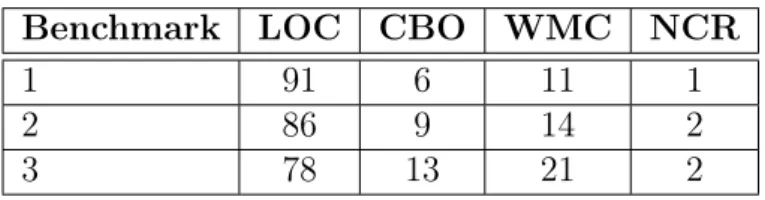
Benchmark LOC CBO WMC NCR

1 91 6 11 1

2 86 9 14 2

3 78 13 21 2

It should be observed that there is a difference between the thresholds from the same method (varying the benchmark) and between methods. The variation was sharper in the case of Alves’s method. This variation happens because the smallest (22 LOC) and the largest (37,247 LOC) SPLs have the same weight (step 4 of Alves’s method description). Hence, a higher variation across benchmarks was observed in the case of metrics with high correlation with size. We did not have a high variation in the case of NCR, which has low correlation with size (LOC). The other methods do not correlate metrics and do not weight metrics by the number of systems. Then, in almost all cases, the thresholds remained the same or have a slight growth in the system size. A peculiar case occurred in Oliveira’s method (Table 3.6), in which LOC had a small decrease. This decrease is probably impacted by the penalties applied to derive metric thresholds. We did not expect for it because with larger SPLs and consequently lager class it was expected higher thresholds. It does not mean a problem only a particularity of such metric for this method.

(48)

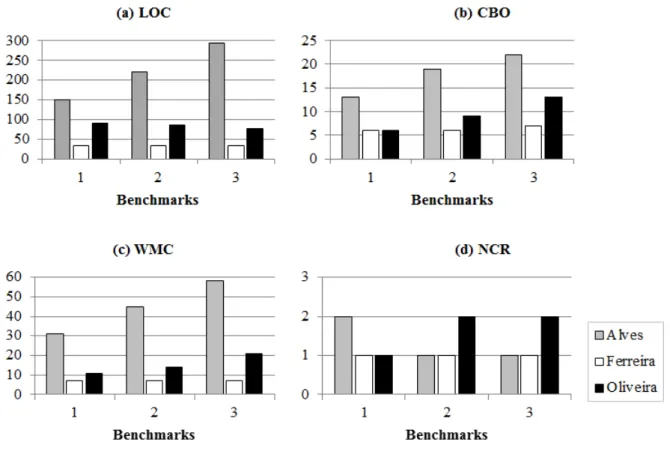
Figure 3.1: Metric Thresholds Side by Side

By analyzing the derived thresholds and considering the correlation of the metrics with LOC (Section 3.2.1), it is possible to see that Alves’s method has undergone a major change in its behavior. This major change is probably, due to the method cor-relate LOC to calculate thresholds. With respect to Ferreira’ and Oliveira’s methods, it is not possible to observe a clear change in their behavior like Alves’s method.

(49)

3.3. Desirable Points of Threshold Derivation Methods ₂₉

To illustrate this point, the threshold 6 to CBO defined by Oliveira’s method for Benchmark 1 has 639 outliers out of 2,700 entities. This number of outliers represents 23.67% of the entities. We consider that this percentage is not reasonable, as we do not want a very large number of outliers. Based on this observation, we can conclude that: (i) this calculation is extremely dependent from the benchmark quality to the three methods and (ii) Alves’s method is more rigid to define thresholds than the other methods. Considering these two points, we believe Alves’s method fared better with the majority of the analyzed metrics, especially with the ones highly correlated with LOC.

It is clear that some metrics are correlated to others and this is expected. How-ever, we considered that correlating metrics to calculate thresholds may not be a good practice, when this correlation is low. Since it is not always easy to know if a met-ric correlates with other metmet-rics; it might be better to not correlate metmet-rics to derive thresholds. In the case of the distribution of the software metrics, the three meth-ods seem to work well with heavy-tail distributions. Even if the distribution is not heavy-tailed, the three methods presented similar derived thresholds.

3.3 Desirable Points of Threshold Derivation

Methods

(50)

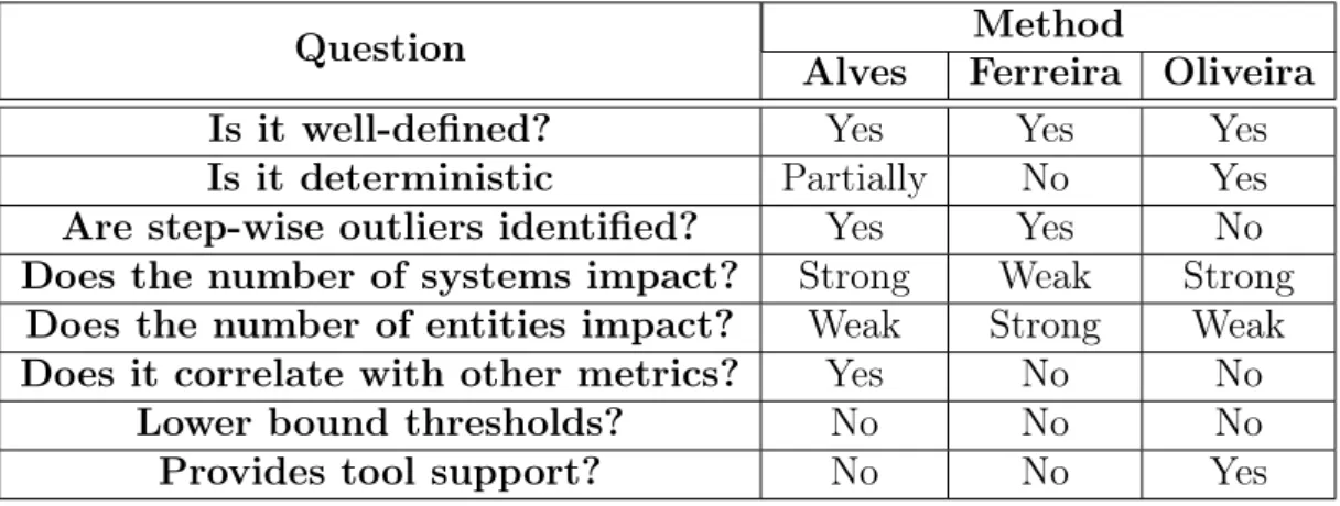
Table 3.7: Comparative Evaluation of the Method for Calculating Thresholds

Question Method

Alves Ferreira Oliveira Is it well-defined? Yes Yes Yes

Is it deterministic Partially No Yes

Are step-wise outliers identified? Yes Yes No

Does the number of systems impact? Strong Weak Strong

Does the number of entities impact? Weak Strong Weak

Does it correlate with other metrics? Yes No No

Lower bound thresholds? No No No

Provides tool support? No No Yes

Well-defined and Deterministic – We consider well-defined methods when it is possible to define steps based on the method description. As we did it for the three methods, we considered all these three methods well-defined. If we replicate this study, are the results going to be exactly the same? Alves’s method is well-defined, but the chosen percentage can vary. Therefore, we considered it as partially deterministic. In the case of Ferreira’s method, it does not describe how the three groups should be extracted and, so, this subjectiveness makes it well-defined, but not deterministic. Oliveira’s method is highly deterministic and well-defined. If someone uses the same input, the same results are expected to be obtained.

Number of Systems and Entities - Thresholds are extracted from software entities (e.g., features, modules and classes). Therefore, the main information used for calculating thresholds is expected to be metrics collected from these entities instead of the number of systems, for example. Although the number of systems can be considered important in terms of representativeness, we believe that the number of entities is more important. Hence, a method is expected to derive thresholds weakly dependent on the number of systems and strongly dependent on the number of entities. Alves’s method calculates thresholds by using, essentially, the number of systems. Both Ferreira’s and Oliveira’s methods use the number of entities to derive thresholds. However, Oliveira’s method uses the median of entities of the systems. Therefore, Alves’s and Oliveira’s methods can be considered as strongly dependent to the number of systems and Ferreira’s method as strongly dependent to the number of entities.

(51)

3.4. Threats to Validity ₃₁

does not make explicit whether or not to weight measurements by LOC. The other two methods do not consider the correlation of metrics with LOC. As explained in the end of Section 3.2.1, we believe that, in the general case, it is better to not correlate metrics to calculate thresholds.

Lower Bound Thresholds and Tools Support- Thresholds are often used to filter upper bound outliers. However, in some cases, it may make sense to identify lower bound outliers. For instance, classes with low values of LOC can be an indicative of the Lazy Class code smell [Fowler et al., 1999]. A Lazy Class is defined as a class that knows or does too little in the software system [Fowler et al., 1999]. None of analyzed methods calculate lower bound thresholds. Tool support is not essential, but it can facilitate the use of a method because it easier it’s systematic application. Among the analyzed methods, we only found a tool to support the Oliveira’s method [Oliveira et al., 2014].

Given the answer of these question we think that it is desirable that a method should: (i) be well-defined and deterministic; (ii) derive thresholds in a step-wise for-mat; (iii) be weakly dependent on the number of systems; (iv) be strongly dependent on the number of entities; (v) not correlate metrics; (vi) calculate upper and lower thresholds; (vii) provide representative thresholds independent of metric distribution, and (viii) provide tool support.

3.4 Threats to Validity

Even with the careful planning, this research can be affected by different factors which, while extraneous to the concerns of the research, can invalidate its main findings. Actions to mitigate their impact on the research results are described below.

SPL Repository – We followed a careful set of procedures to create the SPL repository and build the benchmarks. As the number of open source SPLs found is limited, we could not derive a repository with a larger number of SPLs. This limitation has implication in the amount of analyzed entities, which is particularly relevant to NCR. This factor can influence the defined thresholds as the number of entities for NCR analysis is further reduced. In order to mitigate this limitation, we created different benchmarks for comparison of the derived thresholds.

(52)

to extract the three groups required us to define three groups with approximately 50% (good), 25% (regular) and, 25% (bad) of data, respectively, totalizing the 100%. We know that Ferreira’s method needs a graphic analysis, but to make it more systematic we decided to derive the thresholds with those percentages. Since the other methods are full or partially deterministic, we did not have this problem with them.

Measurement Process – The SPL measurement process in our study was automated based on the use of existing tooling support. However, as far as we are con-cerned, there is no existing tool defined to explicitly collect metrics in FeatureHouse (FH) code. Therefore, the SPLs developed with this technology had to be transformed into AHEAD code. This transformation was made changing the composer of FH to the composer of AHEAD. There are reports in the literature justifying that this trans-formation preserves all properties of FH [Apel et al., 2009]. We also reduced possible threats by performing automated tests with a few SPLs. In fact, we observed all software proprieties were preserved after the transformation.

Tooling Support and Scoping– The computation of metric values and metric thresholds can be affected by the tooling support and by scoping. Different tools implement different variations of the same metrics [Alves et al., 2010]. To overcome this problem, the VSD tool [Abilio et al., 2014] was used both to collect the metric values and to identify God Class instances. The tool configuration with respect to which files to include in the analysis (scoping) also influences the computed thresholds. For instance, the existence of test code, which contains very little complexity, may result in lower threshold values [Alves et al., 2010]. On the other hand, the existence of generated code, which normally has very high complexity, may result in higher threshold values [Alves et al., 2010]. As previously stated, for deriving thresholds, we removed allsupplementary code(e.g., generated code and test cases) from our analysis.

3.5 Final Remarks

This chapter discussed the calculation of representative thresholds in the light of three methods to derive metric thresholds. These methods were described and compared using as input data metrics collected from 33 SPLs. We believe that the methods were reasonable evaluated because we provided a comparison with respect to: (i) three dif-ferent benchmarks, (ii) metrics with difdif-ferent distributions, (iii) metrics with difdif-ferent degrees of correlation with LOC, and (iv) an analysis of the derived thresholds.

(53)

3.5. Final Remarks ₃₃

recent ones (to exclude duplicates). In addition, we applied two refinements to extract Benchmarks 2 and 3. These two refinements consist of keeping only SPLs with more than 300 and 1,000 LOC, respectively. Providing the benchmarks as input for the methods, we observed that Alves’s method is a little more sensitive to the benchmark quality. It happened because this method weights each SPL by LOC and SPLs with different sizes receive the same weight.

Regarding distribution of the metrics used in this study, the metrics LOC, WMC, and NCR have heavy −tailed distributions. In spite of following a different distri-bution, CBO apparently did not present a different behavior of the other metrics. Although we have a small sample, the methods seemed to behave well with different distributions. Regarding metrics correlation, we noticed that Alves’s method correlates metrics to derive thresholds. As can be seen in Section 3.2.1, correlating metrics can be danger, when we have metrics with low correlation. The other methods did not correlate metrics and, hence, this problem did not impact them.

In order to provide reliable outcomes, we analyzed the thresholds individually. We considered that Alves’s method was better in the individual evaluation because it presented more representative thresholds given the inputs for three out of four metrics. In addition, the thresholds are higher compared to the other methods. It resulted in a smaller number of outliers compared to the number of outliers detected by the other methods. On the other hand, Alves’s method seems to be more instable when metrics have low correlation with LOC.

(54)

(55)

Chapter 4 The Proposed Method

Based on the comparison of methods presented in the previous chapter, we see the opportunity to propose a method to derive thresholds with the strangeness and avoiding the weaknesses of the compared methods. However, this chapter proposes a method to derive thresholds based on the eight desirable points described in the previous Chapter. Section 4.1 presents the proposed method. Section 4.2 describes how we believe that our method addresses the eight desirable points. Section 4.3 presents the tool to support the method. Section 4.4 provides an example of use of the proposed method using a Software Product Line (SPL) benchmark. Section 4.5 presents some threats to validity to the proposed method and it example of use. Section 4.6 summarizes this chapter.

4.1 Method Description

We propose a method with 5 well-defined steps. With the proposed method, we try to get the best of each compared method avoiding the points that we saw are not adequate for methods to derive thresholds, such as, metrics’ correlation. Figure 4.1 summarizes the 5 steps of the proposed method. Each step is described as follows.

1. Metric extraction: in the first step, metrics have to be extracted from a

benchmark of software systems. For each system, and for each entity belonging to the system (e.g., class), we record a metric value. The metric value of each entity of the entire benchmark must be in the same file, such as a spreadsheet. Each column represents a metric and each row represents an entity.

2. Weight ratio calculation: for each entity, we compute the weight percentage within the total number of entities in the second step. That is, we divide the entity weight by the total number of entities and, then, it is multiplied by one hundred. All

(56)

36 Chapter 4. The Proposed Method

Figure 4.1: Summary of the Method Steps

entities have the same weight and the sum of all entities must be 100%. As an example, if one benchmark has 10,000 entities, each entity represents 0.01% of the overall (0.01% x 10,000 = 100%).

3. Sort in ascending order: we sort the metric values in ascending order and take the maximal metric value that represents 1%, 2%, . . . , 100%, of the weight. This step is equivalent to computing a density function, in which the x-axis represents the weight ratio (0-100%), and the y-axis the metric scale. For instance, all entities that WMC value is 4 must come first that all metrics which WMC value is 5.

4. Entity aggregation: we aggregate all entities per metric value in the step. This aggregation is equivalent to computing a weighted histogram (the sum of all bins must be 100%). As an example, if we have four entities with WMC value of 4 and each entity representing 0.01%, it corresponds to 0.04% of all entities.

A benchmark-based method to derive metric thresholds

A BENCHMARK-BASED METHOD TO DERIVE

GUSTAVO ANDRADE DO VALE

A BENCHMARK-BASED METHOD TO DERIVE

METRIC THRESHOLDS

Orientador: Eduardo Magno Lages Figueiredo

Belo Horizonte

GUSTAVO ANDRADE DO VALE

A BENCHMARK-BASED METHOD TO DERIVE

METRIC THRESHOLDS

Advisor: Eduardo Magno Lages Figueiredo

Belo Horizonte

Acknowledgments

Resumo

Abstract

List of Figures

List of Tables

Contents

Chapter 1

Introduction

1.1

Motivation, Problem Description, and Goal

1.2

Methodological Procedures and Contributions

1.3

Dissertation Outline

Chapter 2

Background

2.1

Software Product Lines

2.2

Software Metrics

2.3

Literature Review Protocol

2.4

Types of Methods to Derive Thresholds

2.4.1

Thresholds Derived from Programming Experience

2.4.2

Thresholds Derived from Metric Analysis

2.4.3

Methods for Characterizing Metric Distributions

2.5

Key Points of Methods to Derive Thresholds

2.5.1

Well-defined Methods

2.5.2

Consider the Skewed Distribution of Software Metrics

2.5.3

Benchmark-based

2.6

Methods to Derive Thresholds that Fit the Key

Points

2.7

Final Remarks

Chapter 3

A Comparison of Methods to

Derive Metric Thresholds

3.1

SPL Benchmarks

3.2

Comparative Study

3.2.1

Correlation with LOC

3.2.2

Distribution of Software Metrics

3.2.3

Derived Thresholds

3.3

Desirable Points of Threshold Derivation

Methods

3.4

Threats to Validity

3.5

Final Remarks

Chapter 4

The Proposed Method

4.1

Method Description