Treatment of geophysical data as a
non-stationary process
MARCUS P.C. ROCHA and LOURENILDO W.B. LEITE Department of Mathematics
Department of Geophysics, Graduate Course in Geophysics Federal University of Pará, Brazil
E-mail: mrocha@ufpa.br / lwbleite@ufpa.br
Abstract. The Kalman-Bucy method is here analized and applied to the solution of a specific filtering problem to increase the signal message/noise ratio. The method is a time domain treatment of a geophysical process classified as stochastic non-stationary. The derivation of the estimator is based on the relationship between the Kalman-Bucy and Wiener approaches for linear systems. In the present work we emphasize the criterion used, the model with apriori information, the algorithm, and the quality as related to the results. The examples are for the ideal well-log response, and the results indicate that this method can be used on a variety of geophysical data treatments, and its study clearly offers a proper insight into modeling and processing of geophysical problems.
Mathematical subject classification:49N45, 54H20, 74H50, 93C05.
Key words:stochastic process, Kalmann-Bucy filter, deconvolution, state space.
1 Introduction
A seismic signal represents the transient response of the Earth to excitation due to natural phenomena, such as eathquakes, or due to artificial sources as used in geophysical exploration, and it results in non-stationaty signals in noise. The aim of the seismic processing is to improve conditions for the interpretation of registered data. A detailed representation of a seismic signal requires a rather complicated formulation, and the processing uses a group of techniques based on stochastic properties of the model.
Two types of mathematical methods for data treatment can be used to represent a seismic signal: deterministic and stochastic. The deterministic method consists of using physical theories of wave propagation involving solutions of integral and differential equations satisfying contour and initial conditions. The stochastic method takes the statistical description of time series for the expressions of dynamic laws as statistical facts.
In this this work we apply Kalman-Bucy method to treat geophysical data. For this, we analyze the a priori necessary conditions to transform the governing integral equation of the first kind to linear and to non-linear ordinary differential equations using the state space technique. We reinforce the understanding of the limitations of the procedure for the separation of the signal message from noise in the time domain, and we make use of the property that geophysical data represent realizations that are strongly white non-stationary stochastic processes. The importance of the Kalman method stems both conceptually in the formu-lation of the solution of a fundamental geophysical problem, and also from its versatility and applicability as an adaptative data processing. Some basic geo-physical references followed in the present topic are Robinson (1999), Mendel (1990, 1983), Crump (1974), Bayless and Brigham (1970) and Van Trees (1968). Engeneering applications have available a heavy machinery on this subject for real-time applications, and to name a few we count with Kailath (1981), Chui and Chen (1987), Candy (1987) and Brown and Hwang (1996).
2 The Wiener-Kolmogorov problem
For motivation, consider the classical optimum time-invariant operator obtained by using the criterion of minimum error variance between the actual output,x(t )ˆ , and the desired output,x(t ). The model is expressed by
z(t )=x(t )+v(t ), (1)
wherez(t )is the measurement, andv(t )is the additive noise. The filter operation is described by the convolution integral
ˆ
x(t )=
+∞
−∞
whereh(t )is the unknown time-invarint operator that is constrained to satisfy the commonly referred as the Wiener-Hopf integral equation
φxz(t )=
+∞
−∞
hw(τ )φzz(t−τ )dτ, (3)
whereφxz(t )andφzz(t )are, respectively, the admitted known theoretical stochas-tic crosscorrelation and autocorrelation functions. It this basic formulation,x(t )
andv(t )are stationary random processes, and together withz(t ),h(t ),φxz(t ) andφzz(t )are real function, continuous, time unbound, and convergent.
To specify the optimun (not necessary best) operator it is necessary to solve the integral equation 3. This situation becomes more difficult as the complexity of the problem increases, and when it does not satisfy strictly the characteristics of the geophysical problem that we have in hands that has for description to be non-stationary.
The present problem, with respect to the non-stationarity and to the data win-dow, does not satisfy the principles underlined by the convolution integral. For this reason the equation is rewritten in the form of a moving average according to the commonly referred to as the Wiener-Kolmolgorov problem. The general-ization corresponds to the integral of the Booton type, and it is expressed by the matrix integral equation
φ
xz(t, σ )=
t
t0
h(t, τ )φ
zz(τ, σ )dτ, (4)
for
ˆ
x(t )=
t
t0
h(t, τ )z(τ )dτ, (5)
wherex(t )ˆ is the estimated actual output, andh(t, τ )is the corresponding desired optimum time-variant operator. Again, the criterion used is the minimization of the residue covariance expressed as
I (h)=E{[ ˆx(t )−x(t )]2}, (6) that results in the normal equations between the deviations and the observations,
Equation (4) carries the inherent difficulties of the integral equation of the first kind. On the other hand, it is the natural representation for the treatment of mul-tidimensional non-stationary random processes, it includes finite observations, and it admits time-variant estimates. The problem as written under equation (4) can be classified as an inversion identification problem, and this setting is in general non-linear and ill-posed in the sense of Hardamard; nevertheless, the solvability and the stability are achieved by a priori information. For a practical solution, Kalman and Bucy (1961) proposed conversion of this integral to linear and non-linear ordinary differential equation, which results to be more adapt-able to numerical calculations. The optimum estimator is completely specified and synthesized with the a priori information on the forward model, and on the statistics of the components.
3 The state space solution
The formulation begins by expressing the original problem as an ordinary dif-ferential equation of ordemN −1
N−1
n=0
an(t )
dny(t )
dtn =w(t ), (a1=1) (8)
The transformation to the state variablexn(t )andx˙n(t )is achieved by substituting the higher derivatives ofy(t )in the form:
x1=y, x2= ˙y, x3= ¨y, ..., xN =yN−1 (9) ˙
x1=y, x2=x3,x˙3=x4, ...,x˙N−1=xn (10) ˙
xn = −(anx1+an−1x2+...+a1xn)+w (11) The resulting dynamic state equation in the general (continuous, time-variant) compact form are:
˙
x(t )=F (t )x(t )+G(t )w(t ), (system), (12)
F (t ),G(t )andH (t )are matrices with variable elements int;w(t )is the forcing function that generates the state;z(t )is the selected form for the output given by the structure of the matrixH (t );v(t )is the addtive noise present (Ogata, 1995; Kuo, 1992).
For the development of the estimator, it is necessary to define the apriori general stochastic properties for the processes,z(t ),w(t )andv(t ), and the natural description takes into consideration average values and variances. The table of a priori conditions is formed by the autocorrelations of white noise, and by mull crosscorrelations in the window of definition of the governing integral equation, and they are:
E{w(t )} =0, φ
ww(t, τ )=E{w(t )w T(τ )
} =W (t )δ(t−τ ), (14)
E{v(t )} =0, φ
vv(t, τ )=E{v(t )v T
(τ )} =V (t )δ(t−τ ), (15)
φ
wz(t, τ )=E{w(t )z T(t )
} =0, φ
wv(t, τ )=E{w(t )v T(τ )
} =0, (16)
φ
xv(t, τ )=E{x(t )v T(t )
} =0, φ
wx(t, τ )=E{w(t )x T(τ )
} =0. (17)
Observe that delta functions multiplyingW (t )andV (t )define the autocorre-alation as diagonal matrices. These relations represent the strong properties of the model, and they do not establish a specific distribution, but only a structure. For instance, we chose red noise for our example, and the theory can be modi-fied to account for such. F (t ),G(t ),H (t ),w(t ),φ
vv(t ),V (t )andW (t )are real, continuous, time unbound, and convergent.
The philosophy behind this transformation is to substitute the state equations into the integral equations, and apply the premises. We present only the main critical steps to point out where the necessary properties are inserted.
We look at the transformation of the integral (4) by frist calculating the correla-tionsφ
zz(t, σ )andφxx(t, σ ). With this aim, we initiate with the definition of the crosscorrelation,φ
xz(t, σ ), and insert the dynamic equation of the measurement; that is
φ
xz(t, σ )=E{w(t )z T(σ )
With the a priori condition of (14)
φ
xz(t, σ )=φxx(t, σ )H
T(t ). (19)
The autocorrelationφ
zz(t, σ )is in a similar manner given by the expression
φ
zz(t, σ ) = E{z(t )z T
(σ )}
= E{[H (t )x(t )+v(t )][H (σ )x(σ )+v(σ )]T}.
(20)
With the a priori conditions (13) and (14), the above is further simplified to
φ
zz(t, σ )=H (t )φxx(t, σ )H T
(σ )+V (t )δ(t−σ ). (21)
Substituting (16) in the original equation (4) results in that
φ
xx(t, σ )H T(σ )
=
t
t0
h(t, τ )φ
zz(τ, σ )dτ. (22)
Equation (18) and (19) are intermediate relations to express the autocorrelations
φ
zz(t, σ )andφxx(t, σ ), and they will be simplified in the next section and applied to original integral equation (4).
3.1 Inserting the state equation into the stochastic model
System equation (10) is inserted through the autocorrelation as an intermediate step for obtaining the differential equation for state estimate. For this purpose, it is necessary to differentiateφ
xx(t, σ ), and therefore
∂φ
xx(t, σ )
∂t =E
dx(t )
dt x
T
(σ )
=E{[F (t )x(t )+G(t )w(t )]xT(σ )}. (23)
Applying the a priori condition (14) gives us
∂φ
xx(t, σ )
∂t =F (t )φxx(t, σ ). (24)
Multiplying both sides byHT(σ ), we have that
∂φ
xx(t, σ )
∂t H
T(σ )
=F (t )φ
xx(t, σ )H
And transposing (19) to (20) we arrive at
∂φ
xx(t, σ )
∂t H
T
(σ )=
t
t0 F (t )h
zz(τ, σ )dτ. (26)
Differentiating equation (19) we obtain,
∂φ
xx(t, σ )
∂t H
T(t )
=h(t, t )φ
zz(t, σ )+
t
t0
∂h(t, τ )
∂t φzz(τ, σ )dτ. (27)
Multiplying both sides of equation (18) byh(t, t ), it follows that
h(t, t )φ
zz(t, σ )=h(t, t )H (t )φxx(t, σ )H T
(σ ). (28)
Substituting (19) into (24) we obtain
h(t, t )φ
zz(t, σ )=
t
t0
h(t, t )H (t )h(t, τ )φ
zz(τ, σ )dτ. (29) Substituting (26) and (23) into (24), and rearranging terms we find that
t
t0
−F (t )h(t, τ )+h(t, t )H (t )h(t, τ )+∂h(t, τ ) ∂t
φ
zz(τ, σ )dτ =0. (30) Under the condition of non-vanish ofφ
zzin the integration interval, we conclude that
∂h(t, τ )
∂t =F (t )h(t, τ )−h(t, t )H (t )h(t, τ ). (31)
3.2 The gain matriz and the solution of the integral equation
In this section we define the gain matrix of the problem, and we arrive at the solution of the integral equation (4), using relations (28), (16) and (18) defined in the previous section, maintaining the validity conditions of the solution in the interval(t0, t ).
The application of Leibnitz rule to differentiate equation (5) is an intermediate step for the differential of the estimated valuex(t )ˆ , and it is given by
dx(t )ˆ
dt =h(t, t )z(t )+
T
t0
∂h(t, τ )
∂t z(τ )dτ. (32)
Substituting equation (28) in the above equation and rearranging terms, we obtain
dx(t )ˆ
dt =h(t, t )z(t )+
t
t0
F (t )h(t, τ )z(τ )
−h(t, t )H (t )
t
t0
h(t, τ )z(τ )dτ,
(33)
where we use equation (5) to write
ˆ˙
x(t )=F (t )x(t )ˆ +h(t, t )[z(t )−H (t )x(t )ˆ ]. (34)
This is an intermediate result for the state estimate in terms of known function and of the apriori conditions. It is still necessary to arrive at an explicit expression for
h(t, t ), which means that the values of definition for the operator is coincident with that of the data,τ =t. In this special position, we identifyh(t, t )=K(t ), andK(t ) is the commonly referred to as the gain matriz, and it contains the maximum extension of data involved in the integral equation operation. We now have the integral equation (4) transformed to the state differential equation rewritten in the form.
ˆ˙
x(t )=
F (t )−K(t )H (t )
ˆ
x(t )+K(t )z(t ), (35)
and its solution is given by knowingK(t ).
G(t ), H (t ), V (t ) andW (t ), in the next section. In equation (4) the autocor-relation represents the data model, and with (11) we write it as; φ
zz(t, σ ) =
φ
yy(t, σ )+φyv(t, σ )+φvy(t, σ )+φvv(t, σ ), with null crosscorrelation. The measurement model is made asy(t ) = H (t )x(t ), and also condition (13) ap-plies. In equation (4) the crosscorrelationφ
xz(t, σ )represents the measurement, and we makez(t )→ y(t ), andφ
xz(t, σ ) → φxy(t, τ ). With these conditions imposed on equation (4) it takes the form
φ
xy(t, σ )−
t
t0
h(t, τ )H (τ )φ
xy(τ, σ )dτ =h(τ, σ )V (σ ). (36) For the caseσ =t, we have that the integral is the estimate forφ
xy(t, σ ), them
φ
xy(t, t )− ˆφxy(t, t )=K(t )V (t ). (37) The measurement model gives thaty(t ) = H (t )x(t ). Also, φ
xy(t, t ) =
φ
xx(t, t )H
T(t ). We define φ
xx(t, t ) = φxx(t, t ) − ˆφxx(t, t ). With these considerations, equation (34) given the result
P (t )HT(t )=K(t )V (t ). (38)
3.3 The Ricatti differential equation
We continue with the analyzes of the error autocorrelation matrix defined by
P (t )=E{x(t )xT(t )}. (39)
The idea is to differentialP (t )and to apply the premises. Therefore,
˙
P (t )=E
dx(t )
dt x
T
(t )
+E
xT(t )x(t ) dt
. (40)
The next steps are to expand both of these terms, with the system error defined by
Substituting equation (32), (10) and (11) in (37), and rearranging terms, we find that
x(t )˙ = [F (t )−K(t )H (t )]x(t )−K(t )v(t )+G(t )w(t ). (42)
The tarnsition matrix ofx(t ),(t, t0), is defined as
(t, t0)=F (t )−K(t )H (t ). (43)
With this definition, the solution of the differential equation (38) is given by
x(t ) =(t, t0)x(t0)−
t
t0
(t, τ )K(τ )v(τ )dτ
+
t
t0
(t, τ )G(τ )w(τ )dτ,
(44)
Using equation (38), we can expand the frist term of equation (36) in the following form:
E
dx(t )
dt x
T(t )
= [F (t )−K(t )H (t )]E{x(t )xT(t )} (45)
We observe that to solve equation (41) it is necessary to find the crosscorrelations
φ
vx(t, t )andφwx(t, t ). Frist, we consider the expression
φ
vx(t, t )=E{v(v)x T(t )
}. (46)
This point is important because we can not consider a priori conditions of non-correlation due tox(t ). Substituting equation (40) in (42), and writing it with
T(t, t0)=(t, t0)we obtain that
φ
xx(t, t )=(t, t0)E{v(t )x T(t )
} −
t
t0
E{v(t )vT(τ )}KT(t )T(t, τ )dτ
(47)
Bringing the expectation inside the integral, and applying the table of a priori conditions of non-correlation, it simplifies to
φ
vx(t, t )= −
T
t0
Substituting equation (13), it results in that
φ
vx(t, t )= −
t
t0
V (t )KT(τ )T(t, τ )δ(t−τ )dτ (49)
The integral (45) hastfor upper limit. The unitary impulso can be described by the even rectangular function (1/T )(Barton, 1999):
δ(t )= lim T→0
1 T , 1 T 1 T = (50)
The integration covers only half of the interval of symmetry of δ(t ). Also, for the problem under study the integrand is to be causal, and(t, t )=I. Applying these conditions, equation (45) simplifies to
φ
vx(t, t )= − 1 2V (t )K
T
(t ). (51)
In a similar procedure we determineφwx(t, t )by the following relations
φ
wx(t, t )=E{w(t )x T(τ )
}, (52)
φ
wx(t, t )=
t
t0
E{w(t )wT(τ )}GT(t )T(t, τ )dτ, (53)
to obtain
φ
wx(t, t )= 1 2W (t )G
T(t ). (54)
Substituting equation (48) and (51) in (41), under the established a priori condi-tions, and thatP (t )=E{x(t )xT(t )
}we obtain
E
dx
dt x
T(t )
= [F (t )−K(t )H (t )]P (t )
+1
2K(t )V (t )K T(t )
+ 1
2G(t )W (t )G T(t ).
(55)
In an analogous form, we obtain for the second term of the expression (36)
E
x(t )dx
T
dt
= [F (t )−K(t )H (t )]TP (t )
+12K(t )V (t )KT(t )+ 1
2G(t )W (t )G T(t ).
Adding equation (52) and (53) we have for equation (36) that
˙
P (t )= [F (t )−K(t )H (t )]P (t )+P (t )[F (t )−K(t )H (t )]T + (57)
Finally, by substitutingK(t )from (35) we arrive at the non-linear error covari-ance Ricatti natrix differential equation
˙
P (t ) =F (t )P (t )+P (t )FT(t )−P (t )HT(t )R−1(t )H (t )P (t )
+G(t )Q(t )GT(t ). (58)
This system of coupled equations, (55), (35) and (32) compose the solution of the transformation. The functionP (t )andK(t )are real, continuous, time non-unbounded, and convergent. Our final goal is the application to synthetic and to real data, and we describe next the model that server as an axample (Rocha, 1998).
4 Model construction and data processing
We present the model in a scalar form as by square waves, and this is meant to correspond to ideal situations in geophysics of measurements. The signal mes-sagex(t )is measured in the presence of the noise,v(t ), with a priori conditions of zero averege and varianceσa2. In this filtering simulation we look for recov-ering the signal message in noise, what represents a frist step in the search for the function that describes the geology of the medium.
4.1 Simulated example
This process is based on the convolution of the random function,s(t ), represent-ing the simple reflectivity of the medium, with a Heaviside function,u(t ), to generate the message,x(t ), and this is expressed as:
x(t )=s(t )∗u(t ), (without noise), (59)
Continuing with the model description, we table the white stochastic properties as:
E{x(t )} =0, φxx(t1, t2)=E{x(t1)x(t2)} =λσa2δ(t1−t2), (61)
E{w(t )} =0 φww(t1, t2)=E{w(t1)w(t2)} =λσa2δ(t1−t2), (62)
E{v(t )} =0 φvv(t1, t2)=E{v(t1)v(t2)} =σv2δ(t1−t2). (63) Comparing the above premises with the general dynamic Kalman equations, and adjusting the free variables ast=t1,τ =t2, we have conveniently that
Q(t )=Q=λσa2, V (t )=V =σr2. (64) For the solution of the problem it is necessary to define the state variables, and here they are selected in the following form:
x1(t )=x(t )=y(t ) x2(t )= ˙x1(t )= ˙x(t )=w(t ). (65) Comparing the above expressions with (10) and (11) we have that
˙
x1=0+w(t ) y(t )=x1(t ), (66)
and
F =0; G=1 H =1. (67)
The above relation give for the Ricatti matricial differential equation
˙
P (t )= −P (t )V−1(t )P (t )+W (t ). (68) And for the gain matrix
K(t )=P (t )HT(t )V−1(t ). (69) Substituing equation (61) and (62) in (66) and in (67), we obtain the differential equation for erro covariance in the scalar form,P (t )→p(t ), as given by
dp(t )
dt = −
p2(t ) σ2
v
and the corresponding gain by
K(t )= p(t ) σ2
v
. (71)
In the general solution for the Ricatti equation (55) in closed form appears the hiperbolic tangent function (Lewis, 1986; Davis, 1963),
K(t )=√γ
1−e2√γ t 1+e2√γ t
, γ =λσ
2 a
σ2 r
. (72)
With the gain function as defined above, we obtain the state differential equation for estimation in the desired scalar form:
dx(t )ˆ
dt = −
√γ
1−exp(−2√γ t )
1+exp(−2√γ t )
ˆ
x(t )
+√γ
1−exp(−2√γ t )
1+exp(−2√γ t )
z(t ).
(73)
The method used here for the numerical integration of the above equation is of the type Runge-Kutta, second order.
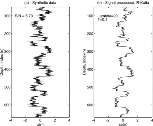
The synthetics in figure 1a obeys the principles of the adopted model, which is the convolution of the impulse response function of the medium,s(t ), with the Heaviside function,u(t ), resulting in a square wave,x(t ), with additive randon noise,v(t ).
The apriori conditions are displayed in figure 2, where the crosscorrelations between the desired signal,z(t ), and the noise,v(t ), shows to be small, although the theory requires it to be zero. The autocorrelation of the nessage,x(t ), and of the noise,v(t ), shows that the noise attends better the requirement of the theory. The distribuition is considered uniform in the data window.
100
200
300
400
500
600
-4 -2 0 2 4
Depth, Index(n)
xe(n)
(b) - Signal processed: R-Kutta
Lambda=20 T=0.1 100
200
300
400
500
600
-4 -2 0 2 4
Depth, Index (n)
z(n) (a) - Synthetic data
S/N = 5.73
Figure 1 – (a) Simulation of a sonic profile with the signal/noise ratio = 5.73 for the filter input. (b) A selected result of filtering withλ=20 Sampling intervalt=0.1.
-600 -400 -200 0 200 400 600
-0.2 -0.1 0 0.1 0.2
Index (m)
Azv
(a) - Crosscorrelation
-600 -400 -200 0 200 400 600
-1 -0.5 0 0.5 1
Index (m)
Axx e Avv
(b) - Autocorrelation
The discretizing is in the formt=nt. The depth is related to the indexn;t
is aquispaced, and it can represent any unit dimension of the SI system; namely, meter, kilometer, centimeter, second, etc. The signal message/noise ratio(S/N )
is simply calculated by
S
N =
1 N
N
i=1(xi− ¯x) 2 1
N
N
i=1(vi− ¯v)2
(74)
wherex¯ andv¯are the simples averege values.
Analyzing the performance of the processor in the several controlled experi-ments we observe that the time-variant operator is versatile, and it can be made more sophisticated to heve applicability in different situations of natural non-stationarity. The algorithm appears to be numerically convergent, but in all obtained results, we can see the influence of the transient response of the fil-ter operator characfil-terized by the symmetrical form of the hyperbolic tangent function.
4.2 Real data
The operationality of the Kalman filter was verified on real data with different characteristics from the synthetically simulated experiments. For this task we used a published log profile of clay volume measured in a well of the Maracaibo lake, Venezuela, as shown in figure 3. The initial stage consisted on the definition of each interval of the sequential windows without overlap for filter application
(t0 ≤ τ ≤ Ti), which begin at points where the variance is estimated. The sampling interval was fixed int =0.1 and the parameterλvaried asλ=10 andλ=20.
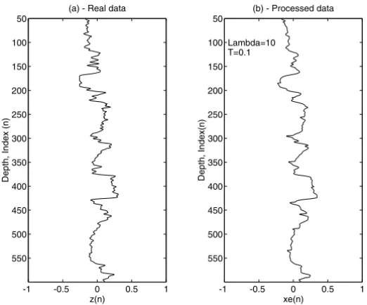
This data does not present itself with a clear descriptive noise component, which limits the simple comparison with the synthetic simulations. Figure 3 shows the satisfactory result demonstrated by the smoothing of noise in the data window.
5 Conclusions
50
100
150
200
250
300
350
400
450
500
550
-1 -0.5 0 0.5 1
Depth, Index (n)
z(n) (a) - Real data
50
100
150
200
250
300
350
400
450
500
550
-1 -0.5 0 0.5 1
Depth, Index(n)
xe(n) (b) - Processed data
Lambda=10 T=0.1
Figure 3 – (a) Data measured in a well of the Maracaibo lake, Venezuela. (b) The processed output using numerical procedure, with parameterγ = 10 and sampling spacingt =0.1.
The present method cam include sophistication through apriori knowledge in order to describe the model in more details, what can results in a gain in resolution in the processing of non-stationary data. On the other hand, the sophistication may represent a loss in the practical application of the algorithm.
On real data, the filter has the possibility of being structured in an interactive procedure with a continuous sweeping over the data using a group of control parameters. The display on the monitor screen serves the interpreter for making a systematic evaluation of the outputs.
6 Acknowledgments
REFERENCES
[1] G. Barton,Elements of Green’s Functions and Propagation, Oxford Science Publications. New York, USA, (1999).
[2] J.W. Bayless and E. Brigham,Application of the Kalman filter to continuous signal restoration, Geophysics,35(1) (1970), 2–23.
[3] R.G. Brown and P.Y.C. Hwang,Introduction to Randon Signals and Applied Kalman Filtering, John Wiley and Sons. New York, USA, (1996).
[4] J.V. Candy,Signal Processing. The Model-Based Approach, McGraw-Hill Book Company. New York, USA, (1987).
[5] C.K. Chui and G. Chem,Kalman Filtering. Springer-Verlag. Berlin, Germany, (1987). [6] N. Crump, A Kalman filter aproach to the deconvolution of seismic signals, Geophysics,
39(1) (1974), 1–13.
[7] M.C. Davis,Factoring the spectral matriz, IEEE Trans. on Automatic Control, AC-8 (1963), 196–225.
[8] T. Kailath, Lectures on Wiener and Kalman Filtering, Springer-Verlag. Berlin, Germany, (1981).
[9] R.E. Kalman and R.E. Bucy,New results in linear filtering and prediction theory, ASME, Series D, Journal of Basic Engineering, 82 (1961), 35–45.
[10] B.C. Kuo,Digital Control Systems, Saunders College. Orlando, USA, (1992). [11] F.L. Lewis,Optimal Estimation, John Wiley and Sons. New York, USA, (1986).
[12] J.M. Mendel, Maximum-Likelihood Deconvolution. A Journey into Model-Based Signal Processing, Springer-Verlag. The Netherlands, (1990).
[13] J.M. Mendel,Optimal Seismic Deconvolution. An Estimation-Based Approach, Academic Press. New York, USA, (1983).
[14] K. Ogata,Modern Control Systems, Prentice-Hall Inc. New Jersey, USA, (1990).
[15] E.A. Robinson,Seismic Inversion and Deconvolution. Part B: Dual-Sensor Technology, Pergamon Press. The Netherlands, (1999).
[16] M.P.C. Rocha,Application of the Kalman Method to Geophysical Data, Masters Degree. Graduate Course in Geophysiscs, Federal University of Pará. Belém, Pará (in Portuguese), (1998).