AMTD
6, 5101–5171, 2013SAGE version 7.0 algorithm: application to SAGE II
R. P. Damadeo et al.
Title Page
Abstract Introduction
Conclusions References
Tables Figures
◭ ◮
◭ ◮
Back Close
Full Screen / Esc
Printer-friendly Version Interactive Discussion
Discussion
P
a
per
|
Di
scussion
P
a
per
|
Discussion
P
a
per
|
Discussi
on
P
a
per
|
Atmos. Meas. Tech. Discuss., 6, 5101–5171, 2013 www.atmos-meas-tech-discuss.net/6/5101/2013/ doi:10.5194/amtd-6-5101-2013
© Author(s) 2013. CC Attribution 3.0 License.
Atmospheric Measurement
Techniques
Open Access
Discussions
Geoscientiic Geoscientiic
Geoscientiic Geoscientiic
This discussion paper is/has been under review for the journal Atmospheric Measurement Techniques (AMT). Please refer to the corresponding final paper in AMT if available.
SAGE version 7.0 algorithm: application
to SAGE II
R. P. Damadeo1, J. M. Zawodny1, L. W. Thomason1, and N. Iyer2
1
NASA Langley Research Center, Hampton, VA, USA
2
Science Systems and Applications Inc., Hampton, VA, USA
Received: 16 May 2013 – Accepted: 27 May 2013 – Published: 10 June 2013
Correspondence to: R. P. Damadeo (robert.damadeo@nasa.gov)
AMTD
6, 5101–5171, 2013SAGE version 7.0 algorithm: application to SAGE II
R. P. Damadeo et al.
Title Page
Abstract Introduction
Conclusions References
Tables Figures
◭ ◮
◭ ◮
Back Close
Full Screen / Esc
Printer-friendly Version Interactive Discussion
Discussion
P
a
per
|
Di
scussion
P
a
per
|
Discussion
P
a
per
|
Discussi
on
P
a
per
|
Abstract
This paper details the SAGE version 7.0 algorithm and how it is applied to SAGE II. Changes made between the previous (v6.2) and current (v7.0) versions are described and their impacts on the data products explained for both coincident event comparisons and time-series analysis. Users of the data will notice a general improvement in all of 5
the SAGE II data products, which are now in better agreement with more modern data sets (e.g. SAGE III) and more robust for use with trend studies.
1 Introduction
The Stratospheric Aerosol and Gas Experiments (SAGE I, II, III/METEOR-3M, and III/ISS) are an ongoing series of satellite-based solar occultation instruments spanning 10
over 26 yr. Measurements from the SAGE series have been a cornerstone in studies of stratospheric change, including having played a key role in numerous international assessments (e.g. WMO, 2011). Given the importance of the data, it is imperative that the data sets, and the processing codes that produce them, be maintained and, when necessary, updated and improved to reflect the evolving “best practices” for process-15
ing occultation data to science products. To facilitate using data from multiple instru-ments to investigate long-term variability in atmospheric components, it is important to maintain consistency in methodology (when applicable) and fundamental assump-tions made in processing data from each instrument. This paper describes the first standard algorithm to process SAGE data, SAGE version 7 (v7.0). The basis of the 20
AMTD
6, 5101–5171, 2013SAGE version 7.0 algorithm: application to SAGE II
R. P. Damadeo et al.
Title Page
Abstract Introduction
Conclusions References
Tables Figures
◭ ◮
◭ ◮
Back Close
Full Screen / Esc
Printer-friendly Version Interactive Discussion
Discussion
P
a
per
|
Di
scussion
P
a
per
|
Discussion
P
a
per
|
Discussi
on
P
a
per
|
1.1 Instrument operation
SAGE II operated on board the Earth Radiation Budget Satellite (ERBS) from its launch in October 1984 until its retirement in August 2005. It employed the solar occultation technique to measure multi-wavelength slant-path atmospheric transmission profiles at seven channels during each sunrise and sunset encountered by the spacecraft. 5
The optical properties of most channels were defined by the position of exit slits along a Rowland spectrometer where photodiodes measured the impinging light. The seven channels, in channel number order, were nominally located at 1020, 935, 600, 525, 452, 448, and 386 nm. Due to limitations on the size of the diodes (i.e. placing them next to each other), channels 2 and 5 were placed at the zero order location with filters 10
providing the desired band-pass. Channel 6 required a narrow band-pass and also employed a filter to relax the requirements on high tolerance mechanical positioning of the channel 6 exit slit.
The SAGE II instrument was oriented towards nadir on the spacecraft such that the optics could observe the Earth’s limb. Prior to the expected start of an occultation 15
(event), the scan head/telescope/spectrometer assembly rotated towards the predicted azimuth location of the Sun and then locked onto the solar centroid brightness. An ele-vation scan-mirror then began moving the field-of-view (0.5 by 2.5 arc-minutes) across the solar disk normal to the Earth’s surface. As the field-of-view went offthe edge of the Sun, the scan-mirror would reverse direction. In this way, the field-of-view scanned ver-20
tically across the Sun while each channel recorded solar irradiance data (count values) at a rate of 64 Hz (packets per second) to construct a series of solar limb-darkening curves (counts observed as a function of time). The instrument continued this process until the Sun disappeared below the Earth’s limb (for sunsets) or a preset amount of time had elapsed (for sunrises). The benefit of scanning back and forth across the 25
AMTD
6, 5101–5171, 2013SAGE version 7.0 algorithm: application to SAGE II
R. P. Damadeo et al.
Title Page
Abstract Introduction
Conclusions References
Tables Figures
◭ ◮
◭ ◮
Back Close
Full Screen / Esc
Printer-friendly Version Interactive Discussion
Discussion
P
a
per
|
Di
scussion
P
a
per
|
Discussion
P
a
per
|
Discussi
on
P
a
per
|
to observe the same point on the solar disk through multiple ray tangent altitudes. This allowed for excellent vertical resolution in retrieved SAGE II data products.
1.2 Algorithm overview
The general approach of the version 7.0 algorithm is the same as previous versions. The process begins with the production of slant-path transmission profiles at each 5
wavelength, followed by the separation of the spectral information into species slant-path column abundances, and finally, the inversion to species density and aerosol ex-tinction profiles. SAGE II processing begins with the assimilation of instrument data (time of each packet, scan-mirror elevation position of each packet, and count value in each channel of each packet), spacecraft and solar ephemeris data, meteorological 10
data for the time and location of the observation, and spectral information related to trace gas species involved in the retrieval process.
Spacecraft and solar ephemeris data are processed to determine where the space-craft was, where the Sun was, and what the viewing geometry was at all times during the event. Meteorological data are processed to create vertical profiles of temperature 15
and density that are used to calculate refraction angles that are subsequently used to construct the proper refracted viewing geometry observed by the instrument. As an ad-ditional preprocessing step to facilitate later calculations, spectral characteristics of the Sun, atmospheric molecular scattering, and trace gas species are combined with the spectral filtering characteristics of each channel to create band-pass averaged effective 20
cross-sections observed by each channel.
The solar limb-darkening curves are used to determine the location of the physical edges of the Sun, which, when combined with ephemeris data, allow for an accurate mapping of instrument data to viewing geometry data. The instrument observed every point on the Sun both through the attenuated atmosphere and high above it, which al-25
AMTD
6, 5101–5171, 2013SAGE version 7.0 algorithm: application to SAGE II
R. P. Damadeo et al.
Title Page
Abstract Introduction
Conclusions References
Tables Figures
◭ ◮
◭ ◮
Back Close
Full Screen / Esc
Printer-friendly Version Interactive Discussion
Discussion
P
a
per
|
Di
scussion
P
a
per
|
Discussion
P
a
per
|
Discussi
on
P
a
per
|
of the Sun as viewed through the atmosphere is ratioed to the same point in theI-zero curve to create slant-path transmission data for each channel. Several calibrations and corrections are included in the iterative processing of transmission to compensate for biases in the edge time calculations, reflectivity of the scan-mirror as a function of ele-vation position, rotation of the field-of-view on the solar disk due to orbital motions, and 5
other minor corrections. Transmission data are then placed on a 0.5 km grid to facilitate the inversion process.
Slant-path transmission profiles are converted into optical depths and then combined with spectroscopy data to separate into species-specific slant-path optical depth pro-files. These are then inverted to produce vertical profiles of ozone (O3), nitrogen dioxide 10
(NO2), water vapor (H2O), and aerosol extinction (at 1020, 525, 452, and 386 nm) us-ing a simple onion-peelus-ing technique. In order to do this, the inversion algorithm must make the assumption that the layer of atmosphere at each altitude is homogeneous, or at least has a constant gradient, through the whole swath that the instrument observes. This assumption has obvious limitations in the troposphere and well understood biases 15
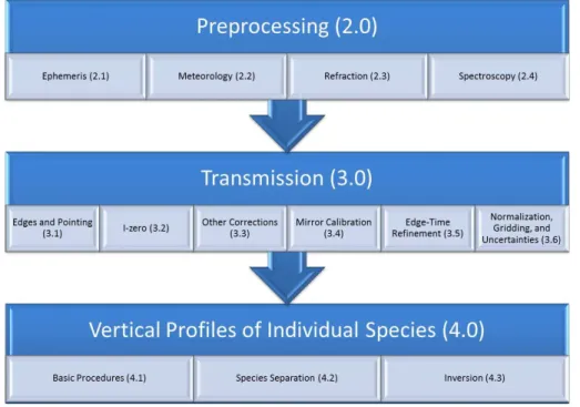
at higher altitudes for certain species due to rapid photochemistry, giving rise to a non-linear variation across the terminator (Chu and Cunnold, 1994), but works well through most of the stratosphere (Cunnold et al., 1989). A general outline of the algorithm can be seen in Fig. 1. The sections that follow provide greater detail on the various steps just outlined and note when and how these differ from the approach of SAGE II version 20
6.2.
2 Preprocessing
Before anything can be done with the solar irradiance data measured by the instrument, a series of preprocessing steps must be performed so that this data can be placed in the proper context. The algorithm needs to determine where the instrument was 25
AMTD
6, 5101–5171, 2013SAGE version 7.0 algorithm: application to SAGE II
R. P. Damadeo et al.
Title Page
Abstract Introduction
Conclusions References
Tables Figures
◭ ◮
◭ ◮
Back Close
Full Screen / Esc
Printer-friendly Version Interactive Discussion
Discussion
P
a
per
|
Di
scussion
P
a
per
|
Discussion
P
a
per
|
Discussi
on
P
a
per
|
meteorological information. In addition, some calculations related to the spectroscopy of the instrument are performed to facilitate later calculations.
2.1 Ephemeris
NASA’s Tracking and Data Relay Satellite System measured the state vectors (posi-tion and velocity) of the ERBS on a regular basis. The Opera(posi-tion Support Computing 5
Division at the Goddard Space Flight Center assimilated this data with an accurate model to determine the spacecraft position and velocity at 60 s intervals, which was provided as level zero ephemeris data to the SAGE processing team. From this orig-inal ephemeris data, events with beta angles greater than 61◦ or events that occur during spacecraft viewed solar eclipses are excluded from further processing. High 10
beta angles (defined as declination of the Sun as measured from the orbital plane) are excluded because the duration of an event (and subsequent ground track) becomes long and the assumption of atmospheric spherical symmetry, used for the inversion process, breaks down. For each remaining event, the original spacecraft state vectors just prior to the start of the event are used as input to the processing algorithm. Using 15
a model for the Earth’s gravitational potential, the equations of motion are calculated and the state vectors are propagated throughout the event. In addition to the state vectors, the position of the Sun is calculated for each time. Then, for each time, co-ordinate and geometrical data required by the algorithm are calculated. This includes information related to the spacecraft (sub-spacecraft latitude, longitude, and altitude), 20
the Sun (angular size, right-ascension, declination, and azimuth), and the tangent point (altitude, latitude, longitude) looking at the center, top, and bottom of the Sun.
The methodologies for these calculations originate from Buglia (1988). For the most part, these methods are straightforward geometry but, in pre-version 7.0 algorithms, some aspects (e.g. sidereal time, precession, nutation, and Sun position) were approx-25
AMTD
6, 5101–5171, 2013SAGE version 7.0 algorithm: application to SAGE II
R. P. Damadeo et al.
Title Page
Abstract Introduction
Conclusions References
Tables Figures
◭ ◮
◭ ◮
Back Close
Full Screen / Esc
Printer-friendly Version Interactive Discussion
Discussion
P
a
per
|
Di
scussion
P
a
per
|
Discussion
P
a
per
|
Discussi
on
P
a
per
|
a change to various numerical constants used in these approximations. However, these changes were not uniformly implemented and data quality in versions prior to version 7.0 was adversely impacted by an inconsistency in ephemeris epoch usage.
In version 7.0, all physical constants (e.g. Earth’s equatorial and polar radii and grav-itational constant) have been updated to those used in the World Geodetic System 5
1984 (WGS84, updated in 2004), which is the current standard. The constants used for the multi-pole expansion of the Earth’s gravitational potential have been updated to those from the Earth Gravity Model 1996 (EGM96) (Lemoine, 1998). In addition, coded routines that relied upon approximations based upon pre-1984 data have been mod-ified to utilize SDP Toolkit routines (Noerdlinger, 1995). Most of these changes result 10
in inconsequential changes to the results with one notable exception. The original rou-tine designed to calculate the position of the Sun suffered from inconsistent ephemeris epoch usage and outdated numerical approximations. The adoption of a Toolkit routine has corrected what was a previously unknown quasi-random error in the altitude reg-istration in the SAGE II data products. For any given event, this correction manifests 15
itself as an altitude offset between SAGE II versions 6.2 and 7.0. This altitude offset can be positive or negative, can have a magnitude up to a few hundred meters, and varies from event to event. While there is no simple dependence upon beta angle or latitude, there is some correlation with time of year, as expected, as shown in Fig. 2.
2.2 Meteorology 20
SAGE processing algorithms require ancillary meteorological data that relates density and temperature to altitude. SAGE II version 6.2 used multiple sources of data to yield density and temperature data (akaP/T data) from the surface up to 100 km. NCEP Reanalysis data (Kalnay et al., 1996) was used first, yieldingP/T data from 1000 mbar up to 10 mbar (∼30 km). Above that, operational model data provided by NCEP was 25
AMTD
6, 5101–5171, 2013SAGE version 7.0 algorithm: application to SAGE II
R. P. Damadeo et al.
Title Page
Abstract Introduction
Conclusions References
Tables Figures
◭ ◮
◭ ◮
Back Close
Full Screen / Esc
Printer-friendly Version Interactive Discussion
Discussion
P
a
per
|
Di
scussion
P
a
per
|
Discussion
P
a
per
|
Discussi
on
P
a
per
|
retrieveP/T data from, namely the 20 km sub-tangent latitude and longitude. The tem-perature and pressure data sets were then combined and interpolated to a standard 0.5 km spaced altitude grid.
Analysis of the version 6.2P/T data revealed a few anomalies where NCEP oper-ational model data are absent, resulting in the use of GRAM-95 data deep into the 5
stratosphere. In addition, an analysis comparing SAGE II and III coincident events re-vealed that SAGE II NCEP operational model temperature data were typically warmer than SAGE III, even though both were using NCEP data sources (Fig. 3). The cause of this bias is unexplained. To maintain as much consistency as possible, a long-term self-consistent meteorological data set was required that spans the lifetimes of all 10
of the SAGE instruments and provides data throughout the stratosphere. The Mod-ern Era-Retrospective Analysis for Research Applications (MERRA) (Rienecker et al., 2011), based on the Goddard Earth Observing System Model (GEOS-5.2) (Rienecker et al., 2008), provides temperature data at 42 pressure levels from the surface up to 0.1 mbar (∼65 km) from 1978 to the present. While this has not yet been implemented 15
in SAGE III, there are plans to use MERRA data for the reprocessing of SAGE III/M3M data to the version 7.0 standard and to use operational GEOS data for the upcoming SAGE III/ISS mission. SAGE II version 7.0 uses MERRA data from the surface up to 0.1 mbar and GRAM-95 above that up to 100 km. Instead of using the actual GRAM-95 temperature values, the GRAM-95 lapse rate is used to extrapolate above the MERRA 20
data. This is done because the MERRA lower mesospheric temperature values are often smaller than those from GRAM-95. Any attempt to merge the two data sets can introduce an artificial inversion layer in the lower mesosphere.
In both versions, afterP/T profiles are determined, number density profiles are cal-culated. In order to have uncertainty estimates in derived quantities in the inversion 25
AMTD
6, 5101–5171, 2013SAGE version 7.0 algorithm: application to SAGE II
R. P. Damadeo et al.
Title Page
Abstract Introduction
Conclusions References
Tables Figures
◭ ◮
◭ ◮
Back Close
Full Screen / Esc
Printer-friendly Version Interactive Discussion
Discussion
P
a
per
|
Di
scussion
P
a
per
|
Discussion
P
a
per
|
Discussi
on
P
a
per
|
values to use at each pressure level (Finger et al., 1993). MERRA also does not pro-vide uncertainty estimates for their model products. We continue to discuss the topic of model uncertainties with the MERRA group. In the meantime, we are currently adapting the NCEP uncertainty values as a rough guideline.
2.3 Refraction 5
Our refraction algorithm calculates the elevation angle (relative to the local horizon-tal plane at the position of the spacecraft) of the refracted Sun (where the instrument sees the Sun) and the total refraction angle of the light ray as a function of wavelength (Fig. 4). It also calculates the layer slant-path matrix with which it determines the to-tal number density of the slant-path air column (mass path) along the curved path of 10
the light ray. These quantities are calculated for each tangent altitude (in 0.5 km incre-ments) from the surface up to 300 km. The methodology remains largely unchanged from version 6.2 and comes from Chu (1983) and Auer and Standish (2000). After re-fraction, tangent point altitudes, latitudes, and longitudes are updated, taking an oblate Earth model into account (Fig. 4).
15
There is one important error in previous versions to note, which is corrected in ver-sion 7.0. As the algorithm determines the refraction angle, it begins at the surface and moves to higher tangent altitudes. At a small threshold value for the refraction angle, this process ceases and remaining refraction angle values are assumed to be zero. However, these values were not explicitly set to zero. The result of this was that if one 20
event hit this threshold at some altitude and the following event hit this threshold value at some lower altitude, then the refraction angle values between these two altitudes would be carried over from the previous event, potentially through multiple events. This generally occurred in the 50–60 km range, and would be interpreted as non-physical characteristics in the atmosphere, which could propagate downward in the inversion 25
AMTD
6, 5101–5171, 2013SAGE version 7.0 algorithm: application to SAGE II
R. P. Damadeo et al.
Title Page
Abstract Introduction
Conclusions References
Tables Figures
◭ ◮
◭ ◮
Back Close
Full Screen / Esc
Printer-friendly Version Interactive Discussion
Discussion
P
a
per
|
Di
scussion
P
a
per
|
Discussion
P
a
per
|
Discussi
on
P
a
per
|
a single event, to zero. As such, correcting this error in version 7.0 did not uncover or correct any biases in prior versions.
2.4 Spectroscopy
The retrieval process requires absorption cross-sections for O3, NO2, the oxygen dimer
(O2-O2), and molecular (Rayleigh) scattering at all wavelengths. This is done by first
5
combining each channel’s measured spectral response function with the solar spec-trum (Kurucz et al., 1984). The spectral response of channels 2, 5, and 6 also incorpo-rate the long-term evolution in the spectral characteristics of their respective band-pass filters. These spectral responses are then combined with cross-section data for each species (i.e. O3, NO2, O2-O2, and Rayleigh) and integrated across each channel’s
10
spectral range. Rayleigh cross-sections (cm2molecule−1) are wavelength-dependent and are calculated in the same fashion as in Bucholtz (1995). O2-O2 cross-sections (cm5molecule−2) are taken to be wavelength-dependent, are assumed to scale with density, and are calculated in the same fashion as Mlawer et al. (1998) (for wave-lengths encompassing channels 1 and 2) and Newnham et al. (1998) (for wavewave-lengths 15
encompassing channels 3 through 7). O3 and NO2 cross-sections (cm2molecule−1) are taken to be both wavelength-dependent and temperature-dependent. In version 6.2, they were derived from the Shettle and Anderson cross-section compilation (Shet-tle and Anderson, 1995), which is the same cross-section compilation that was used in SAGE III version 3.0. In SAGE III version 4.0 (Thomason et al., 2010), however, the O3
20
cross-sections were updated to the Bogumil (SCIAMACHY V3) cross-sections (Bogu-mil, 2003), which had a positive impact on several data products and produced better agreement with in-atmosphere measurements (Pitts et al., 2006). As such, SAGE II version 7.0 uses the SCIAMACHY V3 O3 cross-sections, including companion
mea-surements of NO2 absorption cross-sections encompassing SAGE II measurement 25
AMTD
6, 5101–5171, 2013SAGE version 7.0 algorithm: application to SAGE II
R. P. Damadeo et al.
Title Page
Abstract Introduction
Conclusions References
Tables Figures
◭ ◮
◭ ◮
Back Close
Full Screen / Esc
Printer-friendly Version Interactive Discussion
Discussion
P
a
per
|
Di
scussion
P
a
per
|
Discussion
P
a
per
|
Discussi
on
P
a
per
|
vertical “profiles” of effective cross-sections for these species in each channel, facilitat-ing later computations.
Effective cross-sections are constructed in this fashion because the interactions be-tween species absorption within the band-pass of any channel are negligible. The O3 retrieval is primarily dependent upon observations in channel 3 (600 nm), where the 5
NO2 cross-section has decreased two orders of magnitude from its peak and
con-tributes a negligible amount to the extinction. The NO2retrieval is primarily dependent upon correlative measurements in channels 5 (452 nm) and 6 (448 nm), where the O3
cross-section has decreased nearly two orders of magnitude from the Chappius and displays little to no structure within these narrow band-passes. Aerosol retrievals are 10
primarily dependent upon observations in channel 1, where the cross-sections of both O3and NO2have decreased by several orders of magnitude and contribute a negligible
amount to the extinction.
Due to the nature of the water vapor feature near 940 nm, the use of effective cross-sections is not possible and the absorption must be modeled. Water vapor line data 15
for version 6.2 were provided by Linda Brown (personal communication, 2002), which were later incorporated into the water vapor line data for the 2004 version of HITRAN. The version 7.0 water vapor line data come from the 2008 version of HITRAN (including the 2009 update to water vapor). These line data are used to pre-compute derivatives of absorption as a function of temperature, pressure, and line-of-sight molecular num-20
ber density for later use with an emissivity-curve-of-grown-approximation (EGA) as the forward model for water vapor absorption (Gordley and Russel, 1980).
After SAGE II had been operating for some time, a long-term analysis of the water vapor product showed it to be in poor agreement with other satellites and ground mea-surements. While many possibilities were considered, and eventually ruled out, it was 25
AMTD
6, 5101–5171, 2013SAGE version 7.0 algorithm: application to SAGE II
R. P. Damadeo et al.
Title Page
Abstract Introduction
Conclusions References
Tables Figures
◭ ◮
◭ ◮
Back Close
Full Screen / Esc
Printer-friendly Version Interactive Discussion
Discussion
P
a
per
|
Di
scussion
P
a
per
|
Discussion
P
a
per
|
Discussi
on
P
a
per
|
with the ERBS. An incomplete shut down of the cooling system caused condensation within the instrument. It is believed that the channel filters absorbed water and then subsequently dried out on orbit, affecting their spectral characteristics. Unfortunately, it was impossible to reproduce this in the lab as no original filter material remained and the company that created it was no longer in business. Version 6.2 was the first version 5
to attempt to account for an apparent shift in the location of the water vapor channel filter. In order to attempt to model the filter characteristics, it was decided to adjust the spectral response of the water vapor channel to make the mean SAGE II water vapor data at one latitude and season agree with a HALOE climatological profile for the same latitude and season (northern mid-latitudes in March). The center wavelength and full-10
width at half-max (FWHM) were adjusted and the two data sets were again compared. While it was impossible to completely match these data sets, it was found that the best match came from a center wavelength shift of+10 nm (945 nm) and an increase in the FWHM of 10 % (22 nm). This was then applied to all SAGE II data from 1986 onward. The before and after comparisons of that work can be seen in Fig. 7. (Thomason et al., 15
2004)
With the adoption of the SCIAMACHY V3 ozone cross-section database came a large shift in the Wulf ozone bands that span the SAGE II water vapor channel spec-tral response (Fig. 8). Given the sensitivity of the water vapor retrieval to the details of ozone (Chu et al., 1993), the evolution of the water vapor channel spectral response 20
was reevaluated. A comparison of SAGE II version 6.2 with newer data sets (Fig. 9) shows that, while version 6.2 matches well to HALOE as expected, there is an offset of about 10 % with both SAGE III and Aura MLS, perhaps suggesting the choice of HALOE as a standard for inferring channel drift was not optimal. The channel 2 drift assessment was repeated, except SAGE III water vapor was used to infer the loca-25
AMTD
6, 5101–5171, 2013SAGE version 7.0 algorithm: application to SAGE II
R. P. Damadeo et al.
Title Page
Abstract Introduction
Conclusions References
Tables Figures
◭ ◮
◭ ◮
Back Close
Full Screen / Esc
Printer-friendly Version Interactive Discussion
Discussion
P
a
per
|
Di
scussion
P
a
per
|
Discussion
P
a
per
|
Discussi
on
P
a
per
|
SAGE II is able to measure NO2 by observing the difference in absorption between the two channels located at 452 nm (channel 5) and 448 nm (channel 6). Another look at exoatmospheric data (Fig. 6) shows that, like the water vapor channel, channel 6 may have had a change in spectral response prior to 1990 as a result of the aforementioned thermal vacuum testing incident. We chose a similar, but slightly different approach, to 5
that used to correct the water vapor channel. Since NO2 measurements are derived
primarily from the differential extinction between the two channels, we chose to use one channel to calibrate the other, since the long-term variation in solarI-zero showed channel 5 to be well behaved. The differential effective cross-sections between the two channels were compared to the differences in their exoatmospheric counts. It was as-10
sumed that any difference in the exoatmospheric counts of channel 6 relative to that seen in channel 5 over time were a result of a change in the band-pass of its filter. In this way, a time-dependent fit could be made that allowed the application of a differential cross-section correction to the effective cross-sections in channel 5 to obtain the eff ec-tive cross-sections in channel 6 for any time during the mission. The time-dependent 15
model for the channel 6 spectral band-pass required the determination of the initial properties and the rate of change relative to the observed long-term anomalousI-zero drift. To compute these, the SAGE II NO2stratospheric column abundances were
com-pared to twilight NO2 measurements at Lauder, New Zealand (Johnston and
McKen-zie, 1984). This procedure was applied in version 6.2, though only at one temperature 20
(240 K). The dependence of SAGE II NO2retrieval on O3necessitated a repeat of this
procedure after both the O3and NO2cross-section databases were changed. The
dif-ference in version 7.0 is the implementation of a temperature-dependent differential cross-section correction and the use of SAGE III NO2 data to determine the starting
spectral location of channel 6. The overall quality of SAGE II NO2measurements
rela-25
AMTD
6, 5101–5171, 2013SAGE version 7.0 algorithm: application to SAGE II
R. P. Damadeo et al.
Title Page
Abstract Introduction
Conclusions References
Tables Figures
◭ ◮
◭ ◮
Back Close
Full Screen / Esc
Printer-friendly Version Interactive Discussion
Discussion
P
a
per
|
Di
scussion
P
a
per
|
Discussion
P
a
per
|
Discussi
on
P
a
per
|
3 Transmission
The transmission algorithm combines measured limb-darkening curves with timing and pointing data to produce slant-path optical depths for each tangent altitude between 0.5 km and 100 km in 0.5 km increments. In order to do this, a number of physical and instrumental sources of variation must be compensated for.
5
The series of calculations and corrections were done, in version 6.2, in a mostly linear fashion with some iterative calculation of transmission. It is now recognized that many of these corrections are dependent upon transmission and are thus, in version 7.0, updated throughout these iterations. This section will focus more on the various calculations and corrections that are done and less on the order in which they are 10
computed or how these steps may be iterated.
3.1 Edges and pointing
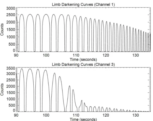
The first step in transmission processing requires that the limb-darkening curves (Fig. 12) be combined with pointing data to place every data packet accurately on the face of the Sun. First the limb-darkening curves in the 1020 nm channel are used 15
to determine where the physical top and bottom edges of the Sun are by looking for the inflection points and the times associated with them. The timing of science packet data and ephemeris pointing data can then be accurately mapped to each other. This is done by assuming that the rate of motion of the scan-mirror is constant during a scan so that each packet of data within a scan can be interpolated to a location on the face 20
of the Sun. This becomes problematic when the bottom of the Sun is obscured by cloud or is below the limb of the Earth, as the calculated inflection point of the limb-darkening curve no longer correlates to the physical edge of the Sun and the calculated scan rate becomes biased high.
The apparent rate of motion of the scan-mirror is a combination of the motion of 25
AMTD
6, 5101–5171, 2013SAGE version 7.0 algorithm: application to SAGE II
R. P. Damadeo et al.
Title Page
Abstract Introduction
Conclusions References
Tables Figures
◭ ◮
◭ ◮
Back Close
Full Screen / Esc
Printer-friendly Version Interactive Discussion
Discussion
P
a
per
|
Di
scussion
P
a
per
|
Discussion
P
a
per
|
Discussi
on
P
a
per
|
a typical event shows that they are generally well behaved and slowly varying with time (Fig. 13a). However, at any time during the event, the attitude actuators on the space-craft (these keep the spacespace-craft in a desired orientation) can turn on or offand cause an abrupt shift in these quantities. The derivatives of these quantities show linearity with respect to time excluding attitude control maneuvers (Fig. 13b). This relationship 5
allows for a linear fit of these quantities to data just above where the rate data be-gins to go bad, which is characterized by large values in the first or second derivatives (Fig. 13c). These fits are then used to reconstruct low altitude rate data (Fig. 13d).
Once the algorithm has good rate data for each scan, the proper tangent altitude and position on the face of the Sun are calculated for each packet. Given the non-10
linearity of the problem of combining refraction effects and an oblate Earth model in determining tangent point altitudes, the algorithm uses an iterative scheme optimized for rapid convergence. During the development of both the SAGE III version 4.0 and SAGE version 7.0 algorithms, the algorithmic uncertainty in determining the tangent point altitude was determined to be better than 20 m. Lower in the atmosphere, where 15
refraction effects can become large, the uncertainty in the tangent point altitude is dominated by uncertainties in the meteorological data. Each packet of data, in each channel, is subsequently assigned a time, tangent altitude, position on the face of the Sun, scan-mirror elevation position, and photodiode count value.
3.2 I-zero 20
In order to create transmission profiles, the algorithm ratios measurements made by the instrument looking at a particular point on the Sun through the atmosphere to the same point seen above the atmosphere. Thus one of the first things the transmis-sion algorithm does is create a standard exoatmospheric limb-darkening curve (I-zero curve) to ratio other scans to. The instrument generally collects between 10 and 20 25
AMTD
6, 5101–5171, 2013SAGE version 7.0 algorithm: application to SAGE II
R. P. Damadeo et al.
Title Page
Abstract Introduction
Conclusions References
Tables Figures
◭ ◮
◭ ◮
Back Close
Full Screen / Esc
Printer-friendly Version Interactive Discussion
Discussion
P
a
per
|
Di
scussion
P
a
per
|
Discussion
P
a
per
|
Discussi
on
P
a
per
|
curve is mapped onto each scan (including the exoatmospheric or I-zero scans), an edge time refinement (see Sect. 3.5) is made for the I-zero scans. A new addition in version 7.0 is the introduction of a time-dependentI-zero correction, which was first introduced in SAGE III version 4.0. A time-dependentI-zero correction benefits high altitude scans by helping to correct for apparent rotation of the scan track across the 5
face of the Sun due to orbital motions (Burton et al., 2010).
Occasionally the instrument would fail to acquire more than one or two exoatmo-spheric scans. This happened sporadically through the lifetime of the instrument, but most notably during the so called “short event” period (from mid-1993 to mid-1994), when a battery problem on the spacecraft reduced the operational scan time of the 10
instrument, causing sunset events to begin later than normal and sunrise events to end earlier than normal. Many of the corrections applied to the data require a minimum number ofI-zero scans (i.e. data over a large range of exoatmospheric altitudes). In prior versions, the absence of this data would often result in anomalous events that were not screened (i.e. dropped) by the algorithm and required the user to manually 15
screen them out (Wang et al., 2002). In version 7.0, all events without a minimum number ofI-zero scans are dropped from processing and flagged accordingly.
3.3 Other corrections
Once anI-zero curve is established (and mapped to each scan), a preliminary trans-mission can be computed for each scan. This then allows the calculation of a few 20
corrections that need to be made. An initial correction for Rayleigh attenuation is done (for the benefit of other corrections) and a polar mesospheric cloud (PMC) detection routine is run (Burton and Thomason, 2000). While no overall correction is made in the presence of PMCs, the use of data within PMCs will be avoided when determining the mirror calibration (see Sect. 3.4). A sunspot detection routine is also run and measure-25
AMTD
6, 5101–5171, 2013SAGE version 7.0 algorithm: application to SAGE II
R. P. Damadeo et al.
Title Page
Abstract Introduction
Conclusions References
Tables Figures
◭ ◮
◭ ◮
Back Close
Full Screen / Esc
Printer-friendly Version Interactive Discussion
Discussion
P
a
per
|
Di
scussion
P
a
per
|
Discussion
P
a
per
|
Discussi
on
P
a
per
|
filtering (i.e. it would often omit all data from the start of a sunspot to the edge of the Sun) and a more robust algorithm has been introduced for version 7.0.
As the SAGE II instrument began taking data during each event, a small transient was observed in channels 5 and 6. This so-called thermal shock needed to be ac-counted for in the data processing. For sunset events, this is relatively easy as the 5
data are fairly homogenous (exoatmospheric scans) and any time dependency is eas-ily recognized and removed. For sunrise events, however, the transient occurs while the instrument is looking through the attenuated atmosphere and the correction is nec-essarily at low altitudes. In this case, scan-to-scan variations in the channel 5 and 6 differential extinction at a given altitude, which are correlated in time across multiple 10
scans, are examined. By looking at the ratio of channel 6 to channel 5, which is used for the NO2 retrieval, the algorithm determines the rate of change of differential
ex-tinction, which is then integrated to produce a correction that is applied to these two channels. The impact on the transmission in these channels is on the order of 0.25 %, whereas the impact on other channels (were it to be applied) would be no more than 15
0.05 % (SPARC/IOC/GAW, 1998).
3.4 Mirror calibration
SAGE operates by using a scan-mirror to move the instrument field-of-view up and down across the solar disk (normal to the Earth’s limb). The reflectivity of the scan-mirror varies slightly with the angle of incidence and requires calibration. This is not 20
an absolute reflectance calibration, as only the relative change in reflectivity with an-gle is required. In version 6.2, this calibration was determined through a quadratic fit to high altitude transmission data as a function of altitude and performed only once at the end of transmission processing. In version 7.0, this quadratic fit is to high alti-tude transmission data as a function of the elevation angle of the scan-mirror and is 25
AMTD
6, 5101–5171, 2013SAGE version 7.0 algorithm: application to SAGE II
R. P. Damadeo et al.
Title Page
Abstract Introduction
Conclusions References
Tables Figures
◭ ◮
◭ ◮
Back Close
Full Screen / Esc
Printer-friendly Version Interactive Discussion
Discussion
P
a
per
|
Di
scussion
P
a
per
|
Discussion
P
a
per
|
Discussi
on
P
a
per
|
(higher altitudes) are used for the fit, an extrapolation of the correction term to larger angles (lower altitudes) is necessary to correct attenuated data. An example of the mir-ror correction can be seen in Fig. 14, demonstrating that the angular dependence of the reflectivity of the scan-mirror is on the order of 0.5 %.
3.5 Edge-time refinement 5
The edge-time refinement algorithm is designed to minimize any biases in the limb-darkening curves created by slight errors of the initial calculation of the edge times of each scan. The measured solar intensity of a scan (I) in a given channel (λ) is a function of both position on the face of the Sun (p) and altitude (z), which are themselves both functions of time (t), and can be written as
10
I(λ,p(t),z(t))=I0(λ,p(t))T(λ,z(t))+ε(λ) (1)
whereI0 is theI-zero limb-darkening curve,T is the slant-path transmission, and εis
the error in the measurements or estimates. Since there is some inherent uncertainty in the calculated edge times, Eq. (1) can realistically be rewritten as
I(λ,p(t+ε
t),z(t+εt))=I0(λ,p(t))T(λ,z(t))+ε(λ) (2)
15
whereεtis related to uncertainties in the edge times. There are two cases that can be
considered separately. The first case is for high altitude measurements whereT(z)=1, and Eq. (2) can be expanded into
I(λ,p(t+ε
t))=I(λ,p+εp)=I0(λ,p)+
dI0(λ,p)
dp εp=I0(λ,p)+
dI0(λ,p)
dp (c1+c2p) (3)
where I0 is the estimate for the I-zero curve and c1 and c2 are the linear shift and
20
AMTD
6, 5101–5171, 2013SAGE version 7.0 algorithm: application to SAGE II
R. P. Damadeo et al.
Title Page
Abstract Introduction
Conclusions References
Tables Figures
◭ ◮
◭ ◮
Back Close
Full Screen / Esc
Printer-friendly Version Interactive Discussion
Discussion
P
a
per
|
Di
scussion
P
a
per
|
Discussion
P
a
per
|
Discussi
on
P
a
per
|
finite differences and a multiple linear regression technique is used to obtain the shift and stretch terms, which yield the correction to the edge times.
The second case involves measurements in the atmosphere where T(z) can no longer be ignored. In this case, Eq. (2) can be expanded into
I(λ,p(t+ε
t),z(t+εt))=I0(λ,p(t))T(λ,z(t))+
d
dt(I0(λ,p(t))T(λ,z(t)))εt (4)
5
I(λ,p(t+ε
t),z(t+εt))=I0T+
I0
dT
dz
dz
dt +T
dI0
dp
dp
dt
(c1+c2t) (5)
wherec1 andc2are again the linear shift and stretch coefficients. Following the same
procedure, the correction to the edge times is obtained. Since the pair of edge times apply equally to all spectral channels, the derivatives are performed at each wavelength 10
and used together in the regression calculation. The shift and stretch algorithm has the effect of removing spectrally and vertically correlated noise in the transmission profile, typically at low altitudes (Fig. 15).
3.6 Normalization, gridding, and uncertainties
In order to calculate the various corrections already outlined, the algorithm iteratively 15
computes transmission values for each packet. In order to mitigate effects remaining from residual edge time uncertainties, the outer 10 % of the solar disk is omitted. After the algorithm has undergone several iterations of calculating transmission and applying corrections, it computes the final transmission profile. A running median filter is applied through altitude sorted transmission packets to minimize the impact of strong outliers, 20
and then smoothed with a boxcar average. The filtering process is performed in altitude and the filtering/smoothing parameters correspond to 1.0 km so that all transmission data meet the Nyquist sampling criteria for a 0.5 km gridded profile. An example of an intermediate transmission profile and a final transmission profile is shown in Fig. 16. The transmission data are then interpolated to the 0.5 km grid, and the variance of the 25
AMTD
6, 5101–5171, 2013SAGE version 7.0 algorithm: application to SAGE II
R. P. Damadeo et al.
Title Page
Abstract Introduction
Conclusions References
Tables Figures
◭ ◮
◭ ◮
Back Close
Full Screen / Esc
Printer-friendly Version Interactive Discussion
Discussion
P
a
per
|
Di
scussion
P
a
per
|
Discussion
P
a
per
|
Discussi
on
P
a
per
|
In version 6.2, the statistics of this fit were used for the uncertainty in the transmis-sion value in each bin. In vertransmis-sion 7.0, we have incorporated an additional uncertainty term, namely a calculated uncertainty in the original I-zero curve, meant to account for variations between the exoatmospheric scans used to create theI-zero curve and the resultingI-zero curve itself. These minor variations between each exoatmospheric 5
scan are highly correlated with position on the solar disk, but have no discernible time-dependency (i.e. they are not detected and filtered by the time-dependentI-zero cor-rection). It is believed that these variations represent physical features in the Sun’s pho-tosphere (e.g. granulation) combined with the apparent rotation of the solar disk during the event, as opposed to instrumental noise. These variations manifest themselves as 10
low amplitude oscillatory patterns in high altitude transmission (on the order of 0.1 %) that are periodic in altitude (due to their high correlation with surface features on the Sun) and correlated between channels (Fig. 17). An extension of the time-dependent
I-zero algorithm to compensate for this effect is in development. Lastly, all slant-path transmission profiles are converted to slant-path optical depth profiles.
15
4 Vertical profiles of individual species
The inversion algorithm takes slant-path optical depth profiles and, along with other data such asP/T data, separates them into species specific slant-path optical depth profiles before finally inverting them into vertical profiles of O3 and NO2 number den-sities, H2O volume mixing ratio, and aerosol extinction. While much of this follows the
20
AMTD
6, 5101–5171, 2013SAGE version 7.0 algorithm: application to SAGE II
R. P. Damadeo et al.
Title Page
Abstract Introduction
Conclusions References
Tables Figures
◭ ◮
◭ ◮
Back Close
Full Screen / Esc
Printer-friendly Version Interactive Discussion
Discussion
P
a
per
|
Di
scussion
P
a
per
|
Discussion
P
a
per
|
Discussi
on
P
a
per
|
4.1 Basic procedures
The viewing geometry of SAGE is such that at each tangent height the instrument looks through the atmosphere, it is also looking through a slant-path column of air that incorporates all of the tangent heights above it. Accounting for refraction, a triangular path-length matrix is computed. The slant-path total column at each tangent height, 5
derived from a matrix multiplication of the path-length matrix and density profile, is thus comprised of the sum of partial slant-path columns from all overlying 0.5 km thick lay-ers. This simple matrix operation allows for an “onion peeling” process to be performed later for inverting a species’ slant-path optical depth profile to the species density pro-file.
10
The first step in the retrieval of vertical profiles of individual species is to ac-count for and remove the contributions of molecular (Rayleigh) scattering in all channels and O2-O2 absorption in a subset of channels. O2-O2 cross-sections (cm5molecule−1) are scaled with density and both O2-O2and Rayleigh effective cross-sections (cm2molecule−1) are combined with the slant-path total column to convert to 15
slant-path optical depths, which are then subtracted from each channel.
4.2 Species separation
The species separation in SAGE II is performed using five of the seven channels si-multaneously (1020, 600, 525, 452, and 448 nm) and is separated into three altitude regions: altitudes where some of the 5 channels are no longer available, altitudes in 20
which all five channels are available, and altitudes above which it is believed there is no aerosol extinction. These five channels are used because the poor quality of the 386 nm channel prevents its use in the broad retrieval. Significant absorption by water vapor occurs only in the 940 nm channel and is inverted in a separate process.
The first step is to find the highest extent to which one of the five channels is not 25
AMTD
6, 5101–5171, 2013SAGE version 7.0 algorithm: application to SAGE II
R. P. Damadeo et al.
Title Page
Abstract Introduction
Conclusions References
Tables Figures
◭ ◮
◭ ◮
Back Close
Full Screen / Esc
Printer-friendly Version Interactive Discussion
Discussion
P
a
per
|
Di
scussion
P
a
per
|
Discussion
P
a
per
|
Discussi
on
P
a
per
|
NO2, and aerosol, though at longer wavelengths (particularly 1020 nm) the contribution from gas species absorption becomes vanishingly small. At this point we have mea-surements with seven unknowns: O3, NO2, and aerosol at each wavelength. We solve
this set of equations using a least-squares solution where we approximate the aerosol contribution at 600 and 448 nm as the linear combination of aerosol at 1020, 525, and 5
452 nm. The full set of species separation equations to be solved can be expressed as
c1(λi)ODAer(λ1)+
σO3(λi) σO3(λ3)
ODO3(λ3)+c2(λi)ODAer(λ4)+c3(λi)ODAer(λ5)
+σNO2(λi)
σNO2(λ5)
ODNO2(λ5)=OD(λi)
wherei={1, 3, 4, 5, 6}is the channel number,σ(λ
i) is the effective cross-section of the
10
stated species at the given channel, OD(λi) is the slant-path optical depth of the stated
channel, and the channel specific aerosol, O3, and NO2 ODs are the unknowns. The
coefficients for this process (c1,c2, andc3) are determined using an ensemble of single mode log-normal size distributions of sulfate aerosol at stratospheric temperatures, though, in practice, composition is of secondary importance. The ensemble of log-15
normal size distributions spans the observed wavelength-dependence of the aerosol spectra.
Once O3 and NO2 ODs are determined, their relative contributions in the 940 and
386 nm channels can be removed and aerosol OD in the 386 nm channel is retrieved as a residual. Aerosol OD in the water vapor channel is calculated from the 525 and 20
1020 nm aerosol values, using separate weighting coefficients determined from the use of the 525 to 1020 aerosol OD ratio. Once the aerosol contribution in the water vapor channel is determined, the actual water vapor OD is calculated as a residual. This process separates the various species from lower altitudes (typically in the middle to upper troposphere) up to some maximum altitude (typically set to 75 km).
25
AMTD
6, 5101–5171, 2013SAGE version 7.0 algorithm: application to SAGE II
R. P. Damadeo et al.
Title Page
Abstract Introduction
Conclusions References
Tables Figures
◭ ◮
◭ ◮
Back Close
Full Screen / Esc
Printer-friendly Version Interactive Discussion
Discussion
P
a
per
|
Di
scussion
P
a
per
|
Discussion
P
a
per
|
Discussi
on
P
a
per
|
becomes the dominant signal. This noise is a carryover of the channel-correlated solar structure noise first discussed in Sect. 3.6, which does not dampen at higher altitudes. Much of this noise ends up being interpreted by the algorithm as aerosol and detri-mentally affects the simultaneous retrieval of all species. To compensate for this in version 6.2, a separate retrieval scheme was used that uses only 4 channels (600, 5
525, 452, and 448 nm) and assumes that no aerosol is present to calculate O3 OD in
the 600 nm channel and NO2OD in the 448 nm channel. Water vapor was again treated as a residual in the 940 nm channel. In lieu of more adaptive methods, this process be-gan at 40 km up to some maximum altitude (typically 75 km). Thereafter, the 5-channel retrieval was transitioned into the “no aerosol” retrieval between 40 and 45 km. The 10
version 7.0 algorithm utilizes the data to determine how to transition into regions where the inclusion of aerosol in the retrieval is no longer necessary, the methods of which are outlined later in this section.
For altitudes below the 5-channel retrieval, there is no longer valid data in the 448 nm channel and thus NO2 cannot be retrieved. Instead, the NO2 OD profile from the
5-15
channel retrieval is inverted to get extinction values and the algorithm reconstructs ODs at lower altitudes by assuming the NO2mixing ratio is zero. The OD contribution from NO2at lower altitudes is then removed from all channels. With NO2removed, the
algorithm begins working from the bottom of the 5-channel retrieval and moves down. It first uses a 4-channel retrieval (1020, 600, 525, and 452 nm) so long as there is valid 20
data and then transitions to a 3-channel retrieval (1020, 600, and 525 nm) when nec-essary. The main retrieval algorithm stops if there is no longer any valid data in any of these three channels. Aerosol extinction in the 1020 nm channel is thereafter retrieved as low as data exists. These data are then used to estimate the contribution of aerosol in the 940 nm channel so that water vapor can again be calculated as a residual. 25
AMTD
6, 5101–5171, 2013SAGE version 7.0 algorithm: application to SAGE II
R. P. Damadeo et al.
Title Page
Abstract Introduction
Conclusions References
Tables Figures
◭ ◮
◭ ◮
Back Close
Full Screen / Esc
Printer-friendly Version Interactive Discussion
Discussion
P
a
per
|
Di
scussion
P
a
per
|
Discussion
P
a
per
|
Discussi
on
P
a
per
|
for values around the observed value. This accounts for a small degree of non-linearity observed in the fits to 600 and 448 nm aerosol extinction. In reality, this is a distinctly second order correction but seems to reduce the sensitivity of the quality of the ozone data product to aerosol, particularly when aerosol levels are high. However, for the same reasons that version 6.2 has a “no aerosol” retrieval, at altitudes near and above 5
40 km, the 525 to 1020 aerosol OD ratio can begin to vary wildly through non-physical numbers. This has a detrimental effect on the second iteration retrievals, producing extremely “noisy” data above 35 km. In version 7.0, once the retrieved aerosol OD in each channel drops below a pre-determined threshold, a non-linear least squares fit is made to the data in the form of an exponential decay curve. Above the altitude where 10
these fits drop below the amplitude of the noise, the fits are used for the 525 to 1020 ratio instead of the actual data. The second iteration retrievals then have far more realistic weighting coefficients to work from.
While the use of fits to determine the 525 to 1020 ratio does improve the quality of the 5-channel retrievals, particularly above 35 km, it can still suffer from the same lim-15
itations that necessitated the use of a “no aerosol” retrieval above 40 km, namely the fact that the aerosol ODs at higher altitudes can still become non-physical and detri-mentally affect the simultaneous retrieval of all species. Typically this is a byproduct of retrieved non-physical aerosol OD values in the shorter wavelengths at higher altitudes detrimentally impacting the retrieved values in longer wavelengths. This had the ten-20
dency (in version 6.2) to result in O3and NO2values that were biased high at altitudes
above∼40 km. To compensate for this, in version 7.00, the algorithm looks only at the 600 nm channel to retrieve ozone in these altitude regimes. When the fit to the 600 nm aerosol OD drops below a certain threshold, the algorithm subtracts out the fit (which is generally below the “noise level”) and inverts only the remaining 600 nm OD to re-25
trieve ozone. A more adaptive algorithm is being developed for retrieving NO2at higher altitudes though, for now, the high bias persists from version 6.2.
AMTD
6, 5101–5171, 2013SAGE version 7.0 algorithm: application to SAGE II
R. P. Damadeo et al.
Title Page
Abstract Introduction
Conclusions References
Tables Figures
◭ ◮
◭ ◮
Back Close
Full Screen / Esc
Printer-friendly Version Interactive Discussion
Discussion
P
a
per
|
Di
scussion
P
a
per
|
Discussion
P
a
per
|
Discussi
on
P
a
per
|
or 1020 aerosol contribution became negative, the algorithm assumed there was no longer any aerosol contribution above that altitude in the water vapor channel (mainly because the weighting coefficients could not be determined from a negative ratio). However, it is possible, due to noise, for the aerosol contribution to become negative but then become some non-negligible positive number again. This should have manifested 5
itself as noise in the data, but was instead being artificially removed. By using the fits to the aerosols to determine the 525 to 1020 ratio, weighting coefficients could be applied to the real data (be it positive or negative) through the entire retrieval range. This has benefited the retrieval greatly as, after the removal of O3and NO2, the aerosol contribution to the water vapor channel can still be a significant fraction of the remaining 10
signal in some cases.
4.3 Inversion
After species separation, water vapor is the first retrieved species. The slant-path op-tical depth data are first converted to extinction and then smoothed to help mitigate noise in the weak signal. The algorithm to retrieve water vapor mixing ratio remains 15
mostly unchanged from Chu et al. (1993) with one small exception. Originally the pro-cess began at 50 km and worked down. The algorithm requires a small range of altitude at the top of the retrieval process to establish the abundance and scale height of the H2O profile as a boundary condition. Improvements in the version 7.0 transmission allow the starting altitude to be moved up to 60 km. This, combined with the aforemen-20
tioned aerosol fit method, has greatly improved the water vapor product above 40 km. In version 6.2, water vapor mixing ratio profiles would suffer from a characteristic “hook” towards unrealistically large values nearing 50 km. This can also be seen in SAGE III version 4.0 water vapor mixing ratio profiles. With these modifications to the retrieval, this “hook” has been removed (Fig. 18).
25
AMTD
6, 5101–5171, 2013SAGE version 7.0 algorithm: application to SAGE II
R. P. Damadeo et al.
Title Page
Abstract Introduction
Conclusions References
Tables Figures
◭ ◮
◭ ◮
Back Close
Full Screen / Esc
Printer-friendly Version Interactive Discussion
Discussion
P
a
per
|
Di
scussion
P
a
per
|
Discussion
P
a
per
|
Discussi
on
P
a
per
|
the hygropause, SAGE II ozone retrievals have consistently been biased low when compared with other data (Wang et al., 2002). This feature was turned offin SAGE III version 4.0, due to uncertainty of the quality of the relative spectroscopy used between the water vapor channel and the 600 nm channel, with beneficial results (Wang et al., 2006). For the same reason, this feature has also been turned offin SAGE II version 5
7.0. It is important to note, however, that this has not completely corrected the low bias in SAGE II tropospheric ozone data.
Once the algorithm has run through both iterations, it has produced vertical water vapor volume mixing ratio and NO2 number density profiles. All that remains is to
in-vert the O3 and various aerosol slant-path column optical depth profiles into vertical 10
extinction profiles. As with NO2, the O3 vertical extinction profile is then converted to a vertical number density profile by simply dividing by the effective cross-section. The inversion technique used in version 7.0 is different from that used in version 6.2, which utilized Twomey’s modification of Chahine’s algorithm (Chahine, 1972; Twomey, 1975) to retrieve extinction values and a simple onion-peeling technique to retrieve uncer-15
tainty estimates. Twomey–Chahine was found to have several undesirable behaviors. It would not allow negative values and therefore introduced a positive bias in regions of the density (extinction) profile where the signal to noise ratio was small, typically at the higher altitude end of the retrieved profile. It also systematically approached the solu-tion from one direcsolu-tion and stopped once the tolerance criterion was met, producing 20
another form of bias as a result. Lastly, its use introduced discontinuities in the profile when the slant-path extinction fell below a preset value and vertical smoothing was activated. Given the high quality of the SAGE II version 7.0 transmission profiles and the algorithmic limitations of the Twomey–Chahine inversion method, it was replaced entirely with onion-peeling in version 7.0.
25
AMTD
6, 5101–5171, 2013SAGE version 7.0 algorithm: application to SAGE II
R. P. Damadeo et al.
Title Page
Abstract Introduction
Conclusions References
Tables Figures
◭ ◮
◭ ◮
Back Close
Full Screen / Esc
Printer-friendly Version Interactive Discussion
Discussion
P
a
per
|
Di
scussion
P
a
per
|
Discussion
P
a
per
|
Discussi
on
P
a
per
|
5 Results of version 7.0
This paper describes the SAGE II version 6.2 and version 7.0 algorithms. Prior ver-sions of SAGE II data products have been well validated (e.g. Wang et al., 2002) and included in numerous international assessments (e.g. WMO, 2011). Several of the ver-sion 7.0 changes affect the quality of these data products and a brief assessment of 5
the differences seen in the version 7.0 data products follows.
5.1 Event comparisons
Figure 19 shows several comparison plots of ozone. The changes in ozone from ver-sion 6.2 to verver-sion 7.0 come almost entirely from the change in spectroscopy, resulting in a nearly uniform decrease in concentration of∼1.5 % in the stratosphere. The mag-10
nitude of the offset increases to about 2 % above 40 km due to the removal of the “no aerosol” method of retrieval. The large increase in ozone below 10 km is a result of the removal of the water vapor correction to ozone. The difference between the mean and median below 20 km is a result of using onion-peeling for inversion instead of Twomey– Chahine, as the outliers in version 6.2 were biased positive whereas in version 7.0 they 15
can take on negative values; though overall the same number of outliers exist. While the changes move SAGE II ozone values further from SAGE III concentrations by about 1.5 % despite using the same spectroscopy, the changes in the retrieval method make the altitude dependency of the offset more consistent.
Given the diurnal nature of NO2, sunrise and sunset events are compared sepa-20
rately. Figure 20a and b shows comparison plots for sunset and sunrise NO2,
respec-tively. Due to changes in spectroscopy, the overall concentration of sunset NO2 has
dropped by 5–10 % in the mid-stratosphere. The large decrease below 20 km is again a result of using onion-peeling instead of Twomey–Chahine for inversion. As previously mentioned, sunset NO2values are biased high above 40 km and an algorithm to better
25