Guidelines for the Fitting of Anomalous
Diffusion Mean Square Displacement Graphs
from Single Particle Tracking Experiments
Eldad Kepten1*, Aleksander Weron2, Grzegorz Sikora2, Krzysztof Burnecki2, Yuval Garini1
1Physics Department & Institute of Nanotechnology, Bar Ilan University, Ramat Gan, Israel,2Hugo Steinhaus Center, Institute of Mathematics and Computer Science, Wroclaw University of Technology, Wroclaw, Poland
Abstract
Single particle tracking is an essential tool in the study of complex systems and biophysics and it is commonly analyzed by the time-averaged mean square displacement (MSD) of the diffusive trajectories. However, past work has shown that MSDs are susceptible to signifi-cant errors and biases, preventing the comparison and assessment of experimental stud-ies. Here, we attempt to extract practical guidelines for the estimation of anomalous time averaged MSDs through the simulation of multiple scenarios with fractional Brownian mo-tion as a representative of a large class of fracmo-tional ergodic processes. We extract the pre-cision and accuracy of the fitted MSD for various anomalous exponents and measurement errors with respect to measurement length and maximum time lags. Based on the calculat-ed precision maps, we present guidelines to improve accuracy in single particle studies. Im-portantly, we find that in some experimental conditions, the time averaged MSD should not be used as an estimator.
Introduction
The analysis of single particle trajectories has become a standard procedure in the analysis of experimental and theoretical systems [1–7]. In biological systems, that are intrinsically stochas-tic in nature, single parstochas-ticles have been measured in all cellular environments and stages, both in vivo and in vitro [8–17].
Since cellular environments are complex microscopic systems with a strong thermal compo-nent [17], the motion of single particles, even if directed, incorporates a random diffusive com-ponent, which must be characterized in order to build a physical picture of the system [18–24]. A common tool by which the diffusion of a single particle is classified is the time averaged mean square displacement (TAMSD) [14–17,25–31]:
d2 ðtÞ ¼
PL=d n
m¼1 ðxðmdþtÞ xðmdÞÞ 2
L=d n ; ð1Þ
OPEN ACCESS
Citation:Kepten E, Weron A, Sikora G, Burnecki K, Garini Y (2015) Guidelines for the Fitting of Anomalous Diffusion Mean Square Displacement Graphs from Single Particle Tracking Experiments. PLoS ONE 10(2): e0117722. doi:10.1371/journal. pone.0117722
Academic Editor:Yaakov Koby Levy, Weizmann Institute of Science, ISRAEL
Received:November 2, 2014
Accepted:December 30, 2014
Published:February 13, 2015
Copyright:© 2015 Kepten et al. This is an open access article distributed under the terms of the
Creative Commons Attribution License, which permits unrestricted use, distribution, and reproduction in any medium, provided the original author and source are credited.
Data Availability Statement:All relevant data are within the paper.
defined here for a trajectoryx(t) of lengthL, taken at sampling time-intervalsδand the
averag-ing window isτ=nδ. For normal diffusion (not necessarily Brownian or Gaussian [32]) the
MSD is linear in timed2
ðtÞ ¼D1t, whereD1is the generalized diffusion coefficient which in-cludes all constant prefactors, depending on the diffusion mechanism.
The TAMSD may be of any functional form, but in many cases it is a power law function
over long times,d2
ðtÞ ¼D
at a
[33,34]. The anomalous exponentαis related to fundamental
characteristics of the stochastic process, such as temporal correlations and the distribution of particle steps and it is necessary for predicting the future particle motion, first passage times and more [35].
There are various classes of anomalous diffusion and they all result from the breaking of the assumptions behind normal Brownian diffusion, see [36] for a recent review. Continuous time random walks (CTRW) which have long tailed jump distributions or waiting times between jumps exhibit weak ergodicity breaking of a normal TAMSD. Variation in the surrounding space may lead, among other models, to heterogeneous diffusion processes (HDP) and ob-structed diffusion, both with unique characteristics. If the stochastic process is not Markovian and there is a temporal correlation between steps, another class of anomalous diffusion is exhibited. Fractional Brownian motion (FBM) for example has self-similar Gaussian steps with a correlation that decays as a power law. A general description of processes with temporal step correlations can be obtained through the ARFIMA framework that generalizes fractional dynamics through a discrete generating process [37].
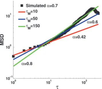
The TAMSD is normally fitted through the logarithm ofeqn. 1as a function ofτup to a
maximalτ
M,Fig. 1:
logðd2ðtÞÞ ¼logðDaÞ þalogðtÞ; t¼1;. . .;t
M: ð2Þ
Fig 1. Fitting a time averaged MSD with various maximum time lags.A trajectory withα= 0.7,L= 29,σ=
0.5 was simulated (black squares) and fitted for variousτ
Mvalues. While the smallτMfitting (redτM= 10 and
blueτ
M= 50) underestimatedα, the largeτM(greenτM= 150) gives an overestimation. Clearly, selecting the
optimalτMvalue is not trivial as both small and large values may lead to erroneous results. Graphically
assessing the quality of the fit does not help select the bestτ
Meither.
doi:10.1371/journal.pone.0117722.g001
Several studies have shown that the TAMSD is a problematic estimator [25,38,39]. The in-ternal correlations between the averaged quantities merit the central limit theorem inapplicable and large variations are introduced with increasingτ. In addition, measurement errors lead to
short time artifacts in the estimated TAMSD. For example, when a normally distributed mea-surement error (with varianceσ2and zero mean) is introduced to ergodic anomalous diffusion
measurements, the theoretical TAMSD is [40,41]
d2
ðtÞ ¼Data
þ2s2
ð3Þ
For a discussion of the influence of various error mechanisms on the TAMSD of CTRW dif-fusion, see [42].
For normal diffusion various alternative and complementary techniques have been devel-oped [39,43] that overcome these problems. In addition, anomalous diffusion can be efficiently estimated when an ensemble of trajectories is available [41]. However, when analyzing single trajectories of particles that exhibit anomalous diffusion, these techniques are inadequate and one is left with the direct estimation of the functional form of the TAMSD.
When analyzing experimental data, one has a limited trajectory length and for single particle trajectories, it is often shorter than 103time points. This raises another fundamental problem in implementation ofeqn. 2. Since the variance of the TAMSD increases withτ, taking largeτ
M
re-duces the accuracy of the estimation. However, since the data is limited, the MSD also fluctuates at smallτvalues. In addition, as seen above, measurement errors introduce an offset at smallτ’s.
Thus one must find an optimalτMthat balances between the need to fit severalτ’s ineqn. 2
while avoiding the fluctuating nature of the TAMSD at large times. We stress that simply taking very small or largeτMvalues does not improve the estimation ofα, as can be seen inFig. 1.
To the best of our knowledge, there is no systematic study of the optimalτ
Mvalue for the
es-timation of the anomalous exponent in the presence of measurement errors. As a result, there are no standards or guidelines for fitting the TAMSD, which introduces difficulty in assessing the accuracy and precision of extracted values and comparison between studies. Furthermore, we show that the data analysis can be optimized by realizing the specific experimental conditions.
In what follows we study the performance of the TAMSD as an estimator for the anomalous exponent, depending on trajectory length, measurement error and the true anomalous expo-nent. This is done through the simulation of thousands of trajectories and fitting their individ-ual TAMSDs. We study FBM diffusion, which we chose as an experimentally observed motion and a representative of the common class of ergodic anomalous diffusion [24]. We calculate the accuracy and precision of the TAMSD estimator as a function of the maximal fitted time lag,τ
M, for different combinations of the diffusion parameters. The results allows us to identify
an optimal M in each case and by taking all the extracted information together, we identify sev-eral guidelines, or best practices, for fitting of anomalous TAMSDs. We find that even a rough estimation of the measurement error and the expected regime of the anomalous exponent can greatly improve the accuracy of the extracted parameters.
Our approach can be applied to any process with a definedαthat one can simulate in order
to find the best estimation conditions, even ifDαvaries between trajectories such as in CTRW
or HDP. Although we focus on the more difficult experimental case of short trajectories, our general guidelines apply also for longer trajectories.
Methods
Trajectories {xi(t)} were simulated using the MATLABwfbmfunction [44] which is a common
as proposed in [45]. In addition, we normalized the standard deviation of the increments for each trajectory to one, so thatDα= 1. Notice that FBM has stationary Gaussian increments, so
normalizing the standard deviation uniquely defines the stochastic process for a givenα.
A series of independent normally distributed measurement errors {ε
i(t)} with zero mean
and standard deviationσwas added to each trajectory. Since all trajectories were normalized,
the relative magnitude of the measurement error compared to {xi(t)} is set only byσ. Also, note
that for any uncorrelated measurement noise distribution that has a defined second moment, the magnitude ofσis enough to characterize its effect on the TAMSD.
We look into four representative cases of anomalous diffusion:strong subdiffusionα= 0.3,
weak subdiffusionα= 0.7,weak superdiffusionα= 1.3 andstrong superdiffusionα= 1.7. In
each case, three error regimes are studied: lowσ= 0.1, mediumσ= 0.5 and strongσ= 1.
For each pair ofαandσwe study trajectories of lengthL= 10 to 2000. For each trajectory
we fit the TAMSD according toeqn. 2for all possibleτMup toL/2. We then repeat the
calcula-tion of the TAMSD and its fitting for 1000 trajectories for eachLandτ
M. Thus for each (α,σ)
pair we have a set ofαi(L,τM) withi= 1,. . ., 1000 for every (L,τM) combination.
We are now faced with the problem of identifying what is a‘good’fitting regime. One ap-proach is to characterize the distribution ofP(αi) for each (L,τM) pair in each (α,σ) mapping.
Then, one can estimate the probability of the fitted value to fall in a certain range around the true anomalous exponent. However, this approach is problematic asP(αi) is not necessarily
normal. In fact, past studies have shown that the distribution ofhδ2(τ)iis highly non Gaussian
[46,47], leading to similar expectation forP(αi). As a result, analytically estimating
probabili-ties will demand the characterization of general distributions.
Thus we take a different, more applicable approach where for each (L,τM), we extract the
fractionF(α,σ)(L,τM) ofαithat are in the range [α−0.1,α+ 0.1]. We chose these limits since
they provide reasonable accuracy in biophysical studies while maintaining reasonableFvalues for different (α,σ) maps.Fis an intuitive parameter for the precision of the fitting, as higher
values mean more precise fitting.
In some cases, one can extract multiple trajectories of the same stochastic process. This is for example the case in various simulation studies. Thus by averaging over fitted single particleα
i’s, one may hope to converge withhαiitoα. We define the bias asB(α,σ)(L,τM) =
hαii(L,τ
M)−α. This bias is a measure of the accuracy of the MSD estimator.
Results
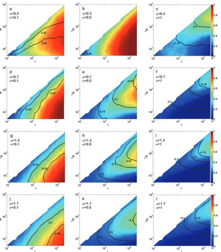
Fig. 2shows a heat map ofFwith contour lines of the biasBfor each measurement lengthL andτM. As observed, it is easy to find the optimalτMfor fitting, i.e. optimalFandBconditions.
For example, for a thousand time point trajectory in the weakly subdiffusive regime (α= 0.7)
withσ= 0.5, we find a maximalF0.63 forτM= 50. In addition, 0<B<−0.1 gives
reason-able results for averaged TAMSDs. However, if the trajectory is only 100 time points long, it is best to useτM= 10, givingF0.36 and−0.1<B<−0.2.
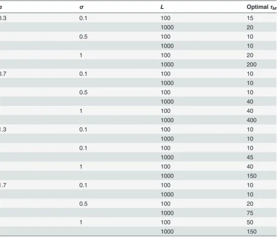
We recommend the extraction of the optimalτMfor each experiment depending on the
exact conditions.Table 1, however, gives a quick look-up table for optimalτMforL= 100 and
1000 depending onαandσand can be used to quickly analyze experimental data.
We now describe several trends in the maps ofFandB. The two fundamental observations are that lowerαorσusually give better estimation results with the TAMSD. This is expected
according toequation 3in [41], which shows that the estimation error is less significant at smallerαandσvalues. Beyond this first order behavior, however,FandBshow a rich picture
Fig 2. Performance of the time averaged MSD estimator for various trajectory lengthsLand maximal time lagsτM.Color bar gives the precision
Φand black lines give representative bias values,B. Rows give various anomalous exponents with (a–c) strong subdiffusionα= 0.3, (d–f) weak
subdiffusionα= 0.7, (g–i) weak superdiffusionα= 1.3 and (j–l) strong superdiffusionα= 1.7. Measurement error changes between columns with (left) small
errorσ= 0.1, (middle) medium errorσ= 0.5 and large errorσ= 1. The optimalτ
Mis selected as the area whereΦis maximal andjBjis minimal for a given
trajectory lengthL.
Small measurement error—when the experimental error is much lower than the average diffusion step, i.e.σ= 0.1, the smallτerror of the TAMSD disappears,eqn. 3. In smallτ’s there
is less overlap between squared displacements leading to lower variation of the TAMSD. In-deed, for almost allαmaps withσ= 0.1, we found that the bestτM= 10, regardless ofL(Fig. 2
left column). The one exception is for strongly subdiffusive motion, whereτ
M= 20 is needed
for largeL’s.
In addition, a monotonous increase in optimalFis seen from a typical 0.4 whenL50 to
F!1 forL!103. The typical bias,B, is also usually better than−0.05, except for highly
superdiffusive motion where 0>B>−0.05 only forL>103. Thus in the regime of weak
ex-perimental error, TAMSD fitting of the first fewτcan give good estimation of anomalous
expo-nents. It is important to notice that forα= 0.3,Bis positive, unlike otherαvalues.
Medium measurement error—In the case ofσ= 0.5, i.e. when the typical step size is twice
the measurement error, the optimalτ
Mchanges withL,Fig. 2middle column. With the
excep-tion ofα= 0.3 we find that the bestFis obtained when takingτMat 10–20% of short
trajecto-ries and 4–7% of long trajectories (higher values are for higher expectedα). The values ofFare
lower than in the low localization error regime by a typical 0.2. In addition, caution should be used when averaging short trajectories,L<102as bias can reach values worse than−0.2 for
superdiffusive motion.
Interestingly, strong subdiffusive motion can be analyzed withτ
M= 10 to give better results
than whenσ= 0.1. This is possibly due to the measurement error lowering the extracted
Table 1. RecommendedτMvalues.
α σ L OptimalτM
0.3 0.1 100 15
1000 20
0.5 100 10
1000 10
1 100 20
1000 200
0.7 0.1 100 10
1000 10
0.5 100 10
1000 40
1 100 40
1000 400
1.3 0.1 100 10
1000 10
0.1 100 10
1000 45
1 100 40
1000 150
1.7 0.1 100 10
1000 10
0.5 100 20
1000 75
1 100 50
1000 150
exponent and preventing highαvalues. Notice that if one uses the optimalτMthat was found
forα>0.3, excellent results are still received for the strong subdiffusion case.
Large measurement error—Whenσis the same size of the average particle step, accurate
estimation of the anomalous exponent is hindered,Fig. 2right column. For short trajectories,
Fvalues are approximately 0.2 andB−0.3. Thus if the measurement error is large, one
should not estimate TAMSDs of short lengthsL300. Even forL103we find values of
F0.4 with biases that can approach−0.15.
In fact, forα= 0.7 it is better to sub sample anL= 2103trajectory every 7 time points giving
an effective trajectory ofL= 285 andσ= 0.5. Analysing this shortened trajectory withτM= 34
givesF= 0.49, compared to an optimalF= 0.42 obtainable from the original trajectory. For strong subdiffusion, we find that best results are received whenτMis 20% ofL. However,
the bias is still significant withB−0.1 for most conditions.
Discussion
After identifying the trends and pitfalls inFandB, we now discuss the best practices for anom-alous exponent estimation with the TAMSD. It is clear that with more knowledge regarding the regime of the anomalous exponent and the measurement error, a better decision ofτMcan
be taken. We divide the recommendations into the following cases: a) perfect knowledge ofσ
and no necessary knowledge ofα; b) approximate knowledge of bothσandα; and c) unknown σ. Finally we discuss the implications of having repeated realizations of the same process.
Case a: Perfect knowledge—If there is perfect knowledge ofσthan a simple correction can
be performed to bring the trajectory into theσ!0 regime. Simply, for the analyzed TAMSD
one should fitdb2ðtÞ ¼d2ðtÞ s2
to a power law. Even if there is no knowledge of the expected
α, a limit ofτM= 10 when fittingdb
2
will give the best results. Notice that ifαis known to be
strongly subdiffusive, it may be beneficial to take a slightly largerτM.
Case b: Approximate knowledge—When the magnitude of the measurement error is only approximately known, the correction performed in case (a) will leave some residualσ>0. If
b
d2
ðt¼1Þ>s2
>0we are in the regime of medium error. In such a case, knowledge regarding
the expectedαregime will help select the optimalτM.
It is important to notice, that even if some measurement error is suspected but actually
σ< <0.5, the recommendedτMvalues will not lower the expectedF. Rather,Fwill usually
in-crease with reduction inσeven for sub optimalτM. The benefit of knowing thatσ< <0.5 is
that one can take even more efficientτMvalues.
Case c: Unkownσ—If there is no estimation of the measurement error, extraction of the anomalous exponent can lead to significant errors. Specifically, for short trajectories (L300), the possibility thatσ1 leads to an inability to estimateα, unless the process is strongly
sub-diffusive (i.e.α0.3). Since it is possible thatσ>1,Fmay be even lower than in the cases
studied in this work. Thus, if the magnitude ofσis unknown, it is advised not to perform
esti-mation of trajectories unlessL103, and only if it can be assumed thatσis not significantly
larger than unity.
For this reason, we advise that in all TAMSD studies an estimation of the measurement in-accuracy be given. Without this estimation, or the clear statement of its lacking, it is impossible to assess the anomalous exponent results.
Multiple identical realizations—In some studies, it is possible to extract many trajectories of the same stochastic process, where the underlyingαis identical or comes from a narrow
However, as we have seen, in cases of high measurement inaccuracy,Bis still significant for manyL’s. It is thus necessary to correct for the bias by adding an expected error factor to the extracted average exponent,hαi. Another option is to study the largeτbehavior of the particle
averaged TAMSDhd2ðtÞi, in the domain that is not affected by the measurement error or fit the particle averaged TAMSD directly toeqn. 3.
In biological and complex systems, this is usually not the case, andP(α) is widely distributed
(a standard deviation ofσα= 0.2 is considered wide). If the distribution can be approximated
by a normal distribution, thanhd2
ðtÞican be analyzed with previous techniques [41]. Other-wise single particle analysis is needed and the typical bias,B(L,σ,α) should be added to all
tra-jectories based onLand some estimation of the anomalous diffusion regime.
Special care should be taken when estimating weakly non ergodic processes as the diffusion coefficient varies between trajectories, thus changing the relative size ofσ[36,48]. Since
vary-ing relativeσvalues leads to a varying bias inα, one will suffer a varying bias for each trajectory.
Hence it may appear thatαis distributed—in contradiction to the expectation for HDP and
CTRW. Thus when characterizing weakly non ergodic processes with the TAMSD, one must strive to know the magnitude of the measurement error precisely.
Conclusions
We have studied the efficiency of the MSD technique in the estimation of the anomalous expo-nent depending on the various underlying parameters. The main picture that arises is that the TAMSD is not an efficient technique when looking at short trajectories, or superdiffusive pro-cesses with non ideal measurements. When analyzing measured trajectories it is important to estimate beforehand the measurement error and the expected regime of the anomalous expo-nent. Then one must choose the maximal time lag,τ
M, based on the efficiency of the MSD
esti-mator and not according to a visual fit to the MSD. Importantly, for some experimental scenarios the TAMSD is highly inaccurate and it should not be used.
According to our findings, when specifying extracted parameters of anomalous diffusion processes, it is important to describe the means by which the specific fitting regime was selected including the expected accuracy and precision. This will enable to compare different experi-ments and more objectively validate proposed theories.
Finally we encourage the development of new estimation techniques for anomalous diffu-sion single particle trajectories. Without the advancement of theses techniques, the study of ac-curate anomalous exponents in complex experimental systems will not be possible.
Author Contributions
Conceived and designed the experiments: EK AW GS KB YG. Performed the experiments: EK. Analyzed the data: EK. Contributed reagents/materials/analysis tools: EK AW GS KB YG. Wrote the paper: EK AW GS KB YG.
References
1. Saxton M (1990) Lateral diffusion in a mixture of mobile and immobile particles. a monte carlo study. Biophysical Journal 58: 1303–1306. doi:10.1016/S0006-3495(90)82470-XPMID:2291946
2. Klafter J, Shlesinger MF, Zumofen G (1996) Beyond brownian motion. Physics today 49: 33–39. doi: 10.1063/1.881487
3. Crocker JC, Grier DG (1996) Methods of digital video microscopy for colloidal studies. Journal of Colloid and Interface Science 179: 298–310. doi:10.1006/jcis.1996.0217
5. Crocker JC, Valentine MT, Weeks ER, Gisler T, Kaplan PD, et al. (2000) Two-point microrheology of in-homogeneous soft materials. Phys Rev Lett 85: 888–891. doi:10.1103/PhysRevLett.85.888PMID: 10991424
6. Courtland RE, Weeks ER (2003) Direct visualization of ageing in colloidal glasses. Journal of Physics: Condensed Matter 15: S359. doi:10.1088/0953-8984/15/1/349
7. Saxton M (2009) Single particle tracking. In: Jue T, editor, Fundamental Concepts in Biophysics, Humana Press, Handbook of Modern Biophysics. pp. 1–33.
8. Saxton MJ, Jacobson K (1997) Single-particle tracking:applications to membrane dynamics. Annual Review of Biophysics and Biomolecular Structure 26: 373–399. doi:10.1146/annurev.biophys.26.1. 373PMID:9241424
9. Xu J, Viasnoff V, Wirtz D (1998) Compliance of actin filament networks measured by particle-tracking microrheology and diffusing wave spectroscopy. Rheologica Acta 37: 387–398. doi:10.1007/ s003970050125
10. Goulian M, Simon SM (2000) Tracking single proteins within cells. Biophysical Journal 79: 2188–2198. doi:10.1016/S0006-3495(00)76467-8PMID:11023923
11. Wong IY, Gardel ML, Reichman DR, Weeks ER, Valentine MT, et al. (2004) Anomalous diffusion probes microstructure dynamics of entangled f-actin networks. Phys Rev Lett 92: 178101. doi:10. 1103/PhysRevLett.92.178101PMID:15169197
12. Shav-Tal Y, Singer RH, Darzacq X (2004) Imaging gene expression in single living cells. Nature Re-views Molecular Cell Biology 5: 855–862. doi:10.1038/nrm1494PMID:15459666
13. Sako Y (2006) Imaging single molecules in living cells for systems biology. Molecular systems biology 2. doi:10.1038/msb4100100PMID:17047663
14. Golding I, Cox EC (2006) Physical nature of bacterial cytoplasm. Phys Rev Lett 96: 098102. doi:10. 1103/PhysRevLett.96.098102PMID:16606319
15. Bronstein I, Israel Y, Kepten E, Mai S, Shav-Tal Y, et al. (2009) Transient anomalous diffusion of telo-meres in the nucleus of mammalian cells. Phys Rev Lett 103: 018102. doi:10.1103/PhysRevLett.103. 018102PMID:19659180
16. Weigel AV, Simon B, Tamkun MM, Krapf D (2011) Ergodic and nonergodic processes coexist in the plasma membrane as observed by single-molecule tracking. Proceedings of the National Academy of Sciences 108: 6438–6443. doi:10.1073/pnas.1016325108PMID:21464280
17. Barkai E, Garini Y, Metzler R (2012) Strange kinetics of single molecules in living cells. Physics Today 65: 29–35. doi:10.1063/PT.3.1677
18. Condamin S, Tejedor V, Voituriez R, Bnichou O, Klafter J (2008) Probing microscopic origins of con-fined subdiffusion by first-passage observables. Proceedings of the National Academy of Sciences 105: 5675–5680. doi:10.1073/pnas.0712158105PMID:18391208
19. Magdziarz M, Weron A, Burnecki K, Klafter J (2009) Fractional brownian motion versus the continuous-time random walk: A simple test for subdiffusive dynamics. Phys Rev Lett 103: 180602. doi:10.1103/ PhysRevLett.103.180602PMID:19905793
20. Jeon JH, Metzler R (2010) Analysis of short subdiffusive time series: scatter of the time-averaged mean-squared displacement. Journal of Physics A: Mathematical and Theoretical 43: 252001. doi:10. 1088/1751-8113/43/25/252001
21. Tejedor V, Bnichou O, Voituriez R, Jungmann R, Simmel F, et al. (2010) Quantitative analysis of single particle trajectories: Mean maximal excursion method. Biophysical Journal 98: 1364–1372. doi:10. 1016/j.bpj.2009.12.4282PMID:20371337
22. Kepten E, Bronshtein I, Garini Y (2011) Ergodicity convergence test suggests telomere motion obeys fractional dynamics. Physical Review E 83: 041919. doi:10.1103/PhysRevE.83.041919PMID: 21599212
23. Burov S, Jeon JH, Metzler R, Barkai E (2011) Single particle tracking in systems showing anomalous diffusion: the role of weak ergodicity breaking. Phys Chem Chem Phys 13: 1800–1812. doi:10.1039/ c0cp01879aPMID:21203639
24. Burnecki K, Kepten E, Janczura J, Bronshtein I, Garini Y, et al. (2012) Universal algorithm for identifica-tion of fracidentifica-tional brownian moidentifica-tion. a case of telomere subdiffusion. Biophysical journal 103: 1839–
1847. doi:10.1016/j.bpj.2012.09.040PMID:23199912
25. Qian H, Sheetz M, Elson E (1991) Single particle tracking. analysis of diffusion and flow in two-dimen-sional systems. Biophysical Journal 60: 910–921. doi:10.1016/S0006-3495(91)82125-7PMID: 1742458
27. Saxton M (1996) Anomalous diffusion due to binding: a monte carlo study. Biophysical Journal 70: 1250–1262. doi:10.1016/S0006-3495(96)79682-0PMID:8785281
28. DVN Jr, Hancock JF, Burrage K (2007) Sources of anomalous diffusion on cell membranes: A monte carlo study. Biophysical Journal 92: 1975–1987. doi:10.1529/biophysj.105.076869PMID:17189312
29. Weber SC, Spakowitz AJ, Theriot JA (2010) Bacterial chromosomal loci move subdiffusively through a viscoelastic cytoplasm. Phys Rev Lett 104: 238102. doi:10.1103/PhysRevLett.104.238102PMID: 20867274
30. Jeon JH, Tejedor V, Burov S, Barkai E, Selhuber-Unkel C, et al. (2011) In vivo. Phys Rev Lett 106: 048103. doi:10.1103/PhysRevLett.106.048103PMID:21405366
31. Albert B, Mathon J, Shukla A, Saad H, Normand C, et al. (2013) Systematic characterization of the con-formation and dynamics of budding yeast chromosome xii. The Journal of Cell Biology 202: 201–210. doi:10.1083/jcb.201208186PMID:23878273
32. Burnecki K, Weron A (2010) Fractional lévy stable motion can model subdiffusive dynamics. Phys Rev E 82: 021130. doi:10.1103/PhysRevE.82.021130PMID:20866798
33. Metzler R, Klafter J (2000) The random walk’s guide to anomalous diffusion: a fractional dynamics ap-proach. Physics reports 339: 1–77. doi:10.1016/S0370-1573(00)00070-3
34. Sokolov IM (2012) Models of anomalous diffusion in crowded environments. Soft Matter 8: 9043–9052. doi:10.1039/c2sm25701g
35. Bénichou O, Loverdo C, Moreau M, Voituriez R (2011) Intermittent search strategies. Rev Mod Phys 83: 81–129. doi:10.1103/RevModPhys.83.81
36. Metzler R, Jeon JH, Cherstvy AG, Barkai E (2014) Anomalous diffusion models and their properties: non-stationarity, non-ergodicity, and ageing at the centenary of single particle tracking. Phys Chem Chem Phys 16: 24128–24164. doi:10.1039/C4CP03465APMID:25297814
37. Burnecki K, Weron A (2014) Algorithms for testing of fractional dynamics: a practical guide to arfima modelling. Journal of Statistical Mechanics: Theory and Experiment 2014: P10036. doi: 10.1088/1742-5468/2014/10/P10036
38. Berglund AJ (2010) Statistics of camera-based single-particle tracking. Phys Rev E 82: 011917. doi: 10.1103/PhysRevE.82.011917PMID:20866658
39. Vestergaard CL, Blainey PC, Flyvbjerg H (2014) Optimal estimation of diffusion coefficients from single-particle trajectories. Phys Rev E 89: 022726. doi:10.1103/PhysRevE.89.022726PMID: 25353527
40. Martin DS, Forstner MB, Ks JA (2002) Apparent subdiffusion inherent to single particle tracking. Bio-physical Journal 83: 2109–2117. doi:10.1016/S0006-3495(02)73971-4PMID:12324428
41. Kepten E, Bronshtein I, Garini Y (2013) Improved estimation of anomalous diffusion exponents in single-particle tracking experiments. Physical Review E 87: 052713. doi:10.1103/PhysRevE.87. 052713PMID:23767572
42. Jeon JH, Barkai E, Metzler R (2013) Noisy continuous time random walks. The Journal of Chemical Physics 139: 121916. doi:10.1063/1.4816635PMID:24089728
43. Michalet X, Berglund AJ (2012) Optimal diffusion coefficient estimation in single-particle tracking. Phys Rev E 85: 061916. doi:10.1103/PhysRevE.85.061916PMID:23005136
44. MathWorks website, documentation for wfbm function. URLhttp://www.mathworks.com/help/wavelet/ ref/wfbm.html. Accessed December 2014
45. Abry P, Sellan F (1996) The wavelet-based synthesis for fractional brownian motion proposed by f. sellan and y. meyer: Remarks and fast implementation. Applied and computational harmonic analysis 3: 377–383. doi:10.1006/acha.1996.0030
46. Grebenkov DS (2011) Probability distribution of the time-averaged mean-square displacement of a gaussian process. Phys Rev E 84: 031124. doi:10.1103/PhysRevE.84.031124PMID:22060345
47. Andreanov A, Grebenkov DS (2012) Time-averaged msd of brownian motion. Journal of Statistical Me-chanics: Theory and Experiment 2012: P07001. doi:10.1088/1742-5468/2012/07/P07001