© Author(s) 2007. This work is licensed under a Creative Commons License.
Earth System
Sciences
Uncertainty in geological and hydrogeological data
B. Nilsson, A. L. Højberg, J. C. Refsgaard, and L. Troldborg
Geological Survey of Denmark and Greenland, Copenhagen, Denmark
Received: 26 April 2006 – Published in Hydrol. Earth Syst. Sci. Discuss.: 31 August 2006 Revised: 29 November 2006 – Accepted: 7 September 2007 – Published: 11 September 2007
Abstract. Uncertainty in conceptual model structure and in environmental data is of essential interest when dealing with uncertainty in water resources management. To make quan-tification of uncertainty possible is it necessary to identify and characterise the uncertainty in geological and hydrogeo-logical data. This paper discusses a range of available tech-niques to describe the uncertainty related to geological model structure and scale of support. Literature examples on un-certainty in hydrogeological variables such as saturated hy-draulic conductivity, specific yield, specific storage, effective porosity and dispersivity are given. Field data usually have a spatial and temporal scale of support that is different from the one on which numerical models for water resources man-agement operate. Uncertainty in hydrogeological data vari-ables is characterised and assessed within the methodological framework of the HarmoniRiB classification.
1 Introduction
Uncertainty of geological and hydrogeological features is of great interest when dealing with uncertainty in relation to the EU Water Framework Directive (WFD) (European Commis-sion, 2000). One of the key sources of uncertainty of impor-tance for evaluating the effect and cost of a measure in rela-tion to preparing a WFD-compliant river basin management plan is to assess uncertainty on model structure, input data and parameter variables in relation to hydrological models. Uncertainty in hydrogeological variables is typically done by the use of numerical models.
Neuman and Wierenga (2003) summarise where uncer-tainties in model results originate from in addition to param-eter uncertainty. Uncertainties arise firstly from incomplete definitions of the final conceptual framework that determines Correspondence to: B. Nilsson
model structure; secondly from spatial and temporal varia-tions in hydrological variables that are either not fully cap-tured by the available data or not fully resolved by the model; and finally from the scaling behaviour of the hydrogeological variables. Whereas much has been written about the mathe-matical component of hydrogeological models, relatively lit-tle attention has been devoted to the conceptual component. In most mathematical models of subsurface flow and trans-port, the conceptual framework is assumed to be given, ac-curate and unique (Dagan et al., 2003).
Structural uncertainty has long been recognized to be a dominating factor (Carrera and Neuman, 1986; Harrar et al., 2003; Troldborg, 2004; Højberg and Refsgaard, 2005; Po-eter and Anderson, 2005; Eaton, 2006). This is especially important in groundwater modelling, where the geological structure is dominant for the groundwater flow but where specific knowledge of the geology at the same time is very limited. Simulating flow through heterogeneous geological media requires that the numerical models capture the impor-tant aspects of the flow domain structures. Only a very sparse selection of operational methods has been developed to quan-tify structural uncertainties in geological models.
In the international literature significant attention has been given to estimation of parameter uncertainty for parameter values that may vary over many decades, and for that reason, may not be measured directly but are derived from model calibration (e.g. Samper et al., 1990; Poeter and Hill, 1997; Cooley, 2004). Scaling behaviour of hydrogeological vari-ables is another challenge within the hydrological science.
can be used to describe the uncertainty related to geological and hydrogeological data at the river basin scale. Specific objectives are firstly to characterize uncertainty within the methodological framework given by Brown et al. (2005) and van Loon and Refsgaard (2005). Secondly, based on pub-lished information, to give examples on variability from lit-erature on input data, parameter values and geological model structure interpretations. This paper will have main focus on physical data uncertainty in the saturated zone unlike van der Keur and Iversen (2006), that primarily covers the physical and chemical data in the unsaturated zone.
The present work in this paper is part of an ongoing re-search project, HarmoniRiB, that is supported under EU 5th Framework Programme. The overall goal of HarmoniRiB is to develop methodologies for quantifying uncertainty and its propagation from raw data to concise management infor-mation. The HarmoniRiB framework application is briefly outlined in Sect. 3.3, while Refsgaard et al. (2005) present further details about the HarmoniRiB project.
2 Uncertainty in geological model structure
2.1 What is a hydrogeological conceptual model?
Many scientists and practitioners have difficulties finding consensus on defining terminology and guiding principles on hydrogeological conceptual modelling. Neuman and Wierenga (2003) describe a hydrogeological model as a framework that serves to analyse, qualitatively and quanti-tatively, subsurface flow and transport at a site in a way that is useful for review and performance evaluation.
Anderson and Woessner (1992) point out that a conceptual model is a simplification of the problem, where the associ-ated field data are organised in such a way, that the system can be analysed more readily. When numerical modelling is considered the conceptual model should define the hydroge-ological structures relevant to be included in the numerical model given the modelling objectives and requirements, and help to keep the modeller tied into reality and exert a positive influence on his subjective modelling decisions. The nature of the conceptual model determines the dimensions of the model and the design of the grid.
An important part of the conceptual model for ground-water modelling is related to the geological structure and how this is represented in the numerical model. Among hydrogeologists it is very common to use the hydrofacies modelling approach to construct conceptual models for spe-cific types of sedimentary environments. Hydrofacies or hydrogeological facies are used for homogeneous but not necessarily isotropic hydrogeological units that are formed under conditions, which lead to similar characteristic hy-draulic properties (Anderson, 1989). Numerous papers ad-dress the hydrogeological conceptualisation using hydrofa-cies: e.g. in glacial melt water-stream sediment and till
(An-derson, 1989), buried valley aquifers (Ritzi et al., 2000); and alluvial fan depositional systems (Weissmann and Fogg, 1999). Comprehensive reviews and compilations of this is-sue can be found in e.g. Koltermann and Gorelick (1996) and Fraser and Davis (1998).
2.2 Where do uncertainties arise from in conceptual mod-els?
Descriptive methods are used to create images of subsur-face geological depositional architecture by combining site-specific and regional data with conceptual depositional mod-els and geological insight. For a given field site, descriptive methods produce one deterministic image of the aquifer ar-chitecture, acknowledging heterogeneity but not describe it in a deterministic way at scales ranging from stratigraphi-cal features (m sstratigraphi-cale) to basin fill (river basin sstratigraphi-cale). Large scale heterogeneity may be recognised but most often smaller scale heterogeneity is not captured. Often, sedimentary strata are divided into multiple layers designated as aquifers or aquitards. The assumption is made that geological facies define the spatial arrangement of hydraulic properties dom-inating groundwater flow and transport behaviour (Ander-son, 1989; Fogg, 1986; Klingbeil et al., 1999; Bersezio et al., 1999; Willis and White, 2000). This assumption can be checked using hydraulic property measurements to define fa-cies.
2.3 Strategies on assessing uncertainty in the geological model structure
Errors in the conceptual model structure may be analysed by considering different conceptualisations or scenarios. In the scenario approach a number of alternative plausible concep-tual models are formulated and applied in a model to provide model predictions. The differences between the model pre-dictions based on the alternative conceptualisations are then taken as a measure of the model structure uncertainty.
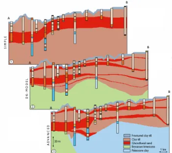
Fig. 1. Geological complexity and simulated age distribution. In a simple (upper), in an intermediary (middle), and in a complex hydrogeological conceptual model (lower). From Troldborg (2000).
transport and travel times the three models differed dramat-ically. When assessing the uncertainty contributed by the model parameter values using Monte Carlo simulations, the overlap of uncertainty ranges between the three models by Højberg and Refsgaard (2005) significantly decreased when moving from groundwater heads to capture zones and travel times. The larger the degree of extrapolation, the more the underlying conceptual model dominates over the parameter uncertainty and the effect of calibration. However, the pa-rameter uncertainty can not compensate for the variability (uncertainty) in the geological model structure.
The importance of geological interpretations on ground-water flow and age (particle tracking) predictions have been studied by Troldborg (2000, 2004). Using a zonation ap-proach three different conceptual models were constructed based on an extensive borehole database (Fig. 1). The three models differed in complexity. Calibrations of the models were performed using inverse calibration against hydraulic head and discharge measurements. Numerical simulation of groundwater age was carried out using a particle track-ing model. Although the three models provided very similar calibration fits to groundwater heads, a model extrapolation to predictions of groundwater ages revealed very significant differences between the three models, which were explained by the differences in underlying hydrogeological interpreta-tions.
Conditional geostatistical simulations is frequently used to address issues related to spatial distribution of conductivity (de Marsily et al., 1998; Kupfersberger and Deutsch, 1999). Most frequently, though, it is used after conceptualization
Fig. 2. Relationship between the geometric mean measured hy-draulic conductivity and the support volume (sample size) for differ-ent field measuremdiffer-ent methods in coarse-grained fluvial sedimdiffer-ents in Wisconsin. From Bradbury and Muldoon (1990).
of aquifer structures to generate conditional realizations of conductivity within hydrological units (facies) e.g. input for Monte Carlo analysis. A good example of this is found in Zimmerman et al.(1998), where they compared seven dif-ferent geostatistical approaches in combination with inverse modelling to simulate travel times and travel paths of conser-vative tracer through four synthetic aquifer data sets.
Geostatistical methods that can simulate hydrofacies dis-tributions at different scale are divided into structural and process imitating methods (Koltermann and Gorelick, 1996). De Marsily et al. (1998) point out that process imitating methods cannot be conditioned to local available informa-tion. Carle and Fogg (1996 and 1997) present a transition probability geostatistical framework that can be conditioned to hard as well as soft data in simulating hydrofacies distri-butions. There are several examples on application which include simulation of alluvial fan systems (Fogg et al., 1998; Weissmann et al., 1999; Weissmann and Fogg, 1999), river valley aquifer systems (Ritzi et al., 1994; Ritzi et al., 2000), Quaternary aquifer complex (Troldborg et al., 20071) and sandlenses distribution within glacial till in (Sminchak et al., 1996; Petersen et al., 2004).
Neuman and Wieranga (2002) present a generic strat-egy that embodies a systematically and comprehensive multiple conceptual model approach, including hydroge-ological conceptualisation, model development and pre-dictive uncertainty analysis. The strategy encourages an iterative approach to modelling, whereby an initial
1Troldborg, L., Refsgaard, J. C., Jensen, K. H., Engesgaard, P.,
Table 1. Classification of scales of sedimentary heterogeneity (From Koltermann and Gorelick, 1996).
Scale name: Basin Depositional environ-ments
Channels Stratigraphical features Flow regime features Pores
Approximate length scale
3 km–>100 km 80 m–3 km 5 m–80 m 0.1 m–5 m 2 mm–0.1 m <2 mm Geologic features Basin geometry, strata
geometries, structural features, lithofacies, regional facies trends
Multiple facies, facies relations, morphologic features
Channel geometry, bed-ding type and extent, lithology, fossil content
Abundance of sedimen-tary structures, stratifi-cation type, upward fin-ing/or coarsening
Primary sedimentary structures: ripples, cross-bedding, parting lineation, lamination, soft sediment deforma-tion
Grain size, shape, sort-ing, packing, orienta-tion, composiorienta-tion, ce-ments, interstitial clays
Heterogeneity affected by
Faults (sealing) folding, External controls (tec-tonic, sea level, cli-matic history), thickness trends, unconformities
Fractures (open or tight), intra-basinal controls (on fluid dynamics and depo-sitional mechanism)
Frequency of shale beds, sand and shale body ge-ometries, sediment load composition
Bed boundaries, minor channels, bars, dunes
Uneven diagenetic pro-cesses, sediment trans-port mechanisms, biotur-bation
Provenance, diagene-sis, sediment transport mechanisms
Observations/ measurement tech-niques
Maps, seismic profiles, cross-sections
Maps, cross-sections, lithologic and geo-physical logs, seismic profiles
Outcrop, cross-well to-mography, lithologic and geophysical logs
Outcrop, lithologic and geophysical logs
Core plug, hand sample, outcrop
Thin section, hand lens, individual clast, aggre-gate analysis
Support volume of hydraulic measure-ments
Shallow crustal proper-ties
Regional (long term pumping or tracer tests)
Local (short term pump-ing or tracer tests)
Near-well (non-pumping tests-height of screened interval)
Core plug analysis (per-meameter)
Several pores (mini-permeameter)
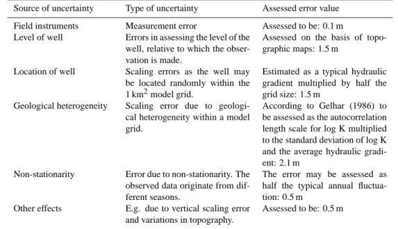
Table 2. The sources of uncertainty on groundwater head values and the assessed error values in this respect. Modified from Sonnenborg (2001).
Source of uncertainty Type of uncertainty Assessed error value
Field instruments Measurement error Assessed to be: 0.1 m
Level of well Errors in assessing the level of the well, relative to which the obser-vation is made.
Assessed on the basis of topo-graphic maps: 1.5 m
Location of well Scaling errors as the well may be located randomly within the 1 km2model grid.
Estimated as a typical hydraulic gradient multiplied by half the grid size: 1.5 m
Geological heterogeneity Scaling error due to geologi-cal heterogeneity within a model grid.
According to Gelhar (1986) to be assessed as the autocorrelation length scale for log K multiplied to the standard deviation of log K and the average hydraulic gradi-ent: 2.1 m
Non-stationarity Error due to non-stationarity. The observed data originate from dif-ferent seasons.
The error may be assessed as half the typical annual fluctua-tion: 0.5 m
Other effects E.g. due to vertical scaling error and variations in topography.
Assessed to be: 0.5 m
conceptual-mathematical model is gradually altered and/or refined until one or more likely alternatives have been iden-tified and analysed.
Professionals within the discipline have not yet agreed upon a procedure for ranking or weighting conceptual mod-els. Poeter and Anderson (2005) introduce a multimodel ranking and interference, which is a simple and effective ap-proach for the selection of a best model: one that balances under fitting with over fitting. Neuman and Wierenga (2003) propose and apply the Maximum Likelihood Bayesian Av-eraging (MLBA) approach for assessment of the joint
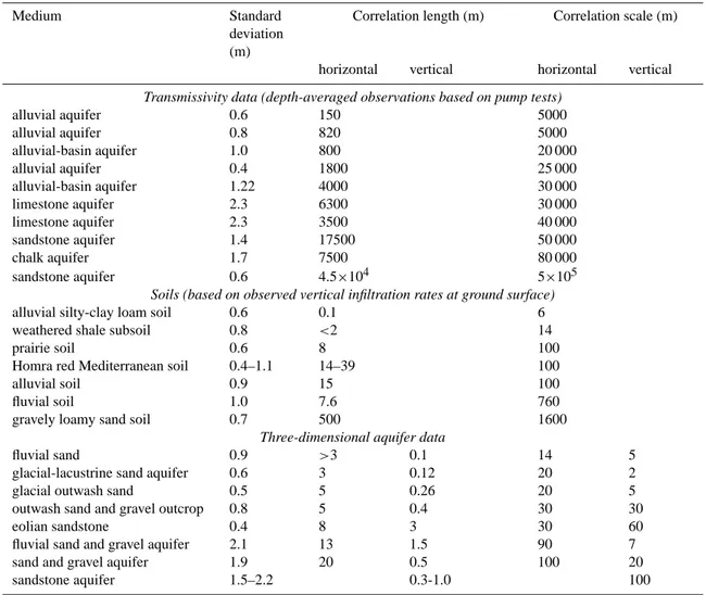
Table 3. Data on variance and correlation scales of the natural logarithm of hydraulic conductivity or transmissivity (From Gelhar, 1993).
Medium Standard
deviation (m)
Correlation length (m) Correlation scale (m)
horizontal vertical horizontal vertical
Transmissivity data (depth-averaged observations based on pump tests)
alluvial aquifer 0.6 150 5000
alluvial aquifer 0.8 820 5000
alluvial-basin aquifer 1.0 800 20 000
alluvial aquifer 0.4 1800 25 000
alluvial-basin aquifer 1.22 4000 30 000
limestone aquifer 2.3 6300 30 000
limestone aquifer 2.3 3500 40 000
sandstone aquifer 1.4 17500 50 000
chalk aquifer 1.7 7500 80 000
sandstone aquifer 0.6 4.5×10⁴ 5×10⁵
Soils (based on observed vertical infiltration rates at ground surface)
alluvial silty-clay loam soil 0.6 0.1 6
weathered shale subsoil 0.8 <2 14
prairie soil 0.6 8 100
Homra red Mediterranean soil 0.4–1.1 14–39 100
alluvial soil 0.9 15 100
fluvial soil 1.0 7.6 760
gravely loamy sand soil 0.7 500 1600
Three-dimensional aquifer data
fluvial sand 0.9 >3 0.1 14 5
glacial-lacustrine sand aquifer 0.6 3 0.12 20 2
glacial outwash sand 0.5 5 0.26 20 5
outwash sand and gravel outcrop 0.8 5 0.4 30 30
eolian sandstone 0.4 8 3 30 60
fluvial sand and gravel aquifer 2.1 13 1.5 90 7
sand and gravel aquifer 1.9 20 0.5 100 20
sandstone aquifer 1.5–2.2 0.3-1.0 100
3 Uncertainty in hydrogeological data
3.1 Scaling issues
One of the great and very general challenges within the hy-drological science is to understand the impact of changing scales on various process descriptions and parameter values. The average volume of hydrogeological measurements (also named support volume) is ranging many orders of magnitude depending on the size of volume representing the individual measurements. Spatial heterogeneity as a function of scale is well documented in the literature for saturated hydraulic con-ductivity (Clauser, 1992, S´anchez-Vila et al., 1996; Nilsson et al., 2001). Values of the saturated hydraulic conductivity depend on the volume of substrate sampled by the applied hydraulic testing method. A literature example in coarse-grained fluvial sediments (Bradbury and Muldoon, 1990) is shown in Fig. 2. It is evident that the mean hydraulic conduc-tivity increases as the support volume of the tests increases.
Aquifers contain many scales of hydrofacies or hydro-geological facies, which controls the hydraulic conductiv-ity structure. The descriptive nature of many classifications makes them somewhat subjective; however, they provide a useful basis for comparison between multiple scales of geo-logical heterogeneity (Koltermann and Gorelick, 1996) (Ta-ble 1). Scales of geological and hydraulic conductivity struc-ture are based on (a) size of the geological feastruc-tures, (b) ge-netic origin, (c) support length (porous media measurement volumes).
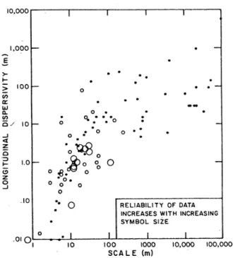
Fig. 3. Longitudinal dispersivity data plotted versus scale of exper-iment; the largest symbols indicate the most reliable data. (Gelhar, 1986).
scale value representing a small time scale (e.g. 10 s) should be upscaled to show its representativeness of an average an-nual value, taking the seasonal variations into account. The sources of uncertainty and their respective contributions in this respect are shown in Table 2. Assuming mutual inde-pendence between these individual errors the aggregated un-certainty of the observed head data relative to model simula-tions at a 1 km2scale can be estimated as the square root of the sum of the squared errors, summing up to 3.1 m. 3.2 Variability on hydraulic properties
Data on spatial variability investigated by means of geosta-tistical methods have obtained significant attention in the scientific literature (Isaaks and Srivastava, 1989). For all practical purposes at the time scales relevant for this paper the variables are considered invariant. Several studies have focused on the determination of spatial correlation length scales for different hydraulic properties (e.g. Dagan, 1986; Gelhar, 1993). Variability becomes uncertain because it can-not be captured by direct field or laboratory measurements. Instead, the parameter variability is recognised by the geosta-tistical measure like mean, variance and correlation length. 3.2.1 Hydraulic conductivity (K)
Gelhar (1993) summarise the standard deviation and correla-tion lengths (λ)of hydraulic conductivity from several field studies in Table 3, which covers a wide range of field scales
Table 4. Value ranges of effective porosity (n), specific yield (Sy)
and specific storage (Ss). Data sources: a) Freeze and Cherry
(1979), b) Anderson (1989), and c) Smith and Weathcroft (1992).
Material na) Syb+c) Ssb+c)
Gravel 25–40 0.2–0.4 10−4–10−6
Sand 25-50 0.1-0.3 10−3–10−5
Clay 40–70 0.01–0.1 10−3–10−4
Sand and gravel 20–35 0.15-0.25 10−3–10−4
Sandstone 5–30 0.05–0.15 10−3–10−5
Limestone 0–20 0.005–0.05 10−3–10−5
Shale 0-10 0.005-0.05 10−3–10−5
and seems to indicate that the length scale of field data for which correlation length and standard deviation have been assessed increases with increasing field scale.
Different measurement techniques used to determine satu-rated hydraulic conductivity representing 13 orders of magni-tude in a coarse-grained fluvial material are shown in Fig. 2. The hydraulic conductivity of various geological materials is ranging multiple orders of magnitude with unfractured bedrocks and matrix permeability in glacial tills in the lower end and unconsolidated sediments in the middle to upper end. 3.2.2 Storage coefficients, effective porosity and
dispersiv-ity
Correlation lengths of specific yield (Sy), specific storage
(Ss)and effective porosity (n) are not found in the literature.
The range of values related to different soil types are avail-able (Tavail-able 4). The longitudinal dispersivity (α) has been compiled in Fig. 3 from many field sites with very different geological setting around the world (Gelhar, 1986). These data indicates that a longitudinal dispersivity in the range of 1 to 10 m would be reasonable for a site of dimensions on the order of 1 km, whereas the range of 10 to 1000 m would cover the river basin length scale on the order of few km to more than 100 km. The dispersivity value typically varies by 2 to 3 orders of magnitude depending on which length that are of interest.
3.3 Classification of data uncertainty in accordance to Har-moniRiB terminology and classes
As part of the data processing the HarmoniRiB project part-ners have characterised and assessed the data uncertainty us-ing the new methodology described by Brown et al. (2005) and using the DUE (Data Uncertainty Engine) software tool (Brown and Heuvelink, 2006). This new methodology has been further elaborated in van Loon and Refsgaard (2005).
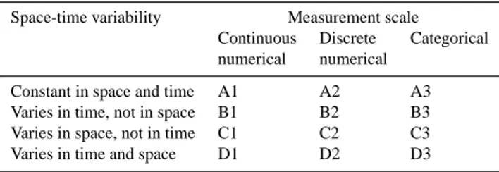
Table 5. The subdivision and coding of attribute uncertainty-categories, along the “axes” of space-time variability and measure-ment scale (van Loon and Refsgaard, 2005).
Space-time variability Measurement scale Continuous Discrete Categorical numerical numerical
Constant in space and time A1 A2 A3 Varies in time, not in space B1 B2 B3 Varies in space, not in time C1 C2 C3 Varies in time and space D1 D2 D3
Table 6. Types of empirical uncertainty (van Loon and Refsgaard, 2005).
Code Explanation
M1 Probability distribution or upper & lower bounds M2 Qualitative indication of uncertainty
M3 Some examples of different values a variable may take
various fields of hydrology without being overly complex. The methodology is based on a distinction between the em-pirical quality of data and the sources of uncertainty in data. 3.3.1 Attribute, empirical and longevity uncertainty By considering space-time variability and data type 13 uncer-tainty categories of uncertain data are distinguished between (Table 5). In addition it is useful to distinguish the meth-ods for describing uncertainty, which depend on the type and amount of information available (Table 6). The source of uncertainty related to relative age (denoted by the term “longevity”) has been given in Table 7. Often, the identi-fication of sources of uncertainty, such as instrument accu-racy, errors due to under-sampling or differences in defini-tions, help in properly identifying the category or probability distribution function (pdf) of empirical uncertainty (Table 8). Tables 5–8 show the key characteristics used to characterise data uncertainty in the following hydrogeological variables.
The specific yield, effective porosity and dispersivity are all assessed to typically have a measurement space support of about 100 cm3. Hydraulic conductivity and specific storage have a measurement space support scale ranging from 10−5
to 109m3depending on sample size of the applied method to determine the variable. The uncertainty category is for all variables classified as C1 (cf. Table 5), which means that they are assumed to vary continuously in space but not in time. The type of empirical uncertainty is classified as M1 (Table 6) for all five parameters implying that uncertainty can be characterised statistically by use of probability den-sity functions. The relative age of uncertainty description is
Table 7. Codes for “longevity’; of uncertainty information (van Loon and Refsgaard, 2005).
Code Explanation
L0 Temporal variability of the uncertainty information is unknown.
L1 The uncertainty information is known to change significantly over time (specify how fast it changes if you know it).
L2 Uncertainty does not change significantly, in principle no updating required.
classified as L2 (Table 7) for all variables, which means the uncertainty does not change significantly so no updating is required.
3.3.2 Methodological quality uncertainty
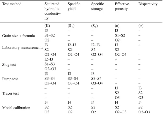
Based on the simplified descriptions of the methodological quality uncertainty in Table 8 by Brown et al. (2005), has the methodological quality of commonly employed test methods for determination of hydrogeological parameters been char-acterised as given in Table 9.
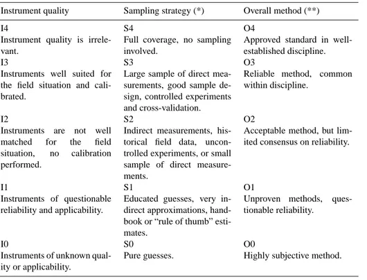
Table 8. Indices for “methodological quality” of a variable. (*) One may specify the sampling strategy in the different spatial dimensions (Ss = in space, Sh = horizontal, Sv = Vertical), and also in time (St). (**) Under “overall” method’ we group the combined and described procedures to collect/transport/process/calculate the variable of interest. (From van Loon and Refsgaard, 2005).
Instrument quality Sampling strategy (*) Overall method (**)
I4
Instrument quality is irrele-vant.
S4
Full coverage, no sampling involved.
O4
Approved standard in well-established discipline. I3
Instruments well suited for the field situation and cali-brated.
S3
Large sample of direct mea-surements, good sample de-sign, controlled experiments and cross-validation.
O3
Reliable method, common within discipline.
I2
Instruments are not well matched for the field situation, no calibration performed.
S2
Indirect measurements, his-torical field data, uncon-trolled experiments, or small sample of direct measure-ments.
O2
Acceptable method, but lim-ited consensus on reliability.
I1
Instruments of questionable reliability and applicability.
S1
Educated guesses, very in-direct approximations, hand-book or “rule of thumb” esti-mates.
O1
Unproven methods, ques-tionable reliability.
I0
Instruments of unknown qual-ity or applicabilqual-ity.
S0
Pure guesses.
O0
Highly subjective method.
Specific yield (Sy) : Retention curve determinations on
laboratory scale have instrument quality range from not well to well match of the field conditions. Keur and Vangsø (this HESS issue) describe more thoroughly the application of re-tention curves to determination of physical parameters on various scales. Pump tests have the highest instrument qual-ity, best coverage of sampling strategy and is an overall reli-able method. Model calibration is commonly used and seen as an acceptable method for Syestimation but there is limited
consensus on the reliability of the results.
Specific storage (Ss)has been characterised with the same
indices ranking as Sy but on laboratory scale are retentions
curves exchanged with geotechnical triaxial tests to deter-mine specific storage.
Effective porosity (n): This variable has the instrument quality well suited at both small and large scale. All test methods are ranking between educated guesses to indirect measurements. Results derived from tracer tests can among others be used for effective porosity estimation. All test methods are grouped as acceptable methods even with some specific methods appearing as approved standards for poros-ity measuring.
Dispersivity (α): The alpha value is limited to be deter-mined from the larger scale methods: tracer test and model calibration.
In general, the HarmoniRiB framework indices for the methodological quality increase with increasing support vol-ume, which the different test methods represent. Individual indices show higher variability at small scale test methods compared to larger scale methods due to effects of spatial scale.
4 Discussion and conclusions
Uncertainty assessment is an important aspect of water re-sources management. First of all, water management deci-sions should be made with full information on the underly-ing uncertainties. Secondly, credibility of model predictions among stakeholders is important for achieving consensus and robust decisions. Overselling of model capabilities is “poi-son” for establishing such credibility. Instead, explicit in-formation on the involved uncertainties may help creating a more balanced view on the capability of models and in this way pave the road for improving the credibility of models.
Table 9. Methodological quality: Instrument quality (I); Sampling strategy (S) and Overall method (O). –: test method not common/relevant for determination of specific hydraulic parameter values.
Test method Saturated
hydraulic conductiv-ity
Specific yield
Specific storage
Effective porosity
Dispersivity
(K) (Sy) (Ss) (n) (α)
Grain size + formula
I3 – – I3 –
S1–S2 – – S1–S2 –
O2 – – O2 –
Laboratory measurementsI3 I2–I3 I2–I3 I3 –
S2 S2 S2 S2 –
O2–O4 O2–O4 O2–O4 O2–O4 –
Slug test
I2–I3 – – – –
S1–S3 – – – –
O2–O3 – – – –
Pump test
I3 I3 I3 – –
S3–S4 S3–S4 S3–S4 – –
O3–O4 O3–O4 O3–O4 – –
Tracer test
– – – I3 I3
– – – S2 S2
– – – O3 O3
Model calibration
I4 I4 I4 I4 I4
S2 S2 S2 S2 S2
O3 O2 O2 O2–O3 O2–O3
management. We therefore have a major task in promoting the use of our uncertainty concepts and tools in practise.
In this paper, examples from the most current scientific literature that deal with uncertainty on model structure and uncertainty in parameter variables are given. Quantification of the uncertainty due to model structure is an area of novel interest, where only few operational methods have been de-veloped. Some of the present techniques to describe the un-certainty related to geological model structure are presented and some strategies on interpretation of geological model structure are identified. In addition, uncertainty and scale of support in the hydrogeological data variables: saturated hy-draulic conductivity, specific yield, specific storage, effective porosity and dispersivity are evaluated. The variables are re-lated to the following test methods: grain size analysis, other laboratory measurements, slug tests, pump tests, tracer tests and model calibrations.
Uncertainty in the hydrogeological data variables is in this study characterised and assessed within the methodological framework of the HarmoniRiB classification, where the rat-ing of the quality of methods can be given in a more struc-tured overview. In general, the HarmoniRiB framework in-dices for the methodological quality increase with increas-ing support volume, which the different test methods rep-resent. Individual indices shows higher variability at small scale test methods compared to larger scale methods due to
effects of spatial scale. The use of the HarmoniRiB classi-fication makes it possible to carry out systematic compari-son of uncertainties arising in different data types required for evaluating the effect and cost of a measure in relation to preparing a water management plan in relation to the EU Water Framework Directive.
have a major challenge in developing and testing concepts for handling model structure uncertainty, and to make best possible use of qualitative geological knowledge in this con-text.
Acknowledgements. The present work was carried out within the Project “Harmonised Techniques and Representative River Basin Data for Assessment and Use of Uncertainty Information in Inte-grated Water Management (HarmoniRiB)”, which is partly funded by the EC Energy, Environment and Sustainable Development programme (Contract EVK1-CT2002-00109)
Edited by: J. Freer
References
Anderson, M. P.: Hydrogeologic facies models to delineate large-scale spatial trends in glacial and glaciofluvial sediments, Geo-logical Society America Bulletin, 101, 501–511, 1989.
Anderson, M. P. and Woessner, W. W.: Applied groundwater mod-elling, simulation of flow and advective transport. Academic Press, San Diego, California, 1992
Bersezio, R., Bini, A., and Giudici, M.: Effects of sedimentary het-erogeneity on groundwater flow in a Quaternary pro-glacial delta environment: joining facies analysis and numerical modelling, Sedimentary Geology, 129, 327–344, 1999.
Bradbury, K .R. and Muldoon, M. A.: Hydraulic conductivity de-termination in lithified glacial and fluvial materials, In: Ground Water and Vadose Zone Monitoring, ASTM STP 1053, edited by: Nielsen, D. M. and Johnsen, A. I., American Society for test-ing Materials, Philadelphia, 138–151, 1990.
Brown, J. D., Heuvelink, G. B. M., and Refsgaard, J. C.: An inte-grated framework for assessing and recording uncertainties about environmental data, Water Sci. Technol., 52(6), 153–160, 2005. Brown JD and Heuvelink GBM: Data Uncertainty Engine
(DUE) User’s Manual. University of Amsterdam. http://www. harmonirib.com, 2006.
Carrera, J. and Neuman, S. P.: Estimation of aquifers parameters un-der transient and steady state conditions: 1. Maximum likelihood method incorporating prior information, Water Resour. Res., 22, 199–210, 1986.
Carle, S. F. and Fogg, G. E.: Transition probability based on indi-cator geostatistics, Mathematical Geology, 28, 453–477, 1996. Carle, S. F. and Fogg, G. E.: Modelling spatial variability with one
and multidimensional continuous-lag Markov chains, Mathemat-ical Geology, 29, 891–917, 1997.
Clauser, C.: Permeability of crystalline rocks, Eos 73, 233–238, 1992.
Cooley, R. L.: A theory for modelling ground-water flow in hetero-geneous media. U.S.G.S. Professional Paper, vol. P 1679. U.S. Geological Survey, Denver, CO, 220 pp., 2004.
Dagan, G.: Statistical theory of groundwater flow and transport: Pore to laboratory, laboratory to formation and formation to re-gional scale, Water Resour. Res., 22(9), 120S–134S, 1986. Dagan, G., Fiori, A., and Jankovi, I.: Flow and transport in highly
heterogeneous formations : 1. Conceptual framework and valid-ity of first-order approximations, Water Resour. Res., 39, 1268, doi:10.1029/2002WR001717, 2003.
de Marsily, G., Delay, F., Teles, V., and Schafmeister, M. T.: Some current methods to represent the heterogeneity of natural media in hydrogeology, Hydrogeol. J., 6(1), 115–130, 1998.
Eaton, T.: On the importance of geological heterogeneity for flow simulation, Sedimentary Geology, 184, 187–201, 2006. European Commission: EU Water Framework Directive
(Direc-tive 2000/60/EC). European Parliament and Commission, Offi-cial Journal (OJ L 327) on 22 December 2000.
Fogg, G. E.: Groundwater flow and sand body interconnectedness in a thick multiple aquifer system, Water Resour. Res., 22, 679– 694, 1986.
Fogg, G. E., Noyes, C. D., and Carle, S. F.: Geologically based model of heterogeneous hydraulic conductivity in an alluvial set-ting, Hydrogeol. J., 6(1), 131–143, 1998.
Fraser, G. S. and Davis, J. M. (Eds.): Hydrogeologic models of sed-imentary aquifers, SEPM Concepts in Hydrology and Environ-mental geology, vol. 1. Society for Sedimentary Geology, Tulsa, OK. 180 pp., 1998.
Freeze, R. A. and Cherry, J. A.: Groundwater. Prentice Hall, Engle-wood Cliffs, NJ 07632, USA, 1979.
Funtowicz, S. O. and Ravetz, J. R.: Uncertainty and Quality in Sci-ence for Policy. Kluwer, Dordrecht; 229 p., 1990.
Gelhar, L. W.: Stochastic subsurface hydrology from theory to ap-plication, Water Resour. Res., 22(9), 135S–145S, 1986. Gelhar, L. W.: Stochastic subsurface hydrology, Englewood Cliffs,
NJ, Prentice Hall, 1993.
Harrar, W. G., Sonnenborg, T. O., and Henriksen, H. J.: Capture zone, travel time and solute transport predictions using inverse modelling and different geological models, Hydrogeol. J., 11, 536–548, 2003.
Henriksen, H. J., Troldborg, L., Nyegaard, P., Sonnenborg, T. O., Refsgaard, J. C., and Madsen, B.: Methodology for construction, calibration and validation of a national hydrological model for Denmark, J. Hydrol., 280, 52–71, 2003.
Højberg, A. L. and Refsgaard, J. C.: Model Uncertainty - Param-eter uncertainty versus conceptual models, Water Sci. Technol., 52(6), 177–186, 2005.
Isaaks, E. D. and Srivastava, R. M.: An Introduction to Applied Geostatistics. Oxford University Press, New York, USA, 1989. Klingbeil, R., Kleineidam, S., Asprion, U., Aigner, T., and Teutsch,
G.: Relating lithofacies to hydrofacies: Out-crop hydrogeologi-cal characterization of Quaternary gravel deposits, Sedimentary Geology, 129, 299–310, 1999.
Koltermann, C. E. and Gorelick, S. M.: Heterogeneity in sedimen-tary deposits: A review of structure-imitating, process-imitating and descriptive approaches, Water Resour. Res., 32, 2617–2658, 1996.
Kupfersberger, H. and Deutsch, C. V.: Ranking stochastic realiza-tions for improved aquifer response uncertainty assessment, J. Hydrol., 223(1–2), 54–65, 1999.
National Research Council: Conceptual models of flow and trans-port in vadose zone. National Academy Press, Washington, DC., 2001.
Neuman, S. P. and Weirenga, P. J.: A comprehensive strategy of hydrogeologic modelling and uncertainty analysis for nuclear fa-cilities and sites, NUREG/CR-6805, 2003.
162–179, 2001.
Petersen, D. L., Jensen, K. H., and Nilsson, B.: Effect of embed-ded sand lenses on transport in till. Eos, Transactions, American Geophysical Union, 85(47), Fall Meeting, 2004.
Poeter, E. M. and Anderson, D.: Multimodel ranking and inference in ground water modelling, Groundwater, 43(4), 597–605, 2005. Poeter, E. M. and Hill, M. C.: Inverse methods: A necessary next step in ground water modelling, Groundwater, 35(2), 250–260, 1997.
Refsgaard, J. C., Nilsson, B., Brown, J., Klauer, B., Moore, R., Bech, T., Vurro, M., Blind, M., Castilla, G., Tsanis, I., and Biza, P: Harmonised Techniques and Representative River Basin Data for Assessment and Use of Uncertainty Information in Integrated Water Management (HarmoniRiB), Environmental Science and Policy, 8, 267–277, 2005.
Refsgaard, J. C., van der Sluijs, J. P., Brown, J., and van der Keur, P.: A framework for dealing with uncertainty due to model structure error, Adv. Water Resour., 29(11), 1586–1597, 2007a.
Refsgaard, J. C., van der Keur, P, Nilsson, B., M¨uller-Wohlfeil, D.-I., and Brown, J.: Uncertainties in river basin data at various sup-port scales – examples from Odense Pilot River Basin, Hydrol. Earth Syst. Sci. Discuss., 3, 1943–1985, 2006b.
Ritzi Jr., R. W., Dominic, D. F., Slesers, A. J., Greer, C. B., Re-boulet, E. C., Telford, J. A., Masters, R. W., Klohe, C. A., Bogle, J. L., and Means, B. P.: Comparing statistical models of physical heterogeneity in buried-valley aquifers, Water Res. Res., 36(11), 3179–3192, 2000.
Ritzi, R. W., Jayne, D. F., Zahradink, A. J., Field, A. A., and Fogg, G. E.: Geostatistical modeling of heterogeneity in glaciofluvial, buried-valley aquifers, Ground Water, 32(4), 666–674, 1994. Rode, M. and Suhr, U.: Uncertainties in selected surface water
qual-ity data, Hydrol. Earth Syst. Sci. Discuss., 3, 2991–3021, 2006, http://www.hydrol-earth-syst-sci-discuss.net/3/2991/2006/. Samper, J., Carrera, J., Galarza, G., and Medina, A.: Application
of an automatic calicration technique to modelling an alluvial aquifer, IAHS AISH Publication, 195, 87–95, 1990.
S´anchez-Vila, X., Girardi, J., and Carrera, J.: Scale effects in trans-missivity, J. Hydrol., 183, 1–22, 1996.
Selroos, J. O., Walker, D. D., Strom, A., Gylling, B., and Follin, S.: Comparison of alternative modelling approaches for groundwa-ter flow in fractured rock, J. Hydrol., 257, 174–188, 2001. Sminchak, J. R., Dominic, D. F., and Ritzi, R. W.: Indicator
geo-statistical analysis of sand interconnections within a till, Ground Water, 34(6), 1125–1131, 1996.
Smith, L. and Weathcroft, S. W.: Groundwater flow In: Maidment DR (Ed. in chief), Handbook of Hydrology, Mc Graw-Hill Inc., 1992.
Sonnenborg, T. O.: Kalibrering af strømningsmodel, in: St˚abi i grundvandsmodellering, edited by: Henriksen, H. J., Refsgarrd, J. C., Sonnenborg, T. O., et al., GEUS report, No. 56, 2001. Troldborg, L.: Effects of geological complexity on groundwater
age prediction, Eos, Transactions, American Geophysical Union, 81(48), F435, 2000.
Troldborg, L.: The influence of conceptual geological models on the simulation of flow and transport in Quaternary aquifer systems. PhD. Thesis. Geological Survey of Denmark and Greenland, Re-port 2004/107, 2004.
van der Keur, P. and Iversen, B. V.: Uncertainty in soil physical data at river basin scale – a review, Hydrol. Earth Syst. Sci., 10, 889– 902, 2006,
http://www.hydrol-earth-syst-sci.net/10/889/2006/.
van Loon, E. and Refsgaard, J. C. (Eds.): Guidelines for assess-ing data uncertainty in hydrological studies. HarmoniRiB Re-port. Geological Survey of Denmark and Greenland, http://www. harmonirib.com, 2005.
van Loon, E., Brown, J. D., and Heuvelink, G. M. B.: Metodologi-cal Considerations. Chapter 2 in: 2005. Guidelines for assessing data uncertainty in hydrological studies, edited by: Van Loon, E. and Refsgaard, J. C., HarmoniRiB Report. Geological Survey of Denmark and Greenland, http://www.harmonirib.com, 2005. Weissmann, G. S., Carle, S. F. and Fogg, G. E.: Three dimensional
hydrofacies modeling based on soil surveys and transition proba-bility geostatistics, Water Resour. Res., 35(6), 1761–1770, 1999. Weissmann, G. S. and Fogg, G. E.: Multi-scale alluvial fan het-erogeneity modelled with transition probability geostatistics in a sequence stratigraphic framework, J. Hydrol., 226(1–2), 48–65, 1999.
Willis, B. J. and White, C. D.: Quantitative outcrop data for flow simulation, J. Sedimentary Res., 70(4), 788–802, 2000. Zimmerman, D. A., de Marsily, G., Gotway, C. A., Marietta, M. G.,