Surveys of Young Stars: Variability and Binarity
Marcelo Medeiros Guimar˜aes
MARCELO MEDEIROS GUIMAR ˜AES
Surveys of Young Stars: Variability and Binarity
Tese apresentada `a UNIVERSIDADE FEDERAL DE MINAS GERAIS como requisito parcial para obten¸c˜ao do grau de DOUTOR EM F´ISICA
Orientador: Prof. Luiz Paulo Ribeiro Vaz Co-orientador: Prof. Bo Reipurth
Departamento de F´ısica - ICEx - UFMG
Agradecimentos
A ciˆencia exige dedica¸c˜ao exclusiva daquele que a estuda. Por vezes o cientista sai de seu laborat´orio e leva consigo os problemas que ainda teimam em n˜ao ser solucionados. Dorme pensando neles, algumas vezes esses problemas s˜ao resolvidos em sonhos, outras vezes eles requerem anos de intenso e ´arduo trabalho. Por isso ´e necess´ario ter paix˜ao pelo que se faz. Por isso fazemos ciˆencia, porque depois de longas horas, `as vezes dias, semanas, o resultado nos salta aos olhos e um sorriso nos vem ao rosto.
Eu tive a sorte de ter trabalhado, durante o meu doutorado, com dois exemplos claros de dedica¸c˜ao `a ciˆencia. Luiz Paulo e Bo, cada um `a sua maneira, dedicam suas carreiras em prol do avan¸co da ciˆencia. Com Luiz Paulo aprendi a ter muito cuidado com os detalhes do trabalho. Sempre ter certeza de como as coisas funcionam, nunca confiar em “caixas pretas”. Bo me mostrou o lado apaixonante da ciˆencia, me mostrou que ´e necess´ario ter for¸ca de vontade para seguir em frente. Espero ter aprendido o suficiente com eles para poder tamb´em fazer contribui¸c˜oes relevantes para o avan¸co da astronomia. Sou muito grato a eles por tudo que me ensinaram e por seus exemplos.
Uma vida dedicada `a ciˆencia requer sacrif´ıcios, que seriam muito piores n˜ao fosse o apoio constante da fam´ılia, da namorada e dos amigos. Felizmente sempre recebi muito apoio das pessoas a minha volta e sou muito grato a vocˆes por todo o amor, carinho, aten¸c˜ao, amizade e respeito. Muitas pessoas passaram pela minha vida ao longo desses anos, algumas partiram, outras ficaram, mas todas deixaram marcas que me fazem o que sou hoje. A todas elas, muito obrigado.
S´o com sacrif´ıcio n˜ao se faz ciˆencia, ´e necess´ario financiamento. Agrade¸co `as agˆencias financiadoras, CNPq e Capes, pelas bolsas de doutorado e doutorado sandu´ıche, que me per-mitiram realizar essa tese. Agrade¸co novamente ao meu co-orientador, Bo, pelo financiamento que me permitiu passar um ano trabalhando ao seu lado no Hava´ı e por ter me fornecido as observa¸c˜oes que s˜ao essenciais para essa tese. Tamb´em agrade¸co Andy Adamson por coordenar as observa¸c˜oes com o UKIRT e pelo seu apoio incans´avel a esse projeto.
Acknowledgements
Science demands exclusive dedication from those who study it. Many times the scientist leaves his laboratory and takes with him the problems that still insist not to be solved. He sleeps thinking about them, sometimes they are solved in his dreams, sometimes the problems require years of intense, hard work. That is why it is necessary to have passion for what one does. That is why we do science, because after long hours, sometimes days, weeks, the result jumps before our eyes and a smile comes to our face.
I was lucky I had the chance, during my PhD, to work with two clear examples of dedication to science. Luiz Paulo and Bo, each in his own way, dedicate their career to the development of science. I learned from Luiz Paulo to be careful about the details, to always be sure how things work and never trust “black boxes”. Bo showed me the passionate side of science and how it is necessary to have will power to keep going. I hope a have learned enough with them to also be able to make relevant contributions to the development of astronomy. I am very grateful to them for all they have taught me and their examples.
A life dedicated to science requires sacrifices, which would be worst if it were not for the constant support of the family, girlfriend and friends. Fortunately I have always received much support from the people around me and I am very grateful to you all for all the love, care, attention, friendship and respect. A lot of people were part of my life along these years, some have gone by, others remained, but all of them left marks which made me what I am today. To all of you, thank you very much.
Only sacrifice does not do science, financial support is necessary. I thank the supporting agencies, CNPq and Capes, for the fellowships that allowed me to develop this thesis. I thank again my co-advisor, Bo, for his financial support which allowed me to spent one year working by his side in Hawaii and also for providing the observations which are essential for this thesis. I also thank Andy Adamson for coordinating the UKIRT observations and for his tireless support of this project.
Content
RESUMO viii
ABSTRACT x
1 Introduction 1
2 Visual Binaries in the Orion Nebula Cluster 5
2.1 Introduction . . . 5
2.2 Observation and Catalogs . . . 7
2.3 Membership of the ONC . . . 10
2.4 Completeness . . . 11
2.5 Results . . . 17
2.5.1 Binary Fraction . . . 17
2.5.2 Separation Distribution Function . . . 18
2.5.3 Wide versus Close Binaries . . . 18
2.5.4 Flux Ratios and Substellar Companions . . . 21
2.6 Summary of Results . . . 23
2.7 Individual Binaries of Interest . . . 24
3 Variability 27 3.1 Introduction . . . 27
3.2 Types of Variables . . . 28
3.3 Statistical Indices . . . 28
3.4 Testing the Indices . . . 31
4 The Orion Nebula Survey 41 4.1 Introduction . . . 41
4.2 WFCAM Survey . . . 42
4.2.1 Problems . . . 42
4.2.2 Reduction . . . 45
4.3 Observations . . . 47
4.3.2 Superposition problems and calibration solutions . . . 49
4.4 Variable Candidates . . . 53
4.4.1 Eclipsing binary candidates . . . 53
4.4.2 Periodic variables . . . 54
4.4.3 Interesting light curves . . . 54
4.5 Summary of Results . . . 57
5 The Cygnus OB2 Survey 67 5.1 Introduction . . . 67
5.2 Observations . . . 71
5.3 Cometary Globules . . . 75
5.4 The Cygnus OB2 Center . . . 77
5.5 Infrared Sources . . . 78
5.5.1 IRAS 20321+4112 . . . 79
5.5.2 IRAS 20327+4120 . . . 80
5.5.3 IRAS 20332+4124 . . . 81
5.5.4 IRAS 20333+4127 . . . 82
5.5.5 DR18 . . . 82
5.5.6 IRAS 20304+4059 . . . 84
5.6 Summary of Results . . . 86
6 Conclusions 87 7 Resumo da Tese em Portuguˆes 90 7.1 Introdu¸c˜ao . . . 90
7.2 Bin´arias Visuais no Aglomerado da Nebulosa de ´Orion . . . 93
7.2.1 Introdu¸c˜ao . . . 93
7.2.2 Resultados . . . 94
7.3 ´Indices Estat´ısticos . . . 95
7.4 Levantamento Fotom´etrico da Nebulosa de ´Orion . . . 96
7.4.1 Introdu¸c˜ao . . . 96
7.4.2 Resultados . . . 97
7.5 Levantamento Fotom´etrico em Cygnus OB2 . . . 97
7.5.1 Introdu¸c˜ao . . . 97
7.5.2 Resultados . . . 98
7.6 Conclus˜oes . . . 98
List of Figures
2.1 Distribution of the visual binaries, with different separations, in the observed region. The grey solid circle, with a radius of 60′′
and centered in θ1 Ori C, is called the exclusion zone. We did not consider, in our analysis, any star inside this zone. Single stars are plotted as asterisks and binaries (triples included) are plotted as black filled circles. . . 8 2.2 Definition of the position angle (PA) and separation (S) between primary and
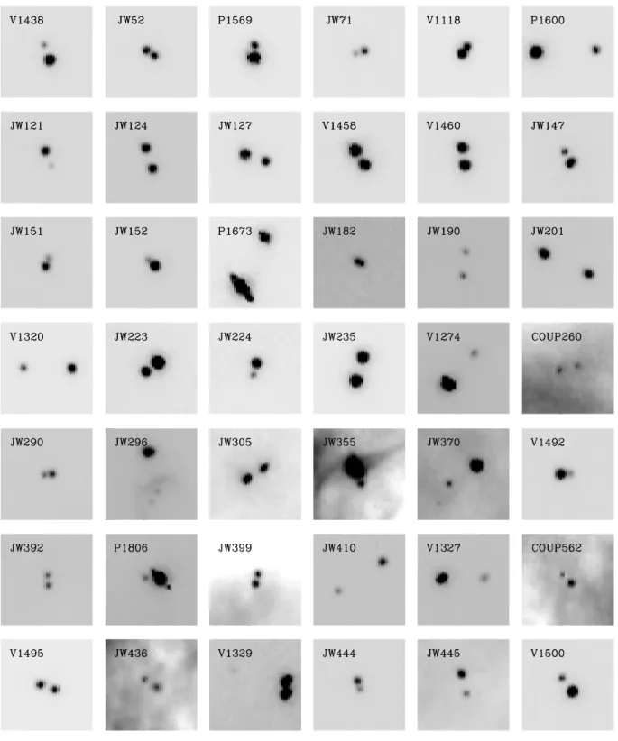
secondary in a binary system. . . 9 2.3 All binaries identified among the ONC members. Each stamp is 2′′
wide, with north pointing up and east pointing left. . . 12 2.3 Continued . . . 13 2.4 Examples of the artificial binaries, created using the profiles of real stars of our
sample, in order to analyse our completeness. . . 15 2.5 These two plots show the ∆m versus binary separation in arcseconds. The
observed binaries are shown in the left panel, where the dashed line indicates the 0′′.
15 separation limit. The right panel shows the artificial binaries, created from real stars present in our images, with different separations, position angles and ∆m. In the right panel, filled circles indicate systems where we could detect the companions, while open circles represent those where we were not able to detect them. . . 16
2.6 Left panel: surface density profile of the ONC members as a function of distance toθ1 Ori C. The exclusion zone is indicated by the dashed line. This profile was used as a guide to understand and localize the subclustering in the region studied. It was not used to obtain the probability of chance alignment. Right panel: probability that a star would have a companion as a line-of-sight association, obtained with Eq. (2.1). Presented here are all the 781 ONC members, squares for single stars and circles for binaries. One can see a subclustering around 180′′
. We used the surface density obtained considering the number of stars inside an area of 30′′
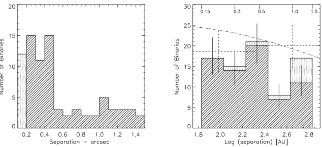
2.7 The left panel shows the histogram of binary angular separations in steps of 0′′. 1. The number of binaries in the innermost bin, with separations less than 0′′.1, is incomplete. We filled this bin with vertical dotted lines. One can see the abrupt decrease in the number of binaries when the separation increases beyond 0′′.
5. The right panel shows the logarithmic separation distribution function of the ONC binaries compared to the distribution of field binaries from Duquennoy & Mayor (1991) across the separation range from 0′′.
15 to 1′′.
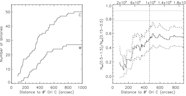
5. The dot-filled part of the histogram bins represents the contamination by line-of-sight pairs, obtained using Eq. (2.1). The bins representing large separations are the most contaminated ones, as expected. The vertical solid lines present in each bin represent the 1-σ errors calculated using a binomial distribution. The data from DM91 within our separation range are shown as two dashed crosses, while the Gaussian distribution they fit to their complete data set is represented by the dash-dotted line, which can be seen above the histogram. The top axis indicates separations in arcseconds at the distance of the ONC. . . 19 2.8 The left panel shows the cumulative distributions of close (0′′.15 – 0′′.5) and wide
(0′′. 5 – 1′′.
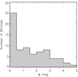
5) binaries in the ONC as a function of distance from θ1 Ori C. The right panel shows the ratio of wide to close binaries in the ONC as a function of distance toθ1 Ori C. The dashed lines indicate the errors. The dotted horizontal lines at the top of the panel are the same ratio from the DM91 field binary study. The lower line comes from their Gaussian fit and the upper line comes from their actual data points. The top axis scale shows the crossing time in years, assuming a mean one-dimensional velocity dispersion of 2 km s−1. The vertical dot-dashed line indicates the distance where the ratio becomes essentially flat, suggesting an age for the ONC of about 1Myr. . . 20 2.9 Luminosity ratio of the binary population, based on the Hα fluxes of primaries
and secondaries. All binaries with separation between 0′′.1 and 1′′.5 are plotted,
except the saturated ones. . . 21 2.10 R-band magnitudes as a function of spectral type for M dwarfs and very cool
objects (spectral type L). . . 22
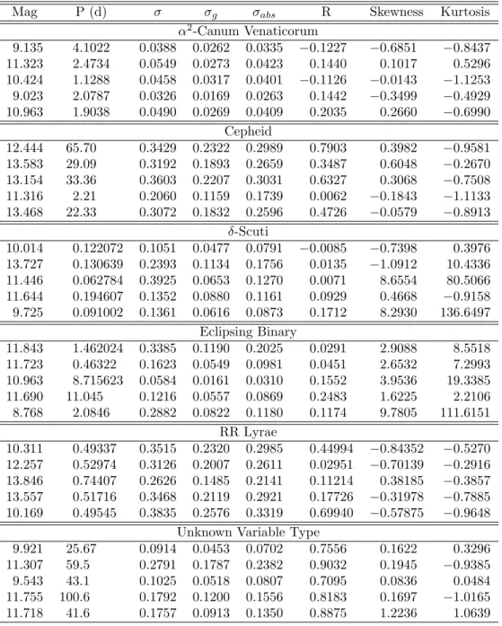
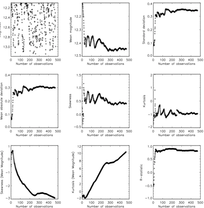
3.1 Examples of the light curves of the variables stars used to test the statistical indices. The plots show the star’s V magnitude versus the phase. The period, indicated in each panel in days, was obtained in the ASAS database. Each panel has a label at the top indicating the variable type; starting in the first row we have the α2 Canum Venaticorum (ACV), Cepheids (CEP), δ-Scuti (DSCT), eclipsing binary (EB), RR Lyrae (RR) and unknown type variable (Unk). . . 32 3.2 Statistical indices applied to an α2-Canum Venaticorum type star as a function
of time. In the first row we present, from left to right, the real light curve of the star, the Mean Magnitude curve and the σ-curve. The second row shows theσabs-curve, the skewness curve and the kurtosis curve. These last two curves
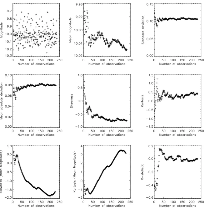
3.3 Statistical indices applied to a Cepheid type star as a function of time. The
indices are the same as in Fig. (3.2). . . 35
3.4 Statistical indices applied to aδ-Scuti type star as a function of time. The indices are the same as in Fig. (3.2). . . 36
3.5 Statistical indices applied to an eclipsing binary as a function of time. The indices are the same as in Fig. (3.2). . . 37
3.6 Statistical indices applied to an RR Lyrae type star as a function of time. The indices are the same as in Fig. (3.2). . . 38
3.7 Statistical indices applied to the light curve of a star with unknown variability as a function of time. The indices are the same as in Fig. (3.2). . . 39
4.1 Left panel: Details of the WFCAM focal plane. The four detectors are shown in their respective position relative to each other. Detector 1 shows the channel layouts. Right panel: The broad band filters used in WFCAM. We used only the JHK filters in our survey. . . 42
4.2 Left panel: Field distortion. Right panel: Differential non-linear distortion. . . . 43
4.3 Left panel: Diagram showing how the crosstalks appear in different quadrants. The crosstalk pattern rotates because the readout amplifier for each quadrant is located on a different edge of the detector, as shown by the red lines. Right panel: An example of crosstalk detected in one of our images. Whenever there is a saturated star, a crosstalk pattern will be present. . . 44
4.4 This figure shows how the dark frames, for all detectors, are dominated by the reset anomaly. . . 44
4.5 Left panel: Difference between two dark frames taken in order to show the decurtaining effect. Right panel: Dark frames with decurtaining solved. . . 45
4.6 This figure shows an example of persistent images in the WFCAM. . . 45
4.7 This figure shows an example of the flatfield correction. . . 46
4.8 WFCAM layout and reading scheme used to observe the ONC. . . 47
4.9 DADJHK - layout of the table containing all the photometric information. . . 48
4.10 (Mean Magnitude - Magnitude) versus Magnitude for the filter J, fourteenth night, for all the CCDs and areas. The panels are distributed in the same layout shown in Fig. (4.8). . . 50
4.11 Same as Fig. (4.10) but for the eighteenth night. . . 51
4.12 Light curves, Mean magnitude curves and phased light curves for three eclipsing binary candidates. . . 55
4.13 Light curves, Mean magnitude curves and phased light curves for three eclipsing binary candidates. . . 56
4.14 We present here the light curves, phased light curves, skewness and kurtosis curves (of the mean magnitudes) for the stars that presented rotation or pulsation. . . . 58
4.15 Same as in Fig. (4.14). . . 59
4.16 Same as in Fig. (4.14). . . 60
4.18 Same as in Fig. (4.14). . . 62
4.19 Same as in Fig. (4.14). . . 63
4.20 Same as in Fig. (4.14). . . 64
4.21 Same as in Fig. (4.14). . . 65
4.22 We show here examples of interesting light curves present in our sample. . . 66
5.1 The Great Cygnus Rift in Hα, image taken from Schneider et al. (2006). . . 68
5.2 The Great Cygnus Rift, extinction map taken from Schneider et al. (2006). The white circles represent the radio continuum sources detected by Downes & Rinehart (1966). . . 69
5.3 Cygnus OB2 star density map. The left panel shows the 2MASS data while the right panel shows the DSS red plates data. The image was taken from Kn¨odlseder (2000). . . 69
5.4 DADJHK and COORDS, layout of the tables containing all the astrometric and photometric information. . . 73
5.5 WFCAM layout and reading scheme . . . 74
5.6 The infrared sources revealed in our survey are displayed in this figure as filled circles. The sources are labeled using IDs found in the literature. The arrows in the bottom of the image represent the cometary globules we have found in our survey, the size of the arrow bodies correspond to the size measured from the head to the tail of the globule. . . 75
5.7 Cometary globules CG203446+411446 (panel a), CG203453+405320 and CG203442-+405115 (left and right on panel b) and CG203318+405911 (panel c). . . 76
5.8 Cometary globules CG203410+410700 (bottom) and CG203413+410813 (top). Both globules are associated with red stars in their heads. . . 77
5.9 Center region of the Cygnus OB2 association. The first cluster proposed by Bica, Bonatto & Dutra (2003) corresponds to the concentration of blue stars in the bottom-center of the figure. The second cluster corresponds to the top-center concentration. The very bright blue stars in the center, which are members of the association, were not taken into account by the authors. . . 78
5.10 IRAS 20321+4112 . . . 79
5.11 IRAS 20327+4120 . . . 80
5.12 IRAS 20332+4124 . . . 81
5.13 The IRAS 20333+4127 source. . . 82
5.14 JHK composite color of DR18. . . 83
5.15 Composite color image of the IRAS 20304+4059 infrared source. . . 84
5.16 Central area close up of the previous image. The red double object is associated to the IRAS source. . . 85
List of Tables
2.1 Pre-main sequence binaries with angular separation between 0.15′′
and 1.5′′
, outside the 60′′
exclusion zone aroundθ1 Ori C. . . 14
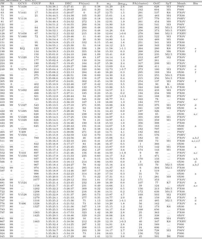
2.2 Other binaries with angular separations <1.5′′ toward the ONC. . . . 15
3.1 Statistical index values for all the variable stars in the test sample. . . 33
4.1 Observation log for the Orion Nebula. . . 47
4.2 Six candidates to be eclipsing binaries in M42 . . . 53
4.3 Objects candidate to be variable, selected through the study of statistical indices 57 4.4 Some objects presenting interesting light curves, identified with the procedures developed in the present work . . . 57
5.1 Cygnus OB2 properties, following Kn¨odlseder (2000) . . . 70
5.2 Observation dates of the Cygnus OB2 survey. . . 71
5.3 Cometary globule ID, coordinates, position angle and assumed size. . . 76
Resumo
Com o intuito de aumentar nosso conhecimento sobre estrelas jovens, realizamos trˆes levanta-mentos de larga escala, em duas regi˜oes de forma¸c˜ao estelar, a Nebulosa de ´Orion e a associa¸c˜ao de estrelas OB conhecida como Cygnus OB2.
O primeiro levantamento foi feito com a “Advanced Camera for Surveys - ACS” a bordo do telesc´opio espacial Hubble. Utilizamos um filtro estreito, centrado no comprimento de onda da linha Hα, para mapear a regi˜ao ao redor do centro da Nebulosa de ´Orion. Nosso principal objetivo ´e utilizar a alta resolu¸c˜ao da ACS (0′′.
05 por pixel) para detectar novos sistemas bin´arios visuais. Estabelecemos limites para a separa¸c˜ao entre as componentes dos sistemas bin´arios (0′′.
15 at´e 1′′.
5) utilizando testes de completeza da amostra e testes de probabilidade de proje¸c˜ao na linha de visada. Ap´os um minucioso estudo de cada sistema detectado em nossa amostra, conseguimos atingir nosso objetivo e observamos ind´ıcios claros da evolu¸c˜ao dinˆamica desses sistemas bin´arios na Nebulosa de ´Orion. Descobrimos 55 novos sistemas bin´arios visuais em uma amostra de 72 sistemas bin´arios e 3 sistemas triplos. Determinamos uma frequˆencia de bin´arias de (8.8±1.1)% na Nebulosa de ´Orion, um valor 1.5 vezes menor do que para o campo estelar e 2.2 vezes menor do que em associa¸c˜oes T. Esse j´a era um fato conhecido, mas baseado em estat´ısticas de poucos n´umeros, ao contr´ario dos nossos resultados, que foram obtidos com a utiliza¸c˜ao de uma amostra estat´ıstica mais significante. A raz˜ao entre o n´umero de sistemas com separa¸c˜ao grande e pequena aumenta significativamente a partir de 460′′
do centro do aglomerado, que ´e tomado como a estrelaθ1 Ori C. Esse fato, segundo nossa an´alise, ´e um ind´ıcio da evolu¸c˜ao dinˆamica do aglomerado, que acontece atrav´es da destrui¸c˜ao dos sistemas bin´arios com grandes separa¸c˜oes, ap´os algumas passagens pelo po¸co de potencial gravitacional do centro do aglomerado. Um sub-produto da nossa an´alise ´e a detec¸c˜ao de candidatos a objetos sub-estelares (an˜as marrons). Determinamos a natureza dupla do objeto COUP1061, classificado na literatura como uma an˜a marrom. Essa descoberta implica que o objeto COUP1061 ´e um sistema bin´ario composto por duas an˜as marrons, separados por aproximadamente 100 unidades astronˆomicas.
Os demais levantamentos foram feitos com a “Wide Field Camera” do “United Kingdom Infrared Telescope”. Observamos a Nebulosa de ´Orion e Cygnus OB2, na regi˜ao do infravermelho pr´oximo, nas bandas J, H e K. O objetivo desses levantamentos fotom´etricos ´e determinar a popula¸c˜ao de estrelas vari´aveis dessas regi˜oes de forma¸c˜ao estelar. Atrav´es da utiliza¸c˜ao de ´ındices estat´ısticos, as estrelas vari´aveis podem ser classificadas em seus diferentes grupos. Por se tratarem de levantamentos fotom´etricos de ´areas grandes, desenvolvemos rotinas especiais para lidar com os cat´alogos, compostos por dezenas e algumas vezes centenas de milhares de objetos.
necess´ario at´e se obter um conjunto de dados que pode ser utilizado para a busca de estrelas vari´aveis. Atrav´es da aplica¸c˜ao de ´ındices estat´ısticos conseguimos descobrir novas candidatas a bin´arias eclipsantes e estrelas com variabilidade causada por pulsa¸c˜oes ou por rota¸c˜ao. Um longo processo de an´alise ´e ainda necess´ario para exaurir a enorme quantidade de informa¸c˜ao presente nesse levantamento.
Abstract
In the attempt of increasing our knowledge about young stars, we performed three large scale surveys of two star forming regions, namely the Orion Nebula and the young OB association known as Cygnus OB2.
The first survey was made with the Advanced Camera for Surveys (ACS) onboard the Hubble Space Telescope. We used a narrow band filter, centered in the wavelength of the Hα line, to map the region around the center of the Orion Nebula Cluster. Our main goal is to use the high resolution of the ACS (0.′′
05 per pixel) to detect new visual binaries. We set the separation limit between the components of the system (0′′.
15 to 1.′′
5) using completeness tests and the probability of chance alignment. After a minute analysis of each system detected in our sample, we reached our goal and also observed clear evidence of the dynamical evolution of these systems in the Orion Nebula Cluster. We discovered 55 new visual binary systems within a total of 72 binaries and 3 triple systems. We determined a binary frequency of (8.8±1.1)% for the Orion Nebula Cluster, which is 1.5 times smaller than the frequency for the field and 2.2 times smaller than for the loose T associations. This was an already known fact but was based on small number statistics, while our results are based on more significant numbers. The ratio between wide and close binaries has a significant increase at 460′′
from the center of the cluster, assumed to be the star θ1 Ori C. Our analysis indicates that this is clear evidence of the dynamical evolution of the Orion Nebula Cluster, which happens through the destruction of wide binaries, after few passages through the cluster’s potential well. A byproduct of our survey is the detection of substellar candidates. We determined the double nature of the object known as COUP1061, which is classified in the literature as a brown dwarf. This finding implies that COUP1061 is a binary system where both components are brown dwarfs, separated by ∼100 AU.
In order to perform the second and third surveys we made use of the Wide Field Camera of the United Kingdom Infrared Telescope. We observed the Orion Nebula and Cygnus OB2 with near infrared filters, JHK. Our objective with these photometric surveys is to determine the population of variable stars in these star forming regions. Using statistical indices we can separate and classify the variable stars into different groups. Because these photometric surveys cover large areas in the sky we developed special routines to deal with the catalogs, which are composed of thousands and sometimes hundreds of thousands of objects.
Chapter 1
Introduction
Star formation is nowadays one of the most important branches in astronomy. It all started with the first observation of late-type low mass stars in the Taurus-Auriga region by Joy (1945). Later, these stars were proposed to be young stars by Ambartsumian (1957) and they were labeled T Tauri stars, after the object thought to be the prototype of young solar mass stars. Herbig (1960) observed the intermediate mass relatives of T Tauri stars, the Herbig Ae/Be stars. Since these pioneer works we have seen an incredible growth of observations, both in quantity and quality, which supported the establishment of different models of formation, evolution and structure of stars. We study these young stellar systems in the hope that they will give us hints about the history of our own Solar System. We try to understand how stars and planets form so that we can comprehend how the Earth, and other planets in the Solar System, formed when the Sun was only a few million years old.
One of the things we have learned, during the study of young stars, is that most of them are formed in multiple systems (e.g. Leinert et al., 1993; Mathieu, 1994; Duchˆene, 1999; Bodenheimer et al., 2000; Patience et al., 2002; Kroupa & Bouvier, 2003; Duchˆene et al., 2004; Haisch et al., 2004). If that is true then why is the Sun a single star? A multiple system can be disrupted by different mechanisms such as the fast decay of small-N systems (Sterzik & Durisen, 1998; Reipurth & Clarke, 2001; Durisen, Sterzik & Pickett, 2001; Hubber & Whitworth, 2005; Goodwin & Kroupa, 2005; Umbreit et al., 2005) and the dynamical destruction caused by multiple interac-tions in clustered environment (Kroupa, 1995a,b; Kroupa et al., 2003). The former mechanism acts at the beginning of star formation, while the molecular cloud core ends its collapse. Nonhierarchical systems with N>3 decay into single objects, binaries and hierarchical multiples. The latter acts during the whole life of the cluster. It consists of the interaction of multiple systems with the cluster’s potential well and with the crowded environment that surrounds the object. This interaction will disrupt multiple systems that are loosely bound. Some models also predict that environmental influences, such as the molecular cores’ temperature, could be important to define the initial binary fraction (Durisen & Sterzik, 1994; Sterzik, Durisen & Zinnecker, 2003).
of stars, are still unknown. Recently, Stassun et al. (2008) reported the discovery of a pair of “stellar twins” in a binary system. Each star has a mass of 0.41±0.01 M⊙, identical to 2%.
What makes the pair so special is the fact that although they are similar in mass, they have temperatures differing in ∼10% and luminosities by ∼50%, with high confidence levels. This binary system, with very similar components, though not identical as claimed by the authors, can give us hints about the influence that multiplicity can exert during the formation of stars.
Multiple systems play an important role in astronomy. They are very important for the calibration of evolutionary models and it is not much to say that the spectroscopic eclipsing binaries act in astronomy as “weights and rulers”. These systems, in particular, can give us very precise (.1%) absolute parameters (mass, radius, ratio of temperatures, etc) which can be used as constraints to theoretical models. Although multiple systems seem to be very common at the early stages of star formation, only 22 pre-main sequence stars have parameters measured through the use of dynamical techniques (Mathieu et al., 2007; Stassun et al., 2008). In order to discover more eclipsing binaries it is necessary to perform accurate and comprehensive surveys with long time-line bases.
Since the beginning of the study of young stars it became clear that they are extremely variable objects. In fact, photometric variability was one of the criteria used to classify them. Young stars present photometric and spectroscopic variability in all wavelengths, from radio to X-rays. Some of the variability is caused by the circumstellar material in different ways. Circumstellar material can cause variable extinction when it crosses our line of sight toward the object, causing sudden drops of brightness. The process of accretion, through which the star increases its mass, can still be active, causing variability in brightness. In young T Tauri stars the convection zone in their interior creates magnetic fields strong enough to produce large scale cool spots in the photosphere, which along with the star’s rotation produce a periodic modulation in the light curve. Flares in young stars, similar to solar flares, can also produce irregular photometric variability. The processes of accretion and ejection of matter can also change the line profile of many atomic species present in the photosphere of the star, giving birth to the spectroscopic variability in young stars (e.g. Guimar˜aes et al., 2006). Pulsation was also observed in young stars (e.g. Kurtz & Marang, 1995) situated at the instability strip of the HR diagram.
the Sloan optical bands (u’, g’, r’, i’, z’), the All Sky Automated Survey (ASAS, Pojmanski, 1997) in the optical V and I bands, the UKIRT Infrared Deep Sky Survey (UKIDSS) considered to be the successor to 2MASS, just to cite a few of them.
We are involved in the Variable Young Stars Optical Survey (VYSOS), which intends to continuously monitor stellar objects in star forming regions located in the Galactic plane and also to find new young objects in the same star forming regions. It was part of my project to work with the data collected by these telescopes.
The project consists of 2 small telescopes (the diameter of the main mirror is 41 cm), one installed in the northern hemisphere, at the Mauna Loa Observatory – Hawaii – USA, and the other in the southern, at Cerro Murphy – Chile.
Each telescope will be equipped with a set of Sloan filters (Fukugita et al., 1996) and an SBIG CCD, which has a dimension of 4096×2048 pixels and a pixel scale of 0′′.
77. Such a combination of pixel scale and dimension will produce a field of view of 27′
×40′
.
The northern telescope has been facing some mechanical and optical problems. In July 2006 I was at the Institute for Astronomy (IfA) in Hawaii, as part of my PhD program, when a major problem with the optical system was detected. The first problem was detected during the process of collimation. The optical system lacked one degree of freedom necessary to align the optical beam. This problem was reported to the engineers who built the system and some solutions were proposed by them. After trying different approaches we concluded that the missing degree of freedom was really necessary and the problem could not be solved without making a new base for the plain mirror, responsible for sending the optical beam straight to the camera. The difficulties in the process of alignment and collimation made us check the whole optical design and other problems were detected by Dr. Josh Walawender, a postdoc at IfA at that time. After calculations and studies of the optical system the conclusion was that it did not work, except in the optical axis. The set of optical lenses used to focus the beam leaving the tertiary mirror did not posses the necessary quality. Thus, due to construction and optical problems, the telescope was redesigned and many parts of it were rebuilt.
Formerly, the telescope was a modification of the Newtonian design. After being redesigned it was built as a Newtonian telescope. Such a modification brought some advantages, for example it decreased the number of mirrors and lenses used. The collimation and alignment were done easily this time. However, some issues remained, dealing mainly with the tracking system. We were not able to track during long exposures. Also, the telescope showed itself to be extremely sensible to vibrations of the dome. This problem was caused by the fact that there is not a separated pier for the telescope and all dome vibrations (caused by wind) were transmitted to the telescope through the floor. The floor where the telescope is fixed also presented some problems because it was not flat enough. The steel plates that should sustain all the weight of the telescope showed some signs of bending. A new mechanical problem was also found, caused by the 6.8 magnitude earthquake that stroke Hawaii on October 2006. The earthquake caused the telescope to bounce and the aluminum wheel responsible for the right ascension movement was slightly indented.
month but it is not working yet.
Thus, because our main project was delayed, we decided to study binary stars and variable stars from a different point of view. We will focus our attention in specific star forming regions, in order to build a comprehensive database, covering long periods, usually hundreds of days. Instead of looking at the whole sky, we will look at specific regions for a long time interval.
In our attempt to better understand multiple young stars, we report here the performance of an imaging survey using the Advanced Camera for Surveys, onboard the Hubble Space Telescope, of the well studied Orion Nebula. The main objective of this survey is to find new visual binaries in a wide region around the Orion Nebula Cluster. Previous studies have shown that the binary frequency of the Orion Nebula Cluster is lower than the binary frequency of the Galactic field. Does this fact have something to do with the dynamical evolution of the cluster? Can we distinguish between the two mechanisms responsible for the dynamical evolution of the binary properties? We will try to answer these questions in Chapter 2.
Our second incursion in the star formation domain is related to two near infrared large scale surveys of two different star forming regions. Our main goal is to unveil the young variable population of the Orion Nebula and of the young OB association Cygnus OB2. For this task we used the Wide Field Camera of the United Kingdom Infrared Telescope, the most capable infrared imaging survey instrument in the world, currently installed at the summit of the Mauna Kea Observatory. We will present in Chapter 3 some statistical techniques that can be used to characterize the variable star population in these fields. Light curves from the ASAS were used as tests in order to better understand the behavior of these statistical indices.
In Chapter 4 we will present the observations, procedures and results of the survey conducted in the Orion Nebula. We have built a database using 98 nights, from 101 observed nights covering 178 days, which is so far the longest infrared survey of the Orion Nebula. Many interesting variable objects were found after we applied the statistical indices to the database.
Cygnus OB2 will be analyzed in Chapter 5. It is a giant OB association, which was even considered to be a young globular cluster, given the number of O type stars associated to it (∼100 stars). Cygnus OB2 is situated in the Cygnus X star forming region, behind the Great Cygnus Rift. When we look in that direction of the sky, we are looking through the Local Spiral Arm and the Perseus Arm and, hence, we can see many star forming regions projected in the same area of the sky. A better analysis of its low and intermediate mass content is necessary in order to put constraints to its total mass and extent. We observed the center of this OB association during 112 nights, covering an interval of 217 days, but given the huge amount of data we were not able to construct the final database yet. However, four nights were used to construct a preliminary catalog, which we used to study the properties of this interesting star forming region. It is the richest infrared survey made for this association and given the attained angular resolution we will be able to double the number of objects associated to it.
Chapter 2
Visual Binaries in the Orion Nebula Cluster
2.1
Introduction
The Orion Nebula Cluster (ONC) is responsible for the ionization of the H II region know as the Orion Nebula (M42 + M43 = NGC 1976), one of the most studied regions in the sky. The ONC calls such attention because it is the nearest giant star forming region (∼450 pc). Its most massive stars, know as the Trapezium stars, are located in its center. They were thought to be a distinct entity (e.g. Herbig & Terndrup, 1986) but it has been argued that they are actually the core of the ONC (Hillenbrand & Hartmann, 1998).
The ONC is not only the nearest site of high-mass star formation but is also very young, with age∼1 Myr. Its youth is supported by:
• the stars located above the ZAMS (Zero Age Main Sequence) (Herbig & Terndrup, 1986; Prosser et al., 1994);
• the photometric variability of more than 50% of its stars (Jones & Walker, 1988; Choi & Herbst, 1996);
• the existence of optical emission line spectra (Herbig & Bell, 1988, and references therein); • the high polarization;
• the infrared excesses;
• the proplyds pointing towardθ1 Ori C (the most massive of the Trapezium stars).
The ONC has been studied in all wavelengths, from radio to X-rays. Since it is one of the most studied regions in the sky, a full review would be beyond the purpose of this work. We will focus our attention on the orbital evolution of its multiple systems.
An intriguing result of the study of the formation and evolution of binary systems is that binaries are more common (by a factor of 2) in T Tauri associations than in the field (e.g. Reipurth & Zinnecker, 1993; Simon et al., 1995; Duchˆene, 1999; Ratzka, K¨ohler & Leinert, 2005). A more intriguing result is that the ONC has a binary frequency lower than T Tauri associations and the field (e.g. Prosser et al., 1994; Padgett, Strom & Ghez, 1997; Petr et al., 1998; Simon, Close & Beck, 1999; K¨ohler et al., 2006).
The study of binary properties is marked by the detailed work with field binaries made by Duquennoy & Mayor (1991, hereafter DM91). The properties of the binary field population serve as a reference to the work on younger populations. But can we trust the binary field population? How is it formed? Does the field population come from a mix of other cluster populations (e.g. loose T associations, OB associations, open clusters and so forth)?
In the recent literature there are two main models for the evolution of binary properties: 1) fast dynamical decay of small-N systems within cluster cores (e.g. Reipurth & Clarke, 2001; Sterzik & Durisen, 1998, 2003; Durisen, Sterzik & Pickett, 2001; Hubber & Whitworth, 2005; Goodwin & Kroupa, 2005; Umbreit et al., 2005) and 2) dynamical destruction due to multiple interactions in a clustered environment (e.g. Kroupa, 1995a,b; Kroupa et al., 2003).
The first mechanism acts in the initial stages of star formation, during the Class 0 phase, while the second mechanism needs more time to act and does so for a longer time. We can thus say that the fast decay mechanism acts on a small scale (the scale of the multiple system) while the dynamical destruction mechanism acts on a larger scale (the scale of the whole cluster). We will call them fast decay mechanism (FDM) and dynamical destruction mechanism (DDM).
Assume we have stars forming in a cloud. During the collapse of the cores many multiple systems are formed. The FDM will act on these multiple Class 0 systems in a way that the less massive components will be ejected and the resultant binaries will have their semimajor axis decreased.
The DDM will act in all the systems during their whole lives within the cluster. In order to help us understand how this works we will divide the binary systems into three classes.
1. the wide, or soft, binaries; 2. the dynamically active binaries; 3. the tight, or hard, binaries.
The wide binaries have orbital velocities much smaller than the velocity dispersion of the cluster. The DDM will disrupt these systems and thus populate the field with single stars. The hard binaries, on the contrary, have an orbital velocity much greater than the velocity dispersion. These binaries will release energy to the cluster, becoming harder.
These facts lead Heggie (1975) and Hills (1975) to propose the following law: soft binaries soften and hard binaries harden.
An important point to note, coming from the computational simulations, is that dynamical interactions cannot form a significant number of binaries from an initially single star population (Goodwin et al., 2007).
Two points of view come into shock at this present time. Goodwin & Kroupa (2005) argue that almost all stars are formed in multiple systems, meaning that the initial binary fraction is close to unity. The later low binary fraction among M dwarfs would then be caused by the preferential destruction of these low mass systems. They are the first ones to be disrupted by both mechanisms. On the other hand, Lada (2006) argues that because most M dwarfs are single and most stars are M dwarfs, then most stars form as single stars.
K¨ohler et al. (2006) suggest that the initial binary frequency in the ONC was lower than in Taurus-Auriga. This fact suggests that the binary formation rate is influenced by environmental conditions. Their results do not agree with the mechanisms described by Goodwin & Kroupa (2005).
The statistics of binarity for the ONC were poor and concentrated on regions around the Trapezium stars. Such an important statement should be based on more solid grounds. We will show here, using significant numbers, that the ONC indeed has a lower binary fraction than the T Tauri associations and the field, as reported previously in literature.
We present here a study of the ONC using the Advanced Camera for Surveys (ACS) onboard the Hubble Space Telescope (HST). Our major goal is to study the binary frequency of the ONC, focusing on the outskirts of the cluster and excluding the inner region around θ1 Ori C. The results presented here were published in the Astronomical Journal, see Reipurth et al. (2007).
2.2
Observation and Catalogs
During program GO-9825, 26 fields were observed with the F658N filter (Hα+N[II]) and an exposure time of 500 seconds per pointing. These 26 fields when combined yield a mosaic image that covers an area of 415 arcmin2 with a very high angular resolution (0′′.05 per pixel). Further
details of the observations are described in Bally et al. (2006) and a schematic figure showing the disposition of the observed areas is shown in Figure (2.1).
Due to the high stellar density in the Trapezium region we excluded a circular region with radius 60′′
centered in θ1 Ori C, as can be seen in Fig. (2.1). We will not take this region into account in our work. We focus our attention on a larger area around the Trapezium, where we are able to probe the low mass stellar population.
We tested an automatic procedure to detect the stellar sources but it did not yield satisfactory results. The routines were written in IDL (Iteractive Data Language) and made use of the package IDLASTRO, which is a library with many routines written specifically to deal with astronomical issues.
Figure 2.1: Distribution of the visual binaries, with different separations, in the observed region. The grey solid circle, with a radius of 60′′ and centered inθ1 Ori C, is called the exclusion zone. We did not consider, in our
analysis, any star inside this zone. Single stars are plotted as asterisks and binaries (triples included) are plotted as black filled circles.
The roundness parameter is related to the geometric form of the object being searched, it is a 2-dimensional vector (between−1 and 1, the default values) and should only be changed if the objects are elongated. Since we have many saturated objects in our images this parameter was of not much use when applied to these cases and in fact introduced many false detections.
Thesharpnessparameter relates to the kind of statistical distribution followed by the objects. It is also a 2-dimensional vector where the default values are 0.2 and 1.0. These values should only be changed in case the objects’ point spread function is different from a Gaussian. As in the case of the roundness limit, the sharpness limit was not of much help while dealing with saturated objects and high background brightness.
The hminparameter is the threshold intensity for the point source. Its value should be 3 or 4σ above the background noise. We have very faint objects in our sample, thus we cannot put the threshold limit too high. However, setting this limit to a low value would also cause a very high number of detections, given the high background brightness variability. This parameter became our biggest problem while trying to use an automatic detection procedure.
We tested this automatic procedure many times, with different sets of values for the input parameters, but the output was far from useful. The procedure always returned several thou-sands of detections per image. Because of this we decided to search the image by eye, individually. We had to take some care while checking the stellar sources by eye because some images overlap, as can be seen in Fig (2.1). All the overlapping areas were carefully inspected and the stellar sources detected in more than one image were catalogued and counted only once. In the end we detected 1 051 stellar sources in the whole area.
The coordinates for each object were obtained using two routines, also written in IDL. The first one was responsible for obtaining the pixel coordinates of the stellar sources, through the use of a 2-dimensional Gaussian function. The center of the 2D-Gaussian was taken as the center of the stellar source. The pixel coordinates were then transformed to celestial coordinates with the IDLASTRO sub-routine called xy2ad.pro.
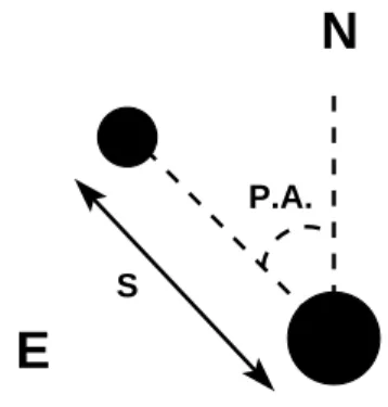
Once the stellar sources were catalogued we were able to go to the next step, selection of the multiple systems. Visual binaries have two important parameters, the position angle (PA) and the separation (S) between the pair. The position angle measures the angle between the primary and secondary and it is counted from North to East (counterclockwise), using the primary as reference. Figure (2.2) exemplifies the position angle and separation between two stars in a binary system.
N
P.A.
E
SFigure 2.2: Definition of the position angle (PA) and separation (S) between primary and secondary in a binary system.
To calculate the position angle we used an IDLASTRO subroutine called posang.pro. The separation between the stars was obtained in two distinct ways. The first method applies the IDLASTRO sub-routine gcirc.pro, which calculates rigorous arc distances in spheres. In the second method we used the pixel coordinates to obtain the distance between the objects in the plane of the image, discarding any deformation caused by the sky projection onto the plane of the CCD. Both methods yielded similar results, which can be explained by the fact that the separations are too small to be influenced by the projection of the celestial sphere onto the plane of the CCD, and also because the observed region is close to the equator, where the field deformation is less pronounced. Because some binaries have a very small separation (<0′′.
2.3
Membership of the ONC
We used 4 criteria to establish whether a star in our sample belongs to the ONC:
1. it has proper motion given by the Jones & Walker (1988, from now on, referred to as JW) catalogue and the membership probability is ≥93%;
2. it is listed as an ONC member by the X-ray survey performed by the Chandra satellite (COUP project – (Getman et al., 2005));
3. it presents irregular variability as listed by the GCVS (General Catalogue of Variable Stars);
4. it has Hα emission (detected in our unpublished catalogue).
A star does not need to obey all the criteria at the same time, it is sufficient to present one of them to be classified as a member of the ONC. From 1 051 stars in our sample, 655 are listed in the JW catalogue and 596 have a membership probability≥93%. We want to point out that most of our binaries are not resolved in the JW survey, given it was made with photographic I-band plates. This fact implies that the proper motions can be affected by changes in the brightness of the companion stars. We observed such variations in our sample. One of our binaries is located on the edge of two images which overlap themselves. Since the observations were made in different epochs we were able to detect a brightness variation in the system. Such variation can change the photocenter of the pair (in an unresolved image, like the photographic plates used by JW) and thus lead to a wrong proper motion. We also would like to point out that some stars with 0% membership probability showed signs of youth, which is good evidence of its association with the ONC. Hence, we concluded that the proper motion information is useful to support the membership of a system, but such information should not be used to exclude membership. Information about the youth of the system can be gathered from other sources, like X-ray emission, Hα emission and photometric variability. That is the reason why we used the COUP catalogue (X-ray), the GCVS (variability) and the unpublished Hα catalogue. Not all young stars present Hαemission, but we assume that a star in the Orion region that presents such emission line is young. From the 1 373 ONC members in the COUP catalogue, we found that 658 are present in our sample. We found 196 variable stars in our sample and 99 stars presented Hα emission.
the discovery paper in case the binary was already known and the letters correspond to the references: a - Prosser et al. (1994); b - Padgett, Strom & Ghez (1997); c - Simon, Close & Beck (1999); d - K¨ohler et al. (2006); e - Getman et al. (2005); f - Lucas, Roche & Tamura (2005).
Table (2.2) lists binaries that were found in our sample but that were not used in our analysis. The reasons for not using these binaries are: three binaries have separation in the range 0′′.
11 and 0′′.
15, other three binaries are within the exclusion zone and have separations less than 0′′. 4 and seven binaries do not show any evidence of membership to ONC. The columns in Table (2.2) are the same as in Table (2.1) with one more column that characterizes the binaries as: 1 - binaries with angular separation< 0′′.
4 inside the exclusion zone; 2 - binaries with angular separation <0′′.
15 outside the exclusion zone and 3 - binaries with angular separation < 1′′. 5 outside the exclusion zone but with no evidence of ONC membership .
With the exception of the object JW 945, which is a Herbig Ae/Be star, all of the binaries in our sample consist of late-type stars, see Table (2.1). Figure (2.3 presents stamps for the 72 visual binaries, 3 visual triples and also the 3 visual binaries inside the exclusion zone.
2.4
Completeness
Since our major goal is to search for visual binaries in the ONC, we have to account for the contamination due to line-of-sight alignment. We must set an inferior and a superior separation limit for our search.
The inferior limit was determined based on the angular resolution obtained with the ACS (0.′′
05) and with a blind test. We selected 5 stars in our images that presented a good Gaussian profile. An IDL routine was written to copy this Gaussian profile and create artificial stars, which were then positioned beside real stars but with random separations, position angles and flux ratios. Seven sets of 25 images each were created. One example of the artificial binaries is shown in Fig (2.4).
The blind test consists of looking at each image in sequence during no more than 5 seconds. If the pair is visible and easily detected, we call it a positive target. If it is not possible to detect the pair within 5 seconds, we call it a negative target. Three of us (Bo Reipurth, Michael Connelley and I) did this test for each set of artificial binaries and the positive and negative targets were added. If one person counted a target as positive but the other two counted it as negative, the target was then counted as negative. Likewise, two positives and one negative was counted as one positive.
Figure (2.5) presents the results of this blind test. Our observed binaries are shown in the left panel. The right panel shows the detections found during the blind test, where filled circles indicate systems in which we could detect the companions and open circles represent those in which we were not able to. We can detect binary systems down to 0′′.
10, however, our sample will not be complete in this limit, as can be seen in Fig. (2.5). We have set our inferior limit to 0′′.
Figure 2.3: All binaries identified among the ONC members. Each stamp is 2′′wide, with north pointing up
Table 2.1: Pre-main sequence binaries with angular separation between 0.15′′and 1.5′′, outside the 60′′exclusion
zone aroundθ1 Ori C.
JW % GCVS COUP RA DEC PA(sys) S mI ∆mH α PA(cluster) OriC SpT Memb. Bin 39 99 V1438 ... 5:34:38.1 -5:27:41 21 0.38 14.29 2.6 246 628 M3 P00V 52 98 ... ... 5:34:40.8 -5:28:09 231 0.20 14.58 0.1 242 604 M5 P000 63 99 V1441 17 5:34:43.0 -5:20:07 0 0.27 12.75 1.5 291 537 K6 PX0V 71 99 ... 21 5:34:44.5 -5:24:38 105 0.20 15.61 1.4 261 483 M4 PX00 73 99 V1118 ... 5:34:44.7 -5:33:42 329 0.18 14.04 0.4 217 779 M1 P0HV 81 97 ... 28 5:34:46.4 -5:24:32 272 1.34 12.91 1.9 261 454 M0 PX0V 121 99 ... ... 5:34:51.2 -5:16:55 200 0.34 14.90 3.0 316 541 M3 P00V 124 99 ... 64 5:34:51.8 -5:21:39 200 0.48 13.94 0.0 286 382 M3.5 PX0V 127 99 ... 66 5:34:52.1 -5:24:43 254 0.48 14.28 0.6 258 373 M3.5 PXHV 128 97 V1458 67 5:34:52.2 -5:22:32 215 0.39 12.64 >0.6 278 366 M2.5 PXHV 135 99 V1460 72 5:34:52.7 -5:29:46 11 0.40 14.45 0.1 223 522 M3 PX0V 147 99 ... ... 5:34:54.4 -5:17:21 26 0.30 14.80 1.4 318 489 M5 P000 151 99 ... 95 5:34:54.8 -5:25:13 332 0.15 15.44 1.6 251 341 M3 PX00 152 99 ... 96 5:34:55.1 -5:25:30 51 0.18 14.12 2.5 248 343 M3 PX00 176 99 KQ 123 5:34:57.8 -5:23:53 336 1.28 11.58 >1.1 264 280 K8 PX0V e 190 99 ... 134 5:34:59.3 -5:23:33 355 0.56 15.33 0.3 268 256 M6 PX00 f 201 99 ... 150 5:35:01.0 -5:24:10 246 1.09 13.41 0.8 258 235 M2.5 PXH0 222 98 V1320 174 5:35:02.2 -5:29:10 89 1.07 14.14 1.4 212 407 M2 PX0V 223 99 ... 177 5:35:02.4 -5:20:47 130 0.34 13.64 1.3 307 261 ... PX00 224 99 ... 180 5:35:02.7 -5:19:45 164 0.27 15.38 2.4 317 299 M1 PX0V 235 0 ... 197 5:35:03.6 -5:29:27 346 0.54 13.69 0.4 208 411 ... PXHV d 248 99 V1274 214 5:35:04.4 -5:23:14 320 0.90 12.73 >3.7 273 180 M3 PX0V e ... ... ... 260 5:35:06.2 -5:22:13 284 0.40 16.20 0.3 295 169 M4 0X00 f 296 99 ... 275 5:35:06.6 -5:26:51 196 0.89 14.30 3.2 215 255 M4.5 PX00 296 99 ... 275 5:35:06.6 -5:26:52 158 0.27 14.30 0.4 215 256 M4.5 PX00 305 99 ... ... 5:35:07.6 -5:24:01 302 0.45 14.58 0.3 254 137 M3 P00V f 355 0 ... 402 5:35:10.9 -5:22:46 197 0.42 15.03 3.5 294 90 K: 0X00 370 99 ... 452 5:35:11.9 -5:19:26 122 0.73 13.86 3.5 344 246 K1.5 PX00 383 99 V1492 489 5:35:12.7 -5:16:14 280 0.19 14.57 2.1 353 433 M3 PX0V 392 99 ... 498 5:35:12.7 -5:27:11 185 0.23 15.21 0.2 194 234 M6 PX00 391 99 ... 501 5:35:12.8 -5:20:44 94 0.29 12.97 >3.3 341 168 M1 PX0V 399 99 ... 523 5:35:13.2 -5:22:21 345 0.22 16.77 0.1 322 78 ... PX00 a,c 410 99 ... ... 5:35:13.2 -5:36:18 167 1.19 16.00 1.3 184 777 ... P00V 406 99 V1327 543 5:35:13.5 -5:17:10 271 0.95 13.88 2.6 353 375 M1 PX0V d
... ... ... 562 5:35:13.6 -5:21:21 62 0.24 16.27 1.5 341 129 M3 0X00 a 422 99 V1495 566 5:35:13.7 -5:28:46 74 0.31 14.43 0.0 187 326 ... PX0V 436 0 ... 620 5:35:14.3 -5:22:04 238 0.32 16.97 1.0 338 85 ... 0X00 a,c 439 99 V1329 626 5:35:14.5 -5:17:25 150 0.30 14.97 0.1 355 359 M1 PX0V 439 99 V1329 626 5:35:14.5 -5:17:25 78 1.21 14.97 4.1 355 359 M1 PX0V 444 99 ... 651 5:35:14.6 -5:16:46 190 0.18 15.53 1.0 356 398 ... PX00 445 26 ... 645 5:35:14.7 -5:20:42 191 0.44 14.67 1.8 351 163 ... 0X00 a
... ... V1500 ... 5:35:14.9 -5:36:39 82 0.38 14.45 2.2 182 797 ... 000V 465 97 V409 ... 5:35:14.9 -5:38:06 271 0.43 14.71 4.1 182 883 ... P00V 498 99 V1504 ... 5:35:15.8 -5:32:59 122 0.70 13.81 0.2 181 576 ... P0HV 509 99 ... 789 5:35:16.2 -5:24:56 46 0.49 15.06 0.1 182 93 ... PX0V a,b,f 511 99 ... ... 5:35:16.3 -5:22:10 241 0.41 15.67 2.4 358 73 M1 PX00 a,c,e,f
... ... ... 822 5:35:16.8 -5:17:17 84 0.26 16.37 0.5 1 366 ... 0X00 551 99 ... 881 5:35:17.4 -5:25:45 265 0.14 13.87 0.0 174 142 M1 PX00 a 551 99 ... 881 5:35:17.4 -5:25:45 262 1.27 13.87 3.6 174 143 M1 PX00 552 99 V410 897 5:35:17.5 -5:21:46 156 0.46 14.50 >1.8 9 99 ... PX0V a,c 560 98 V1334 927 5:35:17.9 -5:15:33 235 0.60 14.17 3.2 3 471 ... PX0V 570 99 ... 937 5:35:17.9 -5:25:34 0 0.15 14.73 0.8 170 133 ... PX00 a,b 566 0 ... 939 5:35:18.0 -5:16:13 214 0.86 14.93 0.0 3 430 ... 0X00 d
... ... ... 967 5:35:18.4 -5:24:27 78 0.42 15.16 2.4 155 70 M2.5 0X00 a,b,f 592 99 ... 974 5:35:18.5 -5:18:21 285 0.61 14.37 4.0 6 304 M2.5 PX00 597 0 ... 994 5:35:18.8 -5:14:46 307 0.17 14.02 0.1 4 519 ... 0XHV
... ... ... 998 5:35:18.8 -5:22:23 314 0.20 17.54 0.3 31 70 ... 0X00 a ... ... ... 1061 5:35:20.0 -5:18:47 71 0.22 17.31 0.1 11 281 M9 0X00 638 99 ... 1077 5:35:20.0 -5:29:12 354 1.01 17.03 3.2 171 353 ... PX0V 681 99 V1524 ... 5:35:21.4 -5:23:45 232 1.09 16.39 0.9 107 77 K7 PX0V a 687 54 ... 1158 5:35:21.7 -5:21:47 231 0.49 14.66 2.1 39 124 ... 0X0V a,c 709 99 ... 1202 5:35:22.2 -5:26:37 309 0.22 12.92 0.5 156 213 M0.5 PX00 722 98 ... 1208 5:35:22.3 -5:33:56 216 0.36 14.51 0.2 172 639 M4.5 PX00 727 99 V1528 1233 5:35:22.8 -5:31:37 285 0.73 13.87 4.7 169 503 M2 PXHV 748 99 ... 1279 5:35:24.1 -5:21:33 277 0.35 14.77 2.0 46 159 M3 PX0V a 767 99 ... 1316 5:35:25.2 -5:15:36 75 1.13 13.89 >4.1 16 485 M2.5 PX0V d 776 99 V496 1328 5:35:25.4 -5:21:52 73 0.50 14.20 1.8 56 162 ... PX0V a 777 80 ... 1327 5:35:25.5 -5:21:36 347 1.19 15.15 1.2 52 173 K6 0X00 783 95 ... ... 5:35:25.5 -5:34:03 283 0.40 14.17 0.8 168 656 ... PX00 797 99 ... 1363 5:35:26.6 -5:17:53 323 1.42 16.30 2.8 25 363 ... PX00 ... ... ... 1425 5:35:29.5 -5:18:46 329 0.23 16.06 2.6 35 338 ... 0X0V 841 99 ... ... 5:35:30.0 -5:12:28 16 0.41 14.41 0.1 17 686 M4 P0HV 867 99 ... 1463 5:35:31.3 -5:18:56 212 0.29 12.19 >0.3 40 347 K8 PXHV 884 99 ... ... 5:35:32.4 -5:14:25 287 1.32 14.91 2.8 24 589 ... P000 893 99 ... ... 5:35:33.2 -5:14:11 208 0.15 14.07 0.0 24 606 ... P00V 906 99 ... ... 5:35:34.7 -5:34:38 293 1.39 14.17 2.7 158 728 M3 P00V 924 99 ... ... 5:35:36.5 -5:34:19 73 1.04 16.63 1.3 156 722 ... P000 945 99 ... ... 5:35:40.2 -5:17:29 46 1.41 12.51 3.6 45 501 B6 P000
P(Σ,Θ) = 1−e−πΣΘ2
(2.1)
Table 2.2: Other binaries with angular separations<1.5′′toward the ONC.
JW % GCVS COUP RA DEC PA SEP mI ∆mH α PA OriC SpT M Bin C 553 99 V1510 899 5:35:17.6 -5:22:57 113 0.36 12.41 1.4 34 31 K3.5 PX0V a 1 596 99 AF 986 5:35:18.7 -5:23:14 78 0.30 13.06 2.2 75 34 K3.5 PX0V 1 ... ... ... 1085 5:35:20.2 -5:23:09 104 0.21 ... 0.4 76 57 ... 0X00 1 182 48 ... 127 5:34:58.0 -5:29:41 77 0.11 16.56 0.2 216 467 ... 0X00 2 290 99 ... 266 5:35:06.4 -5:27:05 84 0.11 15.48 1.3 214 268 ... PX00 2 ... ... ... 1195 5:35:22.3 -5:18:09 227 0.11 15.67 0.8 15 326 ... 0X00 2 ... ... ... ... 5:34:19.5 -5:27:12 168 0.56 10.52 0.1 255 881 G5 3 58 0 ... ... 5:34:41.8 -5:34:30 282 1.43 16.13 2.2 218 844 ... 3 61 46 ... ... 5:34:42.7 -5:28:37 153 0.45 13.52 0.9 238 594 ... 3 ... ... ... ... 5:34:45.8 -5:30:58 324 0.46 ... 0.1 225 645 ... 3 ... ... ... ... 5:35:01.4 -5:24:13 292 0.28 ... 0.6 257 231 ... 3 ... ... ... ... 5:35:18.3 -5:24:39 96 0.67 16.72 2.2 160 81 ... 3 ... ... ... ... 5:35:30.0 -5:34:31 237 1.29 ... 0.3 163 699 ... 3
Figure 2.4: Examples of the artificial binaries, created using the profiles of real stars of our sample, in order to analyse our completeness.
1′′.
5. Because Correia et al. (2006) do not describe in detail the meaning of this equation, we decided to give more details about it in the following.
First, we need to know what is the probability of finding a companion to a primary star given a certain separation Θ. We can translate this to the following equation (P stands for primary and C for companion):
prob(P in field AND C within Θ) = prob(P in field)prob(C within Θ) (2.2)
The probability of the primary being in the field is 1, because we are using it as the central star. In order to calculate the probability of finding a companion within the given radius, we will use the Poisson distribution, because these are rare events and we have lots of trials. Using the Poisson distribution we have:
prob(C within Θ) =e−µ=e−πΘ2Σ
(2.3)
Figure 2.5: These two plots show the ∆m versusbinary separation in arcseconds. The observed binaries are shown in the left panel, where the dashed line indicates the 0′′.15 separation limit. The right panel shows the artificial binaries, created from real stars present in our images, with different separations, position angles and ∆m. In the right panel, filled circles indicate systems where we could detect the companions, while open circles represent those where we were not able to detect them.
Hence, the probability of finding a companion to a star, given a certain radius is:
prob(P in field AND C within Θ) =e−πΘ2Σ
(2.4)
Now that we know the probability of finding a companion, we only have to subtract 1 to find the probability of a companion being a line-of-sight contamination, which was given in Eq. (2.1).
To calculate the surface density we applied two distinct methods. The first method consists of counting the number of stars inside a circle of 30′′
radius centered on each star of our sample and dividing this number by the area of the circle. This way we obtain a local density of stars which are influenced by the subclusters in that specific area. The second method consists of defining large circular areas starting from the exclusion zone. Each annulus has width of 30′′
and the density was again obtained counting the stars inside each area and dividing by the area of the annulus. One problem with this method is the shape of our mosaic, which can be seen in Figure (2.1). Because we centered each annular area in θ1 Ori C, when the radius increases beyond 60′′
we start to have part of the annulus outside our surveyed area. We fixed this problem by calculating the area outside the mosaic, which means that the area used to calculate the density takes into account only the amount inside the mosaic. The first annulus has inner radius starting at 60′′
and outer radius at 90′′
. The second annulus starts at 90′′
and ends at 120′′
. The other areas continue with a step of 30′′
each with the last annulus having an outer radius of 1 020′′
. In the end we came to the conclusion that the correct procedure should be the first one because it was the only way to account for the subclustering observed in the Hα images.
The value of 1′′.
Figure 2.6: Left panel: surface density profile of the ONC members as a function of distance toθ1 Ori C. The exclusion zone is indicated by the dashed line. This profile was used as a guide to understand and localize the subclustering in the region studied. It was not used to obtain the probability of chance alignment. Right panel: probability that a star would have a companion as a line-of-sight association, obtained with Eq. (2.1). Presented here are all the 781 ONC members, squares for single stars and circles for binaries. One can see a subclustering around 180′′. We used the surface density obtained considering the number of stars inside an area of 30′′centered
in each star.
this separation these systems are still gravitationally bound) without compromising the overall contamination of false pairs. To obtain the number of false pairs we added up the probability of being a chance alignment of all the stars (781 members). We have 9 flase pairs in our sample, which means we have a contamination of 11% (9 false pairs among 781 members). Thus, the superior limit (1.′′
5) was chosen as the separation that minimizes the contamination by false pairs but still provides systems that are likely to be physically related.
The left panel of Fig. (2.6) shows the ONC density profile, calculated using the second method described above, while the right panel shows the probability of the companion being a line-of-sight association. In both panels it is possible to see a subclustering in the analyzed area. Since we are using a narrow band filter, which is extremely sensitive to the background brightness, we cannot be sure if the subclustering is real or not. It exists in our Hα images, however, there are many stars which were not detected in these images. This is another completeness problem in our sample and it is an unquantifiable one.
2.5
Results
2.5.1 Binary Fraction
With our range set to 0′′. 15 – 1′′.
5, we have 72 binaries and 3 triples, members of the ONC. If we correct this number for the contamination described previously and count 1 triple as 2 binaries we end up with 69 physical binaries. Such a number implies a binary fraction of (8.8±1.1)% in the interval 67.5 to 675 AU (0′′.
15 to 1′′.
5), where the error was estimated as 1σ based on Poisson statistics. If we count one triple as a single system we can calculate the multiplicity frequency, which gives us a value of (8.5±1.1)%, with errors estimated in the same previous way.
Analyzing the inner 40′′
×40′′
area of the Trapezium cluster, Petr et al. (1998) found four binaries in the separation range 0′′.
14 – 0′′.
In the same separation range we have 50 binaries leading us to a value of (6.4±0.9)%. The numbers agree inside the error bars, however one must remember that we do not analyse the inner zone of the Trapezium.
Reipurth & Zinnecker (1993) observed nearby T Tauri associations and found 38 binaries out of 238 stars in the range 150 – 1800 AU. The common range between our work and Reipurth & Zinnecker is 150 – 675 AU. We calculated the binary fraction (counting the three triples as six binaries) in this common range for both samples. The numbers are: (11.8±2.2)% for the nearby T Tauri associations and (5.3±0.8)% for ONC. These numbers lead us to conclude that the binary fraction in T Tauri associations is higher than in ONC by a factor of 2.2, in qualitative agreement with Petr et al. (1998).
2.5.2 Separation Distribution Function
The left panel of Figure (2.7) presents the separation distribution function in an angular scale, with bins 0′′.
1 wide. There is a clear decrease in the number of binaries with separations larger than 0′′.
5. The same distribution, but in a logarithmic scale, is presented in the right panel of the same figure, where we also plotted the binary contamination and the distribution of the field stars based on DM91. The contamination by line-of-sight pairs was calculated using Eq. (2.1), but with the separation parameter set to the separation of each pair, the probabilities were added up for each bin. This approach is meaningless for individual objects but it can be used to distribute the false binaries in each bin. For example, the total of the probabilities for all the systems in the last bin in the right panel of Fig. (2.7) is 68%. This means that out of the 9 false binaries in our sample, 6 are located in this bin. The bins with the larger separations have a larger number of false binaries, as expected. The errors are indicated by the straight lines and were calculated assuming a binomial distribution.
Using our whole range of separations we have a binary fraction of (8.8±1.1)%, while using data from DM91, in the same range of separations, we estimated a binary fraction of 13.7% and 12.4%, using a trapezoidal approximation and a linear interpolation, respectively. It was necessary to convert the periods given by DM91 to angular separations. Since the stars analyzed by DM91 are solar-like stars (F9-G6 V) we assumed a typical G2V spectral class and transformed the periods to separations. Hence, the field has a binary fraction 1.5 higher than ONC.
2.5.3 Wide versus Close Binaries
Is there a difference between the number of wide binaries and close binaries? Previous studies (e.g. K¨ohler et al., 2006) tried to find such difference without success. The dramatic change in the separation distribution function seen in the left panel of Fig. (2.7) lead us to choose this separation as a dividing point. Binaries with angular separation in the range 0′′.
15 ≤separation ≤0′′.
5 are called “close” and binaries with angular separation in the range 0′′.
5 < separation≤ 1′′.
5 are called “wide”.
To study the distribution of these systems as a function of separation to θ1 Ori C we build cumulative distributions like the ones shown in Fig (2.8). The left panel shows a simple cumulative distribution as a function of distance toθ1Ori C, created by adding up the close and wide binaries as the distance toθ1 Ori C increases, in steps of 1′′
Figure 2.7: The left panel shows the histogram of binary angular separations in steps of 0′′.1. The number of binaries in the innermost bin, with separations less than 0.′′1, is incomplete. We filled this bin with vertical
dotted lines. One can see the abrupt decrease in the number of binaries when the separation increases beyond 0′′.5. The right panel shows the logarithmic separation distribution function of the ONC binaries compared to the distribution of field binaries from Duquennoy & Mayor (1991) across the separation range from 0′′.15 to 1′′.5.
The dot-filled part of the histogram bins represents the contamination by line-of-sight pairs, obtained using Eq. (2.1). The bins representing large separations are the most contaminated ones, as expected. The vertical solid lines present in each bin represent the 1-σerrors calculated using a binomial distribution. The data from DM91 within our separation range are shown as two dashed crosses, while the Gaussian distribution they fit to their complete data set is represented by the dash-dotted line, which can be seen above the histogram. The top axis indicates separations in arcseconds at the distance of the ONC.
close binaries are not exclusive of the center regions and that we can detect wide binaries close to the center as probably as far from it. However the distributions are not the same.
The right panel in Fig. (2.8) shows a different situation. Here we have the ratio of wide to close binaries as a function of distance to θ1 Ori C. The cumulative distribution function was calculated in the following manner: the first point was calculated dividing the total number of wide binaries by the total number of close binaries with distances to θ1 Ori C, starting in the exclusion zone and going up to 30′′
from it (the exclusion zone is at 60′′
from θ1 Ori C, which means that the first step used stars with distances fromθ1 Ori C in the range 60′′
to 90′′
), the next step increased the distance in 1′′
and made the same calculation. In this way, as the curve moves away from θ1 Ori C it accounts for more and more binaries until it reaches the end of the distribution, where we have the mean ratio of wide-to-close binaries for the ONC. In the figure, the dashed lines indicate the 1σ errors and the dotted lines indicate the same ratio for the DM91 binaries, assuming a Gaussian fit (lower line), and the actual data points (upper line). The DM91 lines represent the ratio for field stars.
It is evident that there is a very pronounced and almost monotonic change in the ratio of wide-to-close binaries as one moves away from the core of the ONC until a distance of about 460′′, at which point the ratio becomes flat. It is also clear that the mean ratio of wide-to-close
binaries for the whole ONC is lower than DM91 values.