I
3d GIS modeling using ESRI´s CityEngine
A case study from the University Jaume I in
Castellon de la Plana Spain
Subtitle
II
3d GIS modeling using ESRI´s CityEngine
A case study from the University Jaume I in Castellón de la plana Spain
Dissertation supervised by PhD Michael Gould And co supervised by
PhD Joaquin Huerta PhD Marco Painho
III
Acknowledgments
IV
3d GIS modeling using ESRI´s CityEngine
A case study from the University Jaume I in Castellón de la plana Spain
ABSTRACT
V
Smíði LUK þrívíddar líkans
Ferilsathugun framkvæmd á háskólasvæði University Jaume I í Castellon
de la plana á Spáni
Útdráttur á Íslensku
VI
KEYWORDS
GIS Applications City Models 3d
VII
ACRONYMS
CAD – Gomputer-aided Design
CGA – Computer Generated Architecture
GIS – Geographical Information Systems / Sience MTL – Material Template Library
MTL – Material Template Library OBJ – Object File
UJI – Universidad Jaume I
VIII
INDEX OF THE TEXT
Table of Contents
3d GIS modeling using ESRI´s CityEngine ... II
Acknowledgments ... III
Smíði LUK þrívíddar líkans ... V
KEYWORDS... VI
ACRONYMS ... VII
1.
INTRODUCTION ... 1
2.
Theoretical Framework ... 3
6.1. Looking ahead ...4
2.1.1. Data structures and types ... 4
2.1.1. The multipatch ... 5
2.1. Mass 3d modeling ...5
2.2. Shape grammar ...6
3.
CityEngine ... 8
2.1. The user interface ... 9
4.
Methods ... 13
4.1. Setting up the projection ... 13
4.2. The base layer ... 14
4.2.1. Building the street network graph ... 17
4.2.2. Assigning the Modern Streets template to the graph ... 20
4.2.3. Creating a cga rule file for the LandscapeArea layer ... 26
4.2.4. Creating a cga rule file for the StreetPavement layer... 34
4.2.5. The double walking path and parking lot planter... 36
4.3. Indoor mapping ... 38
4.3.1. Data preparation ... 38
4.4.1. The outer shell ... 40
4.4.2. The interior ... 42
5.
Discussions ... 46
5.1.1. Strong points ... 46
5.1.2. Weak points ... 46
6.
Conclusion... 49
IX
Annex B ... 59
Annex C ... 77
Annex D ... 82
INDEX OF TABLES
X
INDEX OF FIGURES
Figure 1: An overview map of the UJI Campus. ... 2
Figure 2: Streets grown in CityEngine. ... 8
Figure 3: The default user interface of CityEngine... 9
Figure 4: The datasets used in the base layer. ... 14
Figure 5: The polygons after the cut operation ... 15
Figure 6: The 12 polygons that need to be cut ... 15
Figure 7: The street classification applied to the UJI Campus... 16
Figure 8: demostrating how vertices must be added where the pavement touches the streets. ... 17
Figure 9: Example of how the street network graph must fit tightly inside the LandscapeArea layer. ... 17
Figure 10: CityEngine generated roundabout. ... 18
Figure 11: The completed network graph. ... 19
Figure 12: Crosswalks over the major and minor streets at the UJI campus as seen in Google maps. ... 23
Figure 13: The major and minor road crosswalks after the new rules were assigned to them. ... 25
Figure 14: Screenshot of the attributes after categorisation in the inspector tab. ... 27
Figure 15: Grass texture. ... 28
Figure 16: Curb texture. ... 28
Figure 17: Gravel texture. ... 28
Figure 18: The tree obj model ... 29
Figure 19: A planter at the campus grounds. ... 30
Figure 20: The polygon representation of the planter. ... 31
Figure 21: The planter constructed in CityEngine. ... 33
Figure 22: The resulting planter after applying the planter rule to it. ... 34
Figure 23: the texture used for the Sidewalk and curb. ... 34
Figure 24: the texture used for the walking path. ... 34
Figure 25: the texture used for the streets. ... 34
Figure 26: The double zebra polygon with the texture assigned to it. ... 36
Figure 27: The double zebra seen in Google Earth. ... 36
Figure 28: A street wiew from the UJI campus after generating the rules. ... 37
Figure 29: Indoor spaces first floor... 39
Figure 30: Indoor spaces sub floor. ... 39
Figure 31: Indoor spaces ground floor ... 39
Figure 32: Indoor spaces second floor ... 39
Figure 33: Indoor spaces third floor ... 39
Figure 34: The sub floor shell. ... 39
Figure 35: The ground floor shell. ... 39
Figure 36: The first floor shell. ... 39
Figure 37: The second floor shell. ... 39
Figure 38: The Rectorate. ... 41
Figure 39: Model of the rectorate ... 42
1
1. INTRODUCTION
The field of GIS is currently undergoing a major shift in visualization technology. With the oncoming of ever more powerful computers the restrictions of the 2d mapping traditions no longer apply. Although the history of GIS and computer mapping systems date back to the 1960s (Coppock et. al., 1991), it is not until recently that digital maps have been elevated to 3d (Elwannas, 2011).
The first devices to commercially utilize 3d maps have been navigation devices such as handheld GPS systems, navigators for cars and airplanes, although not full 3d but usually defined as 2.5d.
The main driving force behind 3d development has been the computer gaming and animation industry and now we are witnessing the merging of those kinds of computer graphics with GIS. One of the biggest GIS software developer ESRI is currently taking a big step towards full 3d visualization by acquiring one of the leading companies in development of 3d urban modeling software Procedural. In 2008 Procedural released the software CityEngine for the creation of 3d cities in a quick and relatively simple manner using procedural modeling language. The program uses procedural modeling methods combined with shape and split grammars for generation of 3d content.
The goal ESRI has set itself is to make CityEngine a part of their ArcGIS family of applications. Jack Dangermond president of ESRI stated at the ESRI's 2011 International User Conference: “Many GIS problems can only be solved in 3D, particularly in the area of urban development, Procedural’s unique capabilities for generating high-quality 3D data,
using the same GIS data our users already have, makes them a perfect match for
Esri.” (Handrahan, 2011).
The main focus of this research paper is on testing the latest version of CityEngine published by ESRI in 2012 for 3d map making purely from a GIS perspective. The goal is firstly to look into CityEngine and see if it can in fact be used to generate 3d models of a “real city”. The dataset is a conventional 2d GIS data stored in an ESRI file geodatabase derived from a CAD architectural drawing of the area. It has been imported into a file geodatabase that is based on the local government template, for further information see (ArcGIS Resouces, 2013b).
2
brief experiment will also be conducted with indoor mapping using CityEngine to see if the software can be used for that purpose.
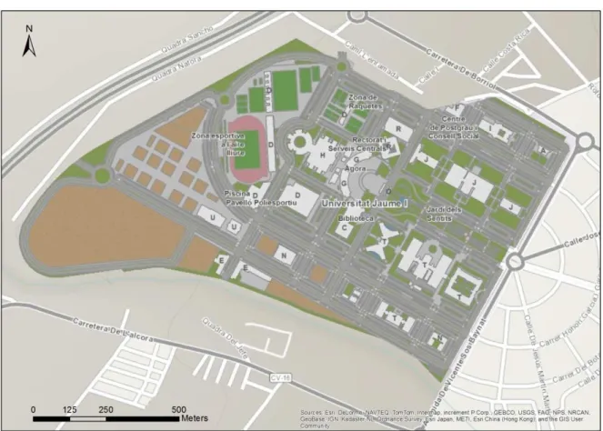
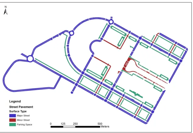
Figure 1: An overview map of the UJI Campus.
In the course of this research multiple issues came up in relation to modeling existing GIS datasets with CityEngine. Hopefully the experience of the authors as geographers and GIS users of many years will be beneficial to further development of CityEngine.
The project has been divided into two parts and this part will focus on following issues:
• Modeling of the campus basemap
The basemap will be made up of three datasets, street network (lines), landscape areas (polygons) and Streets and pavements (polygon).
• Indoor mapping
3
2. Theoretical Framework
It has been stated that spatial datasets are in some way special, that they display certain characteristics that are different from other types of data. The most obvious example of this is Toblers first law of geography: “everything is related to everything else, but near things are
more related than distant things” (Tobler, 1970). The specialty of geographical data has
prompted a whole new software industry focusing on specifically on it, the GIS industry. The industry traces its roots back to the 1960s when it the Atlas of Great Britain and Northern Ireland revealed that the only way to efficiently manage geographical data is with the help of computer databases. (Coppock et. al., 1991).
In the 1980 the software producer ESRI got the lead on designing GIS software by exploiting the relational database model for storing geographical data as vector data. This model worked well for environmental and resource management but as the technology advanced there was an increased demand for new data types that did not fit well into the current model. Urban planners for example were looking for ways of utilizing GIS within their profession (Zlatanova, et. al., 2002). At the same time new database technology was influencing database design, the shift was from relational databases to object orientated databases. Topology is one of the things that make GIS data special and is directly related to Toblers first law of geography. The new object orientated database model had a higher computational cost so topology was set up in such a way that the user has to choose if he wants to use it or not. The older systems could do this on the fly but the benefit of this design was particularly important when it comes to 3d since the typical 3d computer model is composed of objects. (Goodchild, 2003).
4
6.1.
Looking ahead
Today there is an ongoing race among designers of GIS software’s for coming up with the best functioning full 3d GIS software. To achieve this two main issues must be overcome: 1. How is 3d topology implemented?
2. What type of data structure is best suited for 3d objects?
Sisi Zlatanova points out that “The most critical difference of GIS compared to other software has always been the possibility to perform spatial analysis and visualize them. This
means practically that the models (topology, geometry, network, spatial occupancy
enumerations, free form surfaces etc.) have to be first agreed upon” (Zlatanova, 2009). This
has not happened yet although we have seen some development taking place among separate developers.
2.1.1. Data structures and types
So far there has not been a universally adopted data type for 3d GIS in the same way as the ESRI shape file vector model became the unofficial standard for 2d GIS data. There have been numerous researches on the issue and at least 14 different types of data have been proposed. They can be organized into four main categories:
• Representation 3d objects by its boundaries.
• Representation 3d objects by voxel elements.
• Representation 3d objects by a combination of the 3d basic block.
• Combined models.
5
utilize geographical coordinates (Nilsen, 2007), when used solely for the purpose of visualization this method is very effective. When on the other hand we need to design multiple objects that all have to have a single unique identifier for querying and other analysis the situation becomes more complicated and has not yet been sufficiently solved.
2.1.1. The multipatch
Today most 3d GIS models lack functionalities such as querying 3D objects, and 3D analyses such as overlay, 3D buffering and 3D shortest route (Stoter et. al., 2003). This is due to the way 3d objects are generated with the polygonal modeling technique. The standard way has been to build up 3d models from geometrical objects and link them together in a local coordinate system; as a result a single cube for example consists of 12 polygons. It then becomes obvious that to setup a query on a house that is made up of 12 or more polygons becomes complicated.
This issue becomes apparent when one thinks about topological relation of such an object, one polygon of the house might be located inside another but not the remaining. Makers of GIS software have been faced with this problem for some time now and GIS vendor ESRI has come up with a promising solution to this issue, the multipatch. The multipatch is a traditional 3d object made up of triangles, circles and arcs, the shapes are connected inside the geodatabase and as a result the 3d object appears as a single object in the attribute table. In theory this is a solid 3d object but unfortunately topology has not been developed for this model yet in the current 10.1 release of ArcGIS (ArcGIS Resouces, 2009).
Once you have a 3d solid object in the database it should be relatively easy to start building tools for analysis, this has not happened either unless to a very limited extent. 3d analysis tools have until now been centered on visualization rather than numerical data with tools such as skyline analysis and others.
2.1.
Mass 3d modeling
6
looking into solving this problem by looking at the 3d gaming and animation industry. The industry has for a long time been demanding a tool that can create a realistic 3d model of a city on a large scale efficiently.
In paper from 2001 Pascal & Yoav presented a new way of modeling whole cities in a semi automatic way with software they called CityEngine. CityEngine uses modified L-systems to grow street networks; the space in between them is subdivided into lots which are then further subdivided into shapes. Such a network can be set up in a few minutes with the automation process but if the user wants to influence it he can create the network manually. The shapes and the street network are then assigned specific set of shape grammar rules that define the shape and texture of the buildings that will be generated from the shapes (Parish & Müller, 2001). The use of shape grammars is ideal for the generation of 3d GIS models since they can take 2d shapes and generate a 3d shapes from them. CityEngine natively supports the import of the ESRI shape files and other geographical datasets such as rasters, this ensures that existing 2d data will not have to be redesigned for the 3d use.
2.2.
Shape grammar
7
8
3. CityEngine
CityEngine has established itself well within the gaming industry since its commercial release in 2008. The software has been used extensively to create highly detailed 3d model of fictional cities and urban landscapes. CityEngine has the option of importing various forms of geographical and architectural datasets such as GIS and CAD, its possibilities of modeling real landscape are quite promising. However the most efficient and widely utilized way to use the software has been to start an empty
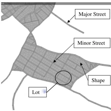
scene and let the software grow the landscape with minimal user input. After growing the streets CityEngine creates lots in between them and then divides the lots into polygon shapes (figure 1). The user can then assign a CGA (computer generated architecture) rule file to each of these polygons shapes. The CGA rule file is the actual definition of each building where it is defined with shape and split grammars.
There are three types of patterns the user
can select when generating a city this way: Organic, raster and Radial. The Organic method creates streets that have the characteristic of old medieval city and look like small clusters that grew into a bigger city. The Radial method is based on cities like Paris where the city evolved from a centre point, not uncommon where cities evolved as a fortress surrounded by a city wall. The last one the raster option create a city that looks like it was planed from the very beginning, where parallel streets cross at more or less 90° angle, New York has been used as an example of such a city. The user also chooses from these patterns a pattern for minor streets that surround the lots where the building will be created. The lots can then have recursive subdivision, skeletal subdivision, offset subdivision or no subdivision depending on the style the user wants to achieve. The user can also use height maps and obstacle maps to limit the city; the use of population data is also acceptable to influence street growth patterns (Maren et. al., 2012; Parish. et. al., 2001).
Lot
Major Street
Shape Minor Street
9
2.1. The user interface
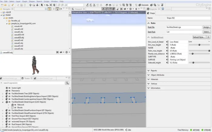
CityEngines user interface (figure 3) is a well laid out and designed for use on a large or multiple screens. The software has many advanced functionalities running under the surface while the user interface is relatively user friendly. This chapter provides a short description of the user interface and the most important components used to generate the model. Figure 3 shows a screen shot of the main user interface and how its components are laid out and will be used in the following short description.
3.1.1.
The navigator
In the top left corner of the user interface is the navigator which is CityEngines file manager. The root of the file manager is the workspace folder and when a new CityEngine project is created a folder is created in the workspace with standard CityEngines folder structure.
10
3.1.2.
The preview window
Below the navigator is the preview window where the user can preview all data formats that city engine can read. Examples would be 3d models like .obj files, most image formats including .jpeg, .tiff, .png and various other such as shapefiles and ESRI file geodatabases.
3.1.3.
The scene editor
Below the preview window is a tabbed space that holds the scene editor among other interfaces. When the user opens a scene the different layers of the scene are displayed in the scene editor tab. The user can expand each layer to display a list of all its shapes and networks, also all static models are accessible here.
3.1.4.
The rule editor
The rule editor is displayed as a different tab in the same tab space as the scene editor. It is a simple text editor for creating and modifying CGA rules but can also be used to edit all text files such as .txt or .mtl.
3.1.5.
The viewport
One of the most important part of the user interface is the viewport located at the middle of the screen. This is the window where the user can visualize and manually edit the models. In the viewport shapes can be selected for editing and CGA rule assigning. New shapes are created here and imported shapes can be transformed to static model for manual editing. The viewport has several different viewing perspectives and users can also define visual effects but the more graphics the slower the performance.
3.1.6.
The inspector tab group
11
3.1.7.
The console and scripting
In the far right tab space is also the console window and most usable part of it the python console. The python console is a useful tool to run scripts most notably if the user wants to select objects by attributes. There is no tool for selecting shapes by attributes but this can be achieved with the python console by running the following script:
ce = CE()
def selectByAttribute(attr, value):
objects = ce.getObjectsFrom(ce.scene) selection = []
for o in objects:
attrvalue = ce.getAttribute(o, attr) if attrvalue == value:
selection.append(o)
ce.setSelection(selection)
if __name__ == '__main__': pass
To simplify the process of running these scripts a helper script file can be created with the text editor and it should be saved at default script location (workspace/scripts), it can then be linked to from the python console. The above code should be saved as .py file in the script folder then the path to it is loaded into the system as follows:
sys.path.append(ce.toFSPath("scripts"))
The script is then imported:
import scriptName
12
scriptName.selectByAttribute("attributeName", "attributeValue")
13
4. Methods
This chapter is divided into three main sections; the first one is on the projection of the ViscaUJI geodatabase and how to make it compatible with CityEngine. The second one is on the creation of a base layer for the campus grounds and the third chapter is on the creation of an indoor map of the Rectorate building at the UJI campus.
4.1.
Setting up the projection
The ViscaUJI geodatabase coordinate system is the WGS 1984 Web Mercator Auxiliary Sphere with the EPSG code 3857 which is currently not supported by CityEngine. The solution is to convert the data to a coordinate system that CityEngine supports. The closest one is the WGS 1984 World Mercator coordinate system with the EPSG code 3395. The simplest way to do this is create a new file geodatabase that contains all the feature datasets we plan to use in our 3d model using in ArcCatalog. For the fastest conversion new database is created containing a feature dataset named FacilitiesStreets with the WGS 1984 World Mercator coordinate system. The following datasets are then imported from the ViscaUJI into it:
1. FacilitiesStreets/LandscapeArea.shp (Original). 2. ViscaUJI/FacilitiesStreets/Tree.shp (original).
3. ViscaUJI/FacilitiesStreets/StreetPavement.shp (needs to be modified first, see chapter 4.2).
4. ViscaUJI/FacilitiesStreets/BuildingInteriorSpace.shp (original).
14
Figure 4: The datasets used in the base layer.
4.2.
The base layer
ViscaUJI has two main polygon layers that make up the base layer for the campus grounds. They are the LandscapeArea and StreetPavement contained within the FacilitiesStreets dataset. They can be imported directly into CityEngine using the GDB importer, but before doing so some modifications must be made to it. The dataset has to be added to ArcMap and the following adjustments have to be performed on it:
The street dataset in now ready select new CityEngine Project in this case is SmartUJI and cl There are several ways of imp best is by copying the databa window open up the data fold the database and select import file GDB import must be chos and click next. The next scree selected, if selected CityEngin will distort the model.
In this project a mixed method with a street network layer. T textures to the street polygon centerline and other markings more efficiently if they are rep After analyzing the data visua on the UJI campus all categori
Figure 6: The 12 polygons that nee
15
ady for CityEngine and the next step is to start i ect and click next. The project should be assig click finish.
importing a geodatabase into CityEngine, the m base to the data folder of the project. Then g older (it might need refreshing after copying th
ort. CityEngine does not automatically detect th osen and then click next. Select all the data and reen presents several cleanup options and none gine will try to merge vertices to make them les
hod for the basemap model is used by combini . This method was chosen because it is very gons of the StreetPavement layer in order to ngs on polygon layers. City Engine can deal represented as networks using the modern street ually it becomes clear that there are indeed thr orized as one data type named street:
Figure 5: The polygons operation
need to be cut
rt it up and go to file, signed a name which
e method that works go to the navigator the data) right click t the data type so the and from chapter 4.1. ne of them should be less complex but this
ining polygon layers ry difficult to apply to maintain correct al with streets much eets template.
three types of streets
16
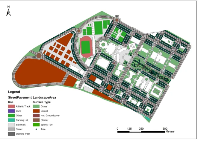
• Major roads, made up of four lanes two in each direction and in some cases lead into roundabouts.
• Minor roads, made up of two lanes one in each direction.
• Parking space roads, no lanes.
The first two types in figure 7 are exactly the once the modern streets dataset can model but the roads in the parking spaces have no chance of being modeled by it. This is due to fact that in some cases they have angles and shapes that cannot be interpreted by a line. On the other hand the roads in the parking spaces have no centerline or other markings so they can be assigned an asphalt textures later on. The decision was then made to delete all polygons representing major and minor roads from the StreetPavement layer and create a graph network in the empty spaces. In the LandscapeArea layer there so called planters in the center of the major roads and they also need to be deleted since the modern streets template generates these planters as parts of the street network graph.
17
4.2.1. Building the street network graph
Now a new network graph has to be created from the layer menu of CityEngine and it should be digitized in the middle of the empty spaces where the street polygons used to be. The width of each segment has to be set to a size that overlaps or touches the sides of the planters in the LandscapeArea layer. It is critical that the width overlaps the edges just barely and the sidewalks left and right attributes be set to 0 since they will be generated later on. Table 1 gives an overview of a typical street segment attribute for network graph, figure 9 is an example of how the resulting graph segment should look like.
Table 1: Typical attributes for the graph networks segments
Attribute Major road Minor road
shapeCreation true true
streetWidth 17.8 9.1
sidewalkWidthLeft 0 0
sidewalkWidthRight 0 0
precision 0.5 0.5
Figure 9: Example of how the street network graph must fit tightly inside the LandscapeArea layer.
18
It is desirable that the vertices of the network graph are as few as possible although multiple vertices are unavoidable everywhere the streets have curves since city engine does not deal effectively with curves in graph networks. In all locations where the pavement polygon touches the street is a walking path and at those locations vertices must frame the path as seen in figure 8.
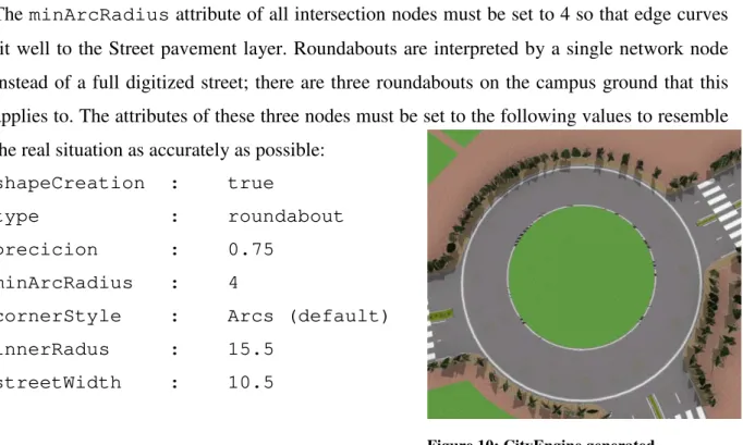
The minArcRadius attribute of all intersection nodes must be set to 4 so that edge curves fit well to the Street pavement layer. Roundabouts are interpreted by a single network node instead of a full digitized street; there are three roundabouts on the campus ground that this applies to. The attributes of these three nodes must be set to the following values to resemble the real situation as accurately as possible:
shapeCreation : true
type : roundabout
precicion : 0.75 minArcRadius : 4
cornerStyle : Arcs (default) innerRadus : 15.5
streetWidth : 10.5
The completed network graph is shown in Figure 11, on inspection notice the small dead end street that connect to the parking lot. They should have the same street width as the minor roads and just barely overlap the parking space road polygon as it will be layered on top of it.
Figure 11: The completed network
.
19
20
4.2.2. Assigning the Modern Streets template to the graph
Next the Modern Street Template was assigned to the newly created graph network. The template was downloaded at:
http://www.arcgis.com/home/item.html?id=6e45334d75f5423f9e44436cd0f53183 but it is also possible to find it through CityEngines help menu. The zip file contains all the files needed to assign textures and objects to the street network. It has the standard folder structure and was extracted to the projects root folder. The whole street network was selected and in the inspector window the ModernStreet.cga rule files was assigned to it. The start rule Street had to be manually assigned to the network since no start rule is defined for the rule file. Before generating the streets the rule attributes for the network where set to the following values:
Model Options
Level_of_detail : Low (optional)
Street Layout
Nbr_of_left_lanes : 2 Nbr_of_right_lanes : 2
Lane_width : 3
Median_width : 2
Lawns : true
Arrow_marking : true
Crosswalk
Crosswalk_width : 0
Crosswalk_style : European (not used)
Lights
Traffic_lights : true
Lamps : true
21
Trees
Tree_percentage : 100
Tree_distance : 1
Tree_max_height : 1
Traffic Density
Vehicles_per_km : 10
Bus_Percentage : 0
Sidewalk (not used)
People_percentage : 0
Props_percentage : 0
Sidewalk_height : 0
Connected Attributes(calculated by CityEngine and should not be modified)
connectionEnd : -
connectionStart : -
type : -
elevation : -
Similarily the rule attributes for the minor streets should be the following:
Model Options
Level_of_detail : Low (optional)
Street Layout
Nbr_of_left_lanes : 1 Nbr_of_right_lanes : 1
Lane_width : 3
22
Lawns : false
Arrow_marking : true
Crosswalk
Crosswalk_width : 0
Crosswalk_style : European (not used)
Lights
Traffic_lights : false
Lamps : false
Lamp_distance : 0
Trees
Tree_percentage : 0
Tree_distance : 0
Tree_max_height : 0
Traffic Density
Vehicles_per_km : 10
Bus_Percentage : 0
Sidewalk (not used)
People_percentage : 0
Props_percentage : 0
Sidewalk_height : 0
Connected Attributes (calculated by CityEngine and should not be modified)
connectionEnd : -
connectionStart : -
23
elevation : -
Two new rules had to be added to the ModernStreets.cga rule file, one to model crosswalk over major streets (the zebra rule) and one to model crosswalks over minor streets (the red brick rule). The Modern Street template has an automatic way of generating crosswalks but they are too far off from the actual crosswalks of the UJI campus. As a result all Crosswalk_width attributes where set to 0 and the ModernStreet.cga rule file was opened for editing in the rule editor and the following rules were created:
• The red brick rule
All crosswalks over minor streets are paved with red bricks instead of the standard Modern Streets template zebra crosswalk. A red brick texture image was downloaded from the internet and saved to streets folder for use with the network..
At line 167 in the modernStreet.cga rule file the texture was defined as:
24
redBrickTexture = "streets/redPavementTexture2crop.jpg"
At the end of the rule file a new rule was set up with the code:
RedPavement-->
texture("redBrickTexture") tileUV(0, ~1, ~1)
The texture command sets the texture to the one defined at line 167; the tileUV operation is defined by three integers. The first one instruct the machine to use color map, ~1 and ~1 instructs the machine to use more or less the original texture x and y sizes and tile them. This rule was then set to all minor road crosswalks that where framed in part 4.2.1.
• The zebra rule
The zebra crosswalk is automatically generated by the Modern Streets template for the major roads but does not fit to the real situation at UJI as result it was decided to manually create a rule for it.
In this rule the zebra walkway texture from the Modern Streets template was used, found in assets/streets/crosswalk.png. As before the texture was defined now in line 168 as:
modifiedZebraCrosswalk = "assets/streets/crosswalk.png"
WalkingPath -->
texture("modifiedZebraCrosswalk ") alignScopeToGeometry(zUp, 0, longest)
25
26
4.2.3. Creating a cga rule file for the LandscapeArea layer
A CGA (computer generated architecture) file is text file used to declare shape and split grammar rules for use in CityEngine. This chapter will describe in details how to CGA rule file was created for the LandscapeArea polygon layer. The LandscapeArea layer serves this purpose well since it has both simple and complex shapes that need to be modeled. The shapes are the following:
• Grass (simple texture rule)
• Gravel (simple texture rule)
• Sports Turf (simple texture)
• Ivy / Groundcover (Complex object)
• Planter (Complex object)
From the file menu a new CGA rule was created and given the name facilitiesStreet. A good practice is to divide the rule file into areas where each code type belongs to based on their functionalities. A typical CGA rule file has attributes, constants, functions textures, assets and rules. The facilitiesStreet file has attributes, textures and rules organized in the following way:
/**
* File: facilitiesStreet.cga * Created: 24 Jan 2013 21:28:56 GMT * Author: Kiddi
*/
version "2012.1"
#####################Attributes####################### Here we define our attributes
#####################Textures######################### Here we define our textures
27
In order to refer to the object attributes they had to be declared in the same manner as rule attributes. The object attributes where declared as an empty string since they already had an attribute as follows:
attr SURFTYPE = ""
By declaring the SURFTYPE attribute which classifies the polygon types it becomes usable within the rule file. Another attribute had to be declared but this time a rule attribute that set the sidewalk height above the streets:
attr Sidewalk_height = 0.2
The layer has the polygon type planter it is a big tree pot that surrounds the streets on the campus area. ViscaUJI has a tree layer but no trees are in the database for these trees so they had to be added to the planter. The trees were borrowed from the Modern Street template and added to the planter. They are Elm trees and need to have a max height and a distance rule attributes:
attr Elm_max_height = 5
attr Planter_tree_distance = rand(1,3)
The attributes where then categorized for the purpose of easy reading in the inspector by adding the following code before the attributes where declared:
@Group("Name of category")
For further visualization a code was added for mouse over messages that where displayed once the mouse sits over the attribute in the inspector with the code:
@Description("text")
28
The next part of the rule file is the definition of textures to be assigned to the LandscapeArea and it has three types:
• Grass
• Gravel
• Curb
As before the textures where downloaded from the internet and they saved to the assets project folder. The textures where defined as follows:
grass_texture = "assets/textures/grassTiles.jpg" gravel_texture = "assets/textures/gravel.png" curb_texture = "assets/streets/curb.png"
The next part of the rule is defines all assets used in it in much the same way as we as the textures where defined. The assets used where 3d models of trees that came with the Modern Street Template in the .obj format. There are several type of trees in the Modern Street Template and they were randomly generated by using the fileRandom function built into CityEngine:
Elm_Tree = fileRandom("assets/trees/alleyTree_*_v1.obj")
In most cases the assets where adjusted later on to whatever context they were used. Rules were created later in the project to further define the behavior of the trees in the planter rule. The next step was to create the actual rules that control the transformation of the shapes. The decision was made to create a so called start rule that was applied to each shape. The idea behind the start rule is to let CityEngine automatically identify the shape and assign it a
29 secondary rule which defines its behavior. The secondary rules vary considerably depending on the object they are intended to model so it is important that the start rule identifies the object correctly. The start checks the SURFTYPE attribute and assigns it the correct secondary rule for the shape; this is achieved with a simple switch loop. The start rule is declared with the
@StartRule function followed by its name and the symbol -->
@StartRule StartRule -->
The switch loop:
Case SURFUSE == "Grass" : grassRule
Case SURFUSE == "Gravel" : gravelRule
Case SURFUSE == "Sports Turf" : grassRule
Case SURFUSE == "Planter" : planter
Case SURFUSE == "Ivy / Groundcover" : planter
else : NIL
There are three secondary rules presented here, two of them are simple texture rules but the planer rule is a little more complicated. The following section explains in detail each operation of these three rules.
In the course of this description if an operation has been covered previously it will not be explained again but assumed that the reader is already familiar with it.
30
• The texture rules; grassRule and gravelRule
Grass -->
At first the up axis of the scope is set to z and the scope aligned to the shapes longest edge:
alignScopeToGeometry(zUp, 0,longest)
Set the scope of the projection:
setupProjection(0,scope.xz,scope.sx,scope.sz)
Project the texture space onto the object (UV)
projectUV(0)
Define which texture to use:
texture(grass_texture)
Then texture space was tiled approximately (~1 stands for more or less one to one ratio) in its original size (higher values stretch the image):
tileUV(0, ~1, ~1)
This code is a simple way of defining textures for a shape from a polygon layer and can be used exactly the same way with the gravel texture except texture used is different.
• The planter rule
The planter is an area surrounded by curbs and has gravel at the bottom and trees growing on the inside (see figure 19). These planters are defined as polygons in ViscaUJI and they need to be elevated into 3d space by extruding:
31
Planter -->
extrude(Sidewalk_height)
This operation creates a 3d object from the selected shape and the height of the object is defined by the Sidewalk_height attribute set earlier. The object is defined to have faces and each face is worked on separately. The extruded 3d objects can either be split by vertices, faces or edges, here the object is split into two faces: sides and bottom using the comp(f) operation:
comp(f) { side : BorderNormal | bottom : reverseNormals BottomNormal PlanterTreesNormal }
Since only the sides and the bottom are defined with the comp(f) function only those facades are displayed, the one remaining façade the top is discarded and not displayed. Inside the curly braces is where the facades are defined, after the colon sign any operation can be defined but usually only references to another rule is placed here as is the case with the side rule. The bottom face starts with the operation reverseNormals which is necessary since the textures and objects attached to it apply on the outside of the object by default. The BottomNormal and PlanterTreesNormal are rules that define the bottom texture and trees which will be created later.
setupProjection(0,scope.xz,scope.sx,scope.sz) projectUV(0)
• The Border rule
Figure 19 shows that the sides of the planter are large concrete stones and a rule was created to model them. This rule is the one applied to the sides in the comp(f) split of the planter rule:
BorderNormal-->
s('2, Sidewalk_height*4, Sidewalk_height*4)
32
The s operator sets the scope (size) of the object in the x, y and z order which is the default order used in all geometry operations. The x size is set to a value of absolute 2 which splits the border into two unit sizes (scale factor is unknown) and the absolute value instructs the program to cover all the area. The borders extrude from the sidewalk and have the same width as height so the y and z values were set as multiplication of the Sidewalk_height. In this case the multiplication factor is 4 to ensure the borders where always four times higher than the sidewalk.
t(-0.2, 0, -Sidewalk_height*4)
The t operator shifts the border a little bit to align the edges, x axis -0.2, y axis does not change and the z axis is shifted to align up with x axis in proportion with the Sidewalk_height.
i("builtin:cube")
The i operation imports the object that all these operations apply to, in this case the built in cube object.
Curbs2
At last the Curbs2 texture rule was assigned to the new shape, the Curbs2 rule is a simple texture rule with the scope set to the absolute value of 1 for x and z axis.
• The BottomNormal rule
The BottomNormal rule is referenced by the planter rule and is a normal texture but it was manipulated a little too raise it above the pavement texture that in some cases lies under it.
t(0,0,-Sidewalk_height*1.5)
This operation ensures that the bottom texture is always elevated 6 mm over the sidewalk texture.
• The PlanterTreesNormal
Inside the planter are trees that were imported objects and they needed to be distributed:
PlanterTreesNormal
alignScopeToGeometry(yUp, any, longest) t(0,0,0.9)
33
| 0.1: Elmtree | ~ Planter_tree_distance *0.5 : NIL }
This rule splits up the texture space (the bottom) along the longest edge and places empty space based on the Planter_tree_distance attribute at the shortest edge. Then it inserts an Elm tree at the next point by referring to the Elm tree rule and places an empty space besides it. Multiplying the operation by itself generates a repeat of the pattern that fills up the whole planter with trees.
• The Elmtree rule
The final piece of the puzzle is the rule that imports the elm tree object:
Elmtree -->
s(0,Elm_max_height,0)
Sets the height of the tree to the Elm_max_height attribute the width attribute was kept at 0 in order for the tree to scale itself proportionally to the height.
r(0,rand(0,360),0)
Rotates the tree randomly around the y axis, the x and z where kept at 0 for the trees to stand upright.
i(ELM)
Imports the elm tree from previously defined assets.
There is another type of plan point feature with the exact lo was created. That planter is of planterTreesNormal rule but w
4.2.4. Creating a c
The other part of the base lay shares some textures with the rule file but to add the rules to assigned to the layer in the sa order to only have to manipula inspector window it affects StreetPavement layer are the fo
• Street (Simple texture)
• Curb (Extruded texture
• Walking path (extruded
• Sidewalk (extruded tex
• Parking Lot (Color onl Figures 23 to 25 show exampl red and grey color but it was d scope of this project to split th
Figure 22: The resulting planter a
Figure 23: the texture used for the Sidewalk and curb.
34
nter on the UJI campus that also contains tr location of those trees in which case a planter of the type Ivy / groundcover and it uses an id t without trees.
cga rule file for the StreetPavement
layer is made up of the StreetPavement polygo he LandscapeArea layer so it was decided not t
to the already existing facilitiesStreet rule file same manner as to the LandscapeArea layer. T
ulate one sidewalk_height attribute, when it is cts the whole base layer as a result. Th e following: re) ure) ded texture) texture) nly)
ples of the textures used, note that the paveme s decided only to use one red tile texture. It wo the pavement into red and gray areas.
r after applying the planter rule to it.
Figure 24: the texture
used for the walking path. Figure for the
trees. There exist a ter rule without trees identical rule as the
nt layer
gon layer. The layer to create a separate . The rule was then r. This was critical in is manipulated in the The objects of the
ment of UJI has both would be beyond the
35
Majority of the polygons in this layer are textures and need no explanation although the sidewalk needed a little modification. The texture definition for those polygons was the following:
grass_texture = "textures/grassTiles.jpg" asphalt_texture = "assets/streets/asphalt.png" gray_tiles_texture =
"textures/brick_pavement_0022_03_preview.jpg"
Also most of the streets polygons were generally assigned the asphalt rule from modernStreets.cga rule file (the rule was copied to the facilitiesStreet rule file) there was an exception on two polygons that represent a double zebra walkway. The big exception was the planter type in the layer that had to be assigned a planter rule similar as the one in chapter 4.2.3. The street polygons and the planter rule will be explained in the next chapter but an important difference of the StreetPavement layer is the attribute used to categorize the dataset is SURFUSE but not SURFTYPE as in the LandscapeArea layer. The SURFUSE object attribute must be declared in the facilities rule the same way as was done for the SURFTYPE object attribute. Then all the polygon types of the StreetPavement layer were added to the switch loop in the start rule. All the rules for the objects here are simple texture rules and follow the same principals as the texture rules already mentioned. However the sidewalk needed to be extruded just a little bit and needs simple border for decoration with the following rule:
Pavement -->
alignScopeToGeometry(yUp, 0, longest)
setupProjection(0,scope.xz,scope.sx,scope.sz) projectUV(0)
extrude(Sidewalk_height)
comp(f) { side : Curbs2 | top : PavementText }
First the texture definition was added to texture section of the rule file:
red_brick_texture = "streets/redPavementTexture2crop.jpg"
36
4.2.5. The double walking path and parking lot planter
There are two cases on the UJI campus where a walking path crosses a parking lot street polygon and the walking path has a double zebra markings (see figure 27). The double zebra had to be identified in the StreetPavement layer and its SURFUSE attribute was changed to doubleWalkingPath to separate it from the standard streets (See figure 26).
The double zebra texture was created from the zebra texture supplied with the modern street template in the Gimp photo editor and the texture definition was added to the rule file:
double_walking_path = "streets/doubleCrosswalk.png"
A new rule was created at the end of the facilitiesStreet.cga rule file for the double zebra.
The double walking path starts with the same code as the walking path rule of the street network, but since it is a polygon further functions were added:
setupProjection(0, scope.xy, '1, '1)
Instructs CityEngine to use colormap, the object scope is in the xy plane (horixontal) and the ratio between axes is absolute one to one.
projectUV(0)
Creates the final texture coordinates of the UV-set by applying the corresponding projection matrix.
rotateUV(0,90)
Rotates the UV-set 90° for perfect fit.
Figure 26: The double zebra polygon with the texture assigned to it.
37
There are 12 polygons in the middle of all round parking spaces that represent planters that are in reality exactly like the planters in the previous example. However ViscaUJI has a layer called trees which contains the exact location of some trees including those in the parking lot planter. To generate an accurate model these tree points where used where they were available and a new rule created for the parking lot planter without the automatic generation of trees. The exact same rule was used but instead of using the split operation:
comp(f) { side : BorderNormal | bottom : reverseNormals BottomNormal PlanterTreesNormal }
the split operation:
comp(f) { side : BorderNormal | bottom : reverseNormals BottomNormal }
was used.
The 12 polygons where selected and their object attribute SURFTYPE changed from Planter to PlanterParking and the new planter rule assigned to them.
Figure 28: A street wiew from the UJI campus after generating the rules.
38
4.3.
Indoor mapping
There is no general procedure for generating indoor 3d. maps in CityEngine and this chapter describes the process of creating a 3d indoor map for the rectorate building at the UJI campus. The goal was to create a map of the building that can be viewed from the outside to the inside using data from ViscaUJI that was created from CAD files.
4.3.1. Data preparation
In the ViscaUJI database there are two feature layers named buildingInteriorSpace and buildingFloorplanPublish. The feature layers are detailed architectural floor plans for each floor of five buildings on the campus area, each floor is categorized in the field floor. The values range from S (sub floor), 0 – 6 and C (Cubierta in Spanish or roof in English). The datasets were added to ArcGIS for modification before they could be worked on in CityEngine. The rectorate building was selected in both datasets and exported from the dataset as a two shapefiles for each dataset. When the Rectorate was exported successfully from building interiorSpaces it needed no further editing and was ready to be imported into CityEngine, the buildingFloorplanPublish needed more work though.
Figure 30: Indoor spaces sub floor.
Figure 32: Indoor spaces second floor
Figure 34: The sub floor shell.
Figure 37: The second floor shell.
39
Figure 38: The third floor shell.
Figure 31: Indoor spaces
ground floor Figure 2floor
Figure 33: Indoor spaces third floor
Figure 3 Figure 35: The ground floor
shell.
Figure 36
29: Indoor spaces first
40
4.4.1. The outer shell
Once the data had been imported to CityEngine a new rule file was setup in the same manner as was done in the previous examples. As before a switch loop was used for a start rule which identified each floor, extruded them and stacked them on top of each other with the t function.
The attribute used for identifying the floors is the FLOOR object attribute and had to be declared as an empty string. A rule attribute was created to control the height of the floors with name floorHeight and its default value set to 4. The basic structure of the switch loop is the following:
case FLOOR == "S" : extrude(-floorHeight) t(0, -4, 0)
case FLOOR == "0" : extrude(floorHeight) t(0, 0, 0)
case FLOOR == "1" : extrude(floorHeight) t(0, floorHeight, 0)
case FLOOR == "2" : extrude(floorHeight) t(0, floorHeight*2, 0)
case FLOOR == "3" : extrude(floorHeight) t(0, floorHeight*3, 0)
case FLOOR == "roof" : extrude(floorHeight/2) t(0, floorHeight*4, 0)
else : NIL
41
the circle where there is only supposed to be one. The same happens with the columns but they are ignored here and we will focus on the big circle and the same method can be used for them. The comp(f) split function can be used for the sub, ground, first and second floors as follows:
comp(f) { world.north : wallLong | world.south : wallLong | world.east : wallLong | world.west : wallLong }
This code split the sides of each floor depending on which direction they face and assigned them the wallLong texture rule.
What had to be done for the third floor on the other hand was a different approach, the floor was split by faces but instead of indentifying them by direction each face is assigned a number by CityEngine and assigned to it. Each line between vertices is in fact a face and in this case over 60 faces are identified just for the third floor and they all had to be assigned textures:
comp(f) {
2 : tile | 3 : wallLong | 4 : wallLong | 5 : tile | 6 : tile | 7 : tile | 8 : tile … }
42
4.4.2. The interior
The same principles outer shell was followed for the generation of indoor spaces. The BuildingInteriorSpace layer is divided into floors in the same manner as buildingFloorplanPublish layer so a switch loop was created as a start rule. As usually few things had to be inserted to the rule file before the start rule. The interior map was decorated with people models taken from the modern streets template, the following assets where therefore added to the assets part of the rule file:
peopleAsset =
fileRandom("assets/people_by_lowpolygon3d_com/*.obj")
This line randomly chooses a human model from the various ones supplied with the Modern Streets template.
dirHuman = 50%: 90 else: -90
43
This line was put for later reference and it randomly rotates the models. The walls inside the rectorate are around 15 cm thick and a infinitely thin polygon line is inefficient to
intemperate them. To make the interior walls thicker a the following rule was added:
Wall -->
s('1, floorHeight, 0.15)
Sets the scope to the full extent of the polygon layer, the height was set to the floorHeight and wall thickness is set to 0.15 meters.
i("builtin:cube")
Imports the built in cube and applies them to the polygon layer
color(1,1,1)
The last one is optional but in this case the walls were assigned color with the value 1,1,1 which is white (default)
To add the people models to the indoor model the following rule was created:
Human -->
alignScopeToAxes(y) t(3,0,'rand(0.1,0.6))
The t (translate) function is not new but here it uses the rand function to generate objects randomly inside the object scope in this case on the y-axis.
s(0,rand(1.7,1.9),0) r(0,dirHuman,0)
The r (rotate) function is already known but here it uses the dirHuman attribute to rotate the models randomly around the y axis.
i(peopleAsset)
The last part is sets up a switch loop for the different floors that controls the extrusion and splits the shapes into faces:
Lot -->
caseFLOOR == "IS" : extrude(-floorHeight) comp(f) {side : Wall}
44
caseFLOOR == "I0" : extrude(floorHeight) comp(f) {side : Wall | bottom : Human} t(0, 0, 0)
caseFLOOR == "I1" : t(0, floorHeight, 0) extrude(floorHeight)
comp(f) {side : Wall | bottom : Human}
caseFLOOR == "I2" : t(0, 2* floorHeight, 0) extrude(floorHeight)
comp(f) {side : Wall | bottom : Human}
caseFLOOR == "I3" : t(0, 3* floorHeight, 0) extrude(floorHeight)
comp(f) {side : Wall | bottom : Human}
45
46
5. Discussions
CityEngine is a powerful software package for creating realistic 3d models. The program is well suited for generating 3d content from conventional 2d GIS data types such as ESRI shapefiles and geodatabases. The following two chapters address separately the strong and weak points of the software suite from a geographers and the GIS users perspective:
5.1.1. Strong points
One of CityEngines main strong features is the ability to generate large 3d models of cities on the fly. If the user is working with building footprints of building that contain the building heights in an attribute table a low level model of large city can be generated in a few minutes with decent a computer. Such a model could for example instantly be used for skyline analysis. The user also has full control over which parts of the city he wants to add details either by using the manual the editing tools or rule based. The procedural modeling with cga shape grammar rules needs a minimal knowledge of programming and is good starting point for geographers who are more and more being forced to learn scripting languages in their use of GIS. The option of defining building parameters through attributes and modify them in the navigator resulting in instant visibility is a clever way of making programming visual.
The user interface is rich and has many good editors one of them is the façade wizard that allow you to edit a façade visually and generate from your edits a rule to apply to facades. There is also a feature of CityEngine that is called crop image tool, although not used in the generation of the streets it is a convenient way to edit texture and facade images without having to switch to dedicated image processing software. The built in shapes of the program are vital for the generation of indoor walls, curbs, railing and other smaller details of models and hopefully they will increase in future versions.
5.1.2. Weak points
47
cases more recent geodatabases contain objects that made up of arcs which in turn are generated from only endpoints (ArcGIS Resources, 2013a). CityEngine however does not have this function and when such a curve is imported that curve is generated as a straight line between the two endpoints. The way around this problem is to add points to the curve until with such a small space between them that they resemble a curve and can be very time consuming. Another issue on related to shapes is in regards to the manual editing tool which is missing a feature to create round shapes. As with the arcs if you want to add for example a column footprint for extrusion that has to done with straight lines in tight formation until they resemble a circle. The manual editing too is also missing other vital components such as a measuring tool to verify the dimensions of the designs. Snapping is automatic when editing manually and should be an option as it is in ArcGIS especially since it is not yet possible to create arcs and points are needed to be inserted in rapid succession. Full support to all projected coordinate system is still missing. Recently web projections have been redefined to WGS 1984 Web Mercator Auxiliary Sphere with the WKID is defined as 3857. The ViscaUJI geodatabase uses this projection also but it has not been included into CityEngine which is a big flaw since datasets are increasingly being made for the web. Although it is possible to select objects by attributes using python scripting it would be a nice feature to able to set up selection query similar to once ArcGIS has.
48
49
6. Conclusion
When this project started the author had no knowledge on CityEngine other that it could be used to generate 3d city models. The objective was to create a 3d model of the University Jaume I Campus and look into the possibilities of joining it up with the Smart UJI project. The software performed well in the generation of the model itself. The program has the typical learning curve where as the author was slow in adopting the many possibilities of it but as time progressed they became somewhat of experts on its many functions. Given the six month assigned to this project and delays for one month due to licensing issues it can be said that the most of the objectives were address although some of them were not satisfactorily concluded. There exists now a model prototype of the university campus that can still be further developed down to its last detail. It has been shown that the program can be used to create nice looking indoor maps but still there are unresolved issues with indoor assets such as spiral staircases.
50
rectorate demonstrates this very well where a single polygon represented a single room of the building was extruded and the top removed, the resulting multipatches could be queried as single objects.
51
Bibliography
ArcGIS Resources (2013a). ArcGIS Help 10.1 - Creating a curve through endpoints (Endpoint Arc) Viewed January 10, 2013 at
http://resources.arcgis.com/en/help/main/10.1/index.html#/through_endpoints_Endpoint_Arc/01
m70000006n000000/
ArcGIS Resouces (2013b). ArcGIS for Local Government 10.1 . Viewed January 10, 2013 at
http://resources.arcgis.com/en/help/localgovernment/10.1/index.html#/Welcome_to_ArcGIS_for
_Local_Government_online_help/028s00000023000000/
ArcGIS Resouces (2009). Forum Thread: Beta 10: Topology in ArcGlobe. Viewed January 16, 2013 at http://forums.arcgis.com/threads/1370-Beta-10-Topology-in-ArcGlobe
ArcGIS Resources, (2012). Example Modern Streets 2012 Viewed November 19, 2012 at http://www.arcgis.com/home/item.html?id=50e9b9b6c3ea4617b5b4a7bfd4e7f38c
Cheng, R. (2012). Google unveils full 3D Google Earth feature. Viewed January 12, 2013 at
http://news.cnet.com/8301-1023_3-57448299-93/google-unveils-full-3d-google-earth-feature/
Coppock J.T. & Rhind D.W. (1991). The History of GIS. in Maguire D.J., Goodchild M.F.,
Rhind D.W. (editors), Geographical Information Systems : Principles and Applications (pages 21-43). Longman Scientific: Essex
Elwannas, R. (2011). 3D GIS: It's a Brave new World. Speech made at The Sixth National GIS
Symposium in Saudi Arabia. Viewed at
http://www.gdmc.nl/3dcadastres/literature/3Dcad_2011_04.pdf
Esri (2008). The Multipatch Geometry Type [ESRI whitepaper]. California: ESRI Press
Goodchild, M., F. (2003). Finding the mainstream. Keynote speech at the Map India Conference, New Delhi.
Handrahan, H. (2011). Games Industry International Esri acquires CityEngine developer Procedural.
Viewed Desember 26, 2013 at
http://www.gamesindustry.biz/articles/2011-07-12-esri-acquires-cityengine-developer-procedural
Hohmann, B., Havemann, S., Krispel, U., Fellner, D. (2010). A GML shape grammar for semantically
52
Maren, G. V., Shephard, N., Schubiger, S. (2012). Developing with Esri CityEngine Viewed September 29 at
http://proceedings.esri.com/library/userconf/devsummit12/papers/developing_with_e
sri_cityengine.pdf)
Muller, P., Wonka. P., Haegler, S., Ulmer, A., Gool, L. V., Leuven, K. U. (2006). Procedural modeling
of buildings. ACM Transactions on Graphics, 25(3), 614 - 623
Nielsen, A. (2007). A Qualification of 3d Geovisualization. PhD thesis, Aalborg University, Aalborg.
Parish, Y. I., & Müller, P. (2001). Procedural modeling of cities. Proceedings of the 28th annual conference on Computer graphics and interactive techniques (pp. 301-308). New York: ACM.
Stiny, G., Gips, J. (1972). Shape Grammars and the Generative Specification of Painting and
Sculpture. Information Processing 71, 1460-1465.
Stoter, J. & Zlatanova, S. (2003). 3D GIS where are we standing? Joint Workshop on Spatial, Temporal and Multi-Dimensional Data Modelling and Analysis, 2-3 October, Quebec city,
Canada.
Tuan, A. N. G. (2013).Overview of Three-Dimensional GIS Data Models. International Journal of Future Computer and Communication, 2(3), 270–274
Tobler, W., R. (1970). A Computer Movie Simulating Urban Growth in the Detroit Region. Economic Geography, 46, 234-240
Watson, B., Müller, P., Wonka, P., Sexton, C., Veryovka, O., Fuller, F. (2008).
Procedural Urban Modeling in Practice. Computer Graphics and Applications, 28(3) 18-26.
Wonka, P., Wimmer, M., Sillion, F., Ribarsky, W. (2003) Instant Architecture. Transactions on Graphics 22(3), 669-677
Yin, X., Wonka, P., Razdan, A. (2009). Generating 3D Building Models from Architectural
Drawings: a survey. Computer Graphics and Applications, 9(1). 20-30
53
Zlatanova, S., Rahman, A. A., Pilouk, M., (2002). Trends in 3D GIS development. Journal of Geospatial Engineering, 4(2), 1-10
54
Annex A
/**
* File: facilitiesStreet.cga * Created: 24 Jan 2013 21:28:56 GMT * Author: Kiddi
*/
version "2012.1"
#####################Attributes#######################
attr SURFTYPE = "" attr SURFUSE = "" attr NAME = ""
attr Sidewalk_height = 0.04
attr Elm_max_height = 5
@Range("Low","High")
attr Elm_Level_of_Detail = "Low"
attr Palm_max_height = 10
const highLOD = Elm_Level_of_Detail == "High"
attr Planter_tree_distance = rand(1,3)
########################Textues##########################
curb_tex = "assets/streets/curb.png" double_walking_path = "streets/doubleCrosswalk.png" gravel_texture = "assets/textures/gravel.png" grass_texture = "textures/grassTiles.jpg" gray_tiles_texture =
"textures/brick_pavement_0022_03_preview.jpg"
asphalt_texture = "assets/streets/asphalt.png"
######################Assets############################# ELM =
case highLOD :
fileRandom("assets/trees/tree_eu03_11_*.obj") else :
fileRandom("assets/trees/alleyTree_*_v1.obj")
PALM = "assets/trees/myPalm4.obj"
##########################Rules########################