Bayesian binary regression model: an application to in-hospital death after AMI prediction

BAYESIAN BINARY REGRESSION MODEL: AN APPLICATION TO IN-HOSPITAL DEATH AFTER AMI PREDICTION

Aparecida D. P. Souza *

DMEC / Faculdade de Ciências e Tecnologia Universidade Estadual Paulista (UNESP) Presidente Prudente – SP

adps@prudente.unesp.br

Helio S. Migon

DME / Instituto de Matemática e

Programa de Engenharia de Produção / COPPE Universidade Federal do Rio de Janeiro (UFRJ) Rio de Janeiro – RJ

migon@pep.ufrj.br

* Corresponding author / autor para quem as correspondências devem ser encaminhadas

Recebido em 07/2003; aceito em 04/2004 Received July 2003; accepted April 2004

Abstract

A Bayesian binary regression model is developed to predict death of patients after acute myocardial infarction (AMI). Markov Chain Monte Carlo (MCMC) methods are used to make inference and to evaluate Bayesian binary regression models. A model building strategy based on Bayes factor is proposed and aspects of model validation are extensively discussed in the paper, including the posterior distribution for the c-index and the analysis of residuals. Risk assessment, based on variables easily available within minutes of the patients’ arrival at the hospital, is very important to decide the course of the treatment. The identified model reveals itself strongly reliable and accurate, with a rate of correct classification of 88% and a concordance index of 83%.

Keywords: mortality probability prediction; model selection in binary regression; model diagnostic and residual analysis.

Resumo

Um modelo bayesiano de regressão binária é desenvolvido para predizer óbito hospitalar em pacientes acometidos por infarto agudo do miocárdio. Métodos de Monte Carlo via Cadeias de Markov (MCMC) são usados para fazer inferência e validação. Uma estratégia para construção de modelos, baseada no uso do fator de Bayes, é proposta e aspectos de validação são extensivamente discutidos neste artigo, incluindo a distribuição a posteriori para o índice de concordância e análise de resíduos. A determinação de fatores de risco, baseados em variáveis disponíveis na chegada do paciente ao hospital, é muito importante para a tomada de decisão sobre o curso do tratamento. O modelo identificado se revela fortemente confiável e acurado, com uma taxa de classificação correta de 88% e um índice de concordância de 83%.

1. Introduction

The main objectives of the paper are to show how easy it is to handle Bayesian analysis of the binary regression model using Gibbs sampler and to illustrate some aspects of model building, diagnostic checking and residuals analysis. The new developments of stochastic simulation almost eliminate the difficulties associated to the Bayesian analysis of non-linear models, including binary regression models.

A Bayesian model building strategy parallels to Hosmer & Lemeshow (1989) is proposed. Bayes factor is used for the selection of variables or to discriminate among competitive models. Numerical aspects of the evaluation of the predictive distribution are also considered.

The main diagnosis measures presented in this paper are the c-index and the models rate of correct classification. Their full posterior distributions are easily assessed via MCMC. The c-index represents the proportion of times in which the probability of in-hospital death is smaller in the survivors group than in the deaths group. The predictive rate of correct classification is the proportion of patients correctly allocated to the death and survival groups. Jointly those measures allow to evaluate the predictive ability of the model. The Bayesian residual analysis is based on an approach proposed by Albert & Chib (1995), which consists in obtaining the posterior distribution of the parametric residual, represented by the difference between the individual’s answer for the variable of interest and his estimated probability.

Several studies have assessed the factors related to mortality prognosis after acute myocardial infarction. The main problem the physician faces is to predict, in an emergency context, the death risk for a patient after arriving at the hospital having suffered from an acute myocardial infarction. The values of some variables easily available upon the patient’s admission are recorded together with clinical characteristics in order to precisely evaluate the in-hospital death probability. The assessment of such risk is very important for the decisions in the course of treatment, the alternative therapies and the use of clinical resources. Mortality predictors can allow physicians to be more efficient in assessing risk-benefit when faced with therapeutic decisions.

In a prospective study involving 546 consecutive outpatients after acute myocardial infarction, variables related with mortality were observed and provide the data to be analyzed throughout this paper illustrating some methodological issues in binary regression.

This paper is organized as follows. Bayesian binary regression model is summarized in the next section, including some aspects of Gibbs sampling. Model building strategy is introduced in Section 3. The data set and the main findings are carefully described in Section 4. The diagnostic checking and a residual analysis are presented in Section 5 and the paper finalizes with some concluding remarks in Section 6.

2. The Bayesian Binary Regression Model

The binary regression model (Collet, 1994), is used to explain the probability of a binary response variable as function of some covariates. The model is specified by:

| ( ),

i i i

where y_i=1 if the response of interest is observed for the ith individual and zero otherwise,

i

π is the probability that the ith individual presents the response under investigation, β is the K vector of unknown parameters, xt_i =(x_i1,...,x_iK) the K vector of known covariates associated to the ith individual and F any transformation assuming values in (0, 1). For instance, the function F can be any arbitrary cumulative distribution function. The most useful specifications of F includes the logistic, the normal and the extreme value, that is:

t t i i t t i i t i

exp( ) /[1 exp( ], _{( )}

( ) ( ), ( )

exp[ exp( )].

logistic

F probit

(complementary log - log)

 +



= Φ

 ₋  x x x x x β β) β β 1− β

The link function defines the linear predictor as:

1

1 1

( ) ...

i F i xi KxiK

−

= = + +

η π β β . (1)

For each of the three models stated above the linear predictor is respectively: log(π_i/(1−π_i)), Φ(π_i) and log( log(1− −π_i)). The model choice depends on the relation between the response variable and the covariates. Some practical recommendations about the model choice and numerical examples can be found in Collet (1994) and Dobson (2002).

The likelihood function for data y= (y ,..., y_{1 n})t is:

(1 )

t t

i i

1

( | ) [ ( )] [1i ( )] i . n

y y

i

p y β F F −

=

=

∏

To progress with the Bayesian analysis it is necessary to provide a joint prior distribution over the parameter space. This is very hard to do as far as the relationship between the data and the parameters is very complex. The easiest way to circumvent this difficult is to propose a informative prior, but with small precision, avoiding any complaint about the specification of subjective beliefs (O’Hagan et al., 1991). In this paper, informative independent normal priors, with extremely small precisions, were set to the parameters. Therefore,

(1 )

t t

i i

1

( ) ( ) [ ( )] [1i ( )] i . n

y y

i

pβ y p β F F −

=

| ∝

∏

Clearly (3) is a complex function of the parameters and numerical methods are needed in order to obtain the marginal posterior distribution for each of the model parameters. Approximations can be obtained via Laplace methods (Tierney, Kass & Kadane, 1989) or numerical integration (Naylor & Smith, 1982). Simulation based methods have proliferated in the last ten years or so yielding two popular approaches known as importance sampling (Zellner & Rossi, 1984) and Gibbs sampling (Dellaportas & Smith, 1993, and Albert & Chib, 1993). Resampling techniques, applied to logistic regression for randomized response data, were alternatively proposed by Tachibana & Migon (1995).

denominated adaptive rejection method, (Gilks & Wild, 1992) to obtain r, 1,...,

k k= K

β and

1,...,

r= R, where R is the Monte Carlo sample size. The posterior distribution of any statistic of interest, function of the parameters, for instance the probability of death, the concordance probability (c-index) or the rate of correct classification, is easily obtained from the sample drawn via the MCMC methodology.

The Gibbs sampler was implemented easily through the software BUGS – Bayesian Inference Using Gibbs Sampler (Spiegelhalter et al., 1995). The number of iterations demanded for the indication of convergence of the sampler was defined through the diagnostics of Raftery & Lewis (1992). The diagnostics of Geweke (1992) and an analysis of the behavior of the chains along the iterations were also used for this end. Considering these criteria, the results presented in the next sections are based on a long run, with the 10 initial iterations discarded to allow the burn-in and the next 6000 stored for the sample.

3. Model Building

Strategy for model building usually involves seeking the most parsimonious model that still is able to explain the data. Overfitting a model could produce numerically unstable estimates characterized by large estimated standard errors. In binary regression, model building involves the selection among non-nested models (the link function), besides the choice of the best subset of variables. Furthermore, in a full Bayesian approach, we should elicit prior information on the regression coefficients. The easiest way to do that is, firstly, to elicit prior information about the in-hospital mortality and later on to derive a prior distribution on the regression coefficients, as proposed by Bedrick, Christensen & Johnson (1997). This approach assures that the prior effect is in some sense invariant to the link function selection.

Although the above described strategy is completely general and can be applied to binary regression with any chosen link function, we will illustrate in this paper only a variable selection strategy in the case of the logit link function. The main reason why logistic regression has proven to be such a powerful analytic tool for medical research is the interpretability of the regression coefficients as log odds.

Selection procedures like stepwise, best subset, etc., have been criticized in the literature because they can yield a medical implausible model and can select irrelevant variables. In this paper, the Hosmer & Lemeshow (1989) strategy is applied after slight modifications giving a Bayesian flavor to the previous variable selection proposal. The main steps involved are:

i) begin with univariate analysis to select the main risk factors;

ii) fit a multivariate logistic regression to the covariates previously selected;

iii) fit new multivariate models excluding in each step, one at a time, the covariates with high posterior density interval (HDI) including zero;

iv) test, one at a time, the variables excluded in step (i) as well as other relevant clinical covariates using the same criterion as above;

v) evaluate the need to add non-linear terms and interactions; vi) compare competitive multivariate models using the Bayes factor.

Bayes factor for comparing models Ml e MS are numbers Bl S, such that

,

( _l| ) / ( _S| ) _{l S} ( _l) / ( _S)

p M y p M y =B p M P M ,

where p M( _l) and p M( _S) indicate the priori odds for each model. The Bayes factor is a multiplier that changes the priori odds for the models into the posterior odds. Applying the theorem of Bayes it can be shown that

, ( | ) / ( | )

l S l S

B =p y M p y M ,

where p( |y M) is the marginal probability of obtaining y from model M. Computing ( | )

p y M for a model M involves integrating the corresponding likelihood function with respect to the induced prior on β for that model.

4. The Data Set and the Main Findings

A sample of 546 outpatients with 73 deaths were consecutively observed in the admission of Procardiaco Hospital at Rio de Janeiro, Brazil, from January 91 up to December 95. The data set consists of demographic and medical variables observed at the admission of patients after AMI. The primary end point of the trial was in-hospital death from any cause. Additional details about the protocol guiding this experiment can be found in Bassan et al. (1996).

The models developed in this paper are based on a set of eleven variables previously selected from the main study. These are the factors usually recommended in the medical literature to predict the in-hospital mortality (Greenland et al., 1991). Most of these variables can be evaluated as soon as the patient arrives at the hospital. The variable AGE is continuously measured by years. The others, are mainly dichotomous variables: SEX coded as 1 for male and 0 for female, HAS, IAMP, DIAB and SMOKE set as 1 meaning the presence of history of arterial hypertension, previous myocardial infarction, diabetes and the habit of smoking, respectively, and 0 meaning absence. From the admission electromagnetic exam the AMI was classified as non-inferior, inferior or lateral and described by the following zero-one variables: PAREA – non-inferior, PAREI – inferior and PAREL – lateral. An alternative way is to classify the AMI by the absence of the Q-waves (PARES). Additionally, the congestive failure scaling known as class Killip on admission (KILLIP), an ordinal measure of the intensity of the infarction, is measured in a scale varying from 1 to 4.

The main findings obtained following the proposed model building strategy were:

i) the covariates AGE, SEX, IAMP, PAREI, SMOKE e KILLIP were firstly selected to explain the in-hospital death, based on an univariate analysis;

ii) the multivariate logistic regression model including the above covariates was fitted to the data (M1). The 95% HDI calculated for the coefficient of the covariate PAREI contained

the null value, indicating that it is not statistically significant to predict in-hospital mortality, in the presence of the other mentioned variables;

iv) the next step involved the fit of multivariate models including, one at a time, the covariate excluded from the previous step, HAS, DIAB, PAREA, PAREL and PARES. At this stage, only the covariate HAS is statistically relevant in the presence of the others (M₃);

v) an investigation for non-linearity in the relationship involving AGE and KILLIP confirmed the linearity found in the fit of the model.

Models including second, third and fourth order interactions were also analyzed. One of the selected models (M₄) includes the main effects and interactions terms like AGE x HAS, SEX x HAS and HAS x IAMP. The model (M5) exploring third order interactions, involves

the terms HAS x IAMP, HAS x SMOKE, IAMP x SMOKE and HAS x IAMP x SMOKE.

The Bayes factor used to choose the best model is presented in Table 1. As suggested by Kass & Raftery (1995) there is a substantial (subs) evidence against model MS (in favor of

l

M ), when log (₁₀ B_{l S,} )∈(0.5,1.0). When log (₁₀ B_{l S,} )∈(1.0, 2.0) the evidence is called strong (str) and if it is bigger than 2, decisive (dec). It is easy to see that model M₁ is not preferred to M2, confirming that PAREI is not an effective risk factor. On the other hand,

the model M₃ is better than M₂ showing how significant the variable HAS is. Finally, the model M4 is preferred when compared with M3 and M5.

Although the coefficients of the covariates AGE and SMOKE are not statistically different from zero (the 95% HDI are (-0.002, 0.051) and (-1.410, 0.107), respectively for AGE and SMOKE) these two covariates are kept in our basic model (M3) because they are clinically

relevant. Furthermore, using the sampled values of the β ’s we evaluate the probability of

smoke

β being greater than or equal to 0 as 0.052, and the probability of βage being less than or equal to 1 as 0.035. These figures clearly show that the HDI must be used with caution.

The model selection computations were performed approximating the marginal probability for the harmonic mean of the likelihood with sampled parameters values of the posterior distribution. In agreement with Kass & Raftery (1995), this approach is very easy to calculate, and experience to date suggests that although it is indeed unstable, it often results that are accurate enough for interpretation on the logarithmic scale. Thus, given a sample

, 1,..., r

r= R

β from posterior, for model M,

1 1

1

1

( | ) ( | )

R

r

r

p M p

R

y y β

− −

=

 

=  



∑

Table 1 – Approximate Bayes Factor for Model i Against Model j.

Model

(l,S) log10Bl S,

Evidence Against M_S

2, 1 0.328 null

3, 2 0.564 subs

4, 3 0.960 subs

In Table 2, the posterior mean for the parameters of the selected model (M₄) obtained via Gibbs sampler and also the maximum likelihood estimate are presented including its standard deviation. There are no strong differences between the MCMC and the MLE estimates certainly because the sample size is large enough and the prior is informative, but with smaller precision. In Figure 1 the entire posterior distribution can be appreciated including the corresponding HDI. The Bayesian analysis presents the advantage of allowing the obtaining of distributions of functions of the parameters, such as the c-index and the rate correct classification presented in the section 5.

The inclusion of the interaction terms made the model more powerful as can be seen in Table 1. It is important to emphasize that although for some covariates the null value pertains to the 95% HDI, they are considered clinically relevant and, therefore, maintained in the model.

Table 2 – Model M₄ Estimated Coefficients and Standard Deviation.

Variable Gibbs Sampler Coef (se)

MLE Coef (se)

CONST -5.80 (1.46) -5.74 (1.41)

AGE 0.05 (0.02) 0.05 (0.02)

SEX -1.45 (0.44) -1.41 (0.43)

HAS 2.22 (2.08) 2.45 (1.95)

IAMP 0.19 (0.49) 0.20 (0.48)

SMOKE -0.67 (0.40) -0.61 (0.38)

KILLIP 1.47 (0.20) 1.42 (0.20)

AGE x HAS -0.05 (0.03) -0.06 (0.03)

SEX x HAS 0.63 (0.66) 0.61 (0.64)

IAMP x HAS 1.09 (0.70) 1.05 (0.68)

The odds ratio, adjusted to other factors in the model, is defined by

1 1 1 1 1 1

1 1 1 1 1 1

exp( ... ... )

( ) exp( )

exp( ... ... )

k k k k k K K

k k

k k k k K K

x x x x

x

x x x x

− − + +

− − + +

+ + + + + +

Ψ = =

+ + + + +

β β β β β _β

β β β β ,

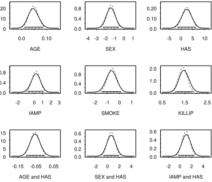
where xk =0 or 1 represents an unit variation in xk, for the continuous case, or the presence or absence of the factor, in the discrete case. It is mainly used in the medical literature as a useful measure to interpret the parameters. The posterior distributions of the odds ratios for the main factors in this application are presented in Figure 2 (full line) together with the asymptotic distributions of the maximum likelihood estimators (broken line). Although the posterior distributions for the odds ratios for AGE, SEX (female) and IAMP are slightly skewed, its mode and the high posterior density intervals are similar to the asymptotic one.

The simultaneous effect of each of those factors and HAS can also be examined in Figure 2. The following comments are based on the mean value of the odds ratios and on the 95% probability intervals presented inside brackets:

ii) the effect of AGE decreases to Ψ= 0.97 (0.64, 1.44) in the presence of hypertension; iii) the mean odds ratio for female SEX is Ψ= 4.69 (1.75, 9.93) indicating that in-hospital

mortality is 4.69 times more frequent among women. This figure reduces to 2.56 (0.87, 6.01) in the group of hypertension women;

iv) IAMP, in the presence of hypertension has mean odds ratio, Ψ= 4.068 (1.41, 9.50), while for non-hypertension patients this figure decays to 1.36 (0.45, 3.00);

v) considering a 60-years-old patient, the odds ratio for HAS is Ψ= 0.48 (0.12, 1.35), providing evidence that the presence of hypertension is somewhat like a protection factor. The same happened with SMOKE, Ψ= 0.555 (0.230, 1.10);

vi) the risk of death increases by a factor of 4.45 (Ψ= 4.45 (2.97, 6.56)) for each unitary variation on Killip.

Those results permit to conclude that AGE, IAMP in the presence of hypertension, the female sex and Killip measured at admission are risk factors while the male sex and the habit of smoking represent protection for the in-hospital death.

AGE 0.0 0.10 0

10 20

SEX -4 -3 -2 -1 0 1 0.0

0.4 0.8

HAS -5 0 5 10 0.0

0.10 0.20

IAMP

-2 0 1 2 3

0.0 0.4 0.8

SMOKE

-2 -1 0 1

0.0 0.4 0.8

KILLIP

0.5 1.5 2.5

0.0 1.0 2.0

AGE and HAS -0.15 -0.05 0.05 0

5 10 15

SEX and HAS -2 0 2 4 0.0

0.2 0.4 0.6

IAMP and HAS -2 0 2 4 0.0

0.2 0.4 0.6

AGE (10 years) 1 2 3 0.0

0.5 1.0 1.5

Female SEX 0 5 10 15 20 0.0

0.10 0.20 0.30

IAMP 0 2 4 6 8 0.0

0.4 0.8

AGE (10 years) and HAS 0.5 1.0 1.5 2.0 0.0

1.0 2.0

Female SEX and HAS 0 5 10 15 0.0

0.2 0.4

IAMP and HAS 0 10 20 30 0.0

0.10 0.20 0.30

HAS and AGE (60 years old) 0 1 2 3 0.0

1.0 2.0

SMOKE 0.0 1.0 2.0 0.0

1.0 2.0

KILLIP 2 4 6 8 10 0.0

0.2 0.4

Figure 2 – Posterior Densities of the model M₄ Odds Ratios. Gibbs Sampler (full line); Asymptotic distribution (broken line).

5. Model Diagnostic and Residual Analysis

Typically a fitted model must be evaluated by its predictive capacity. A well-known measure for this purpose is the concordance index, which will be defined in this Section. Its posterior distribution will be assessed from the MCMC sample. Additionally, the posterior distribution of the rate of correct classification based on a particular cut-off point is also presented. To illustrate the strength of the selected model, a comparative boxplot of the π’s for the two groups: survival and non-survival is exhibited.

These statistics are functions of the estimated probability of hospital death for each patient, which is, in its turn, obtained as function of the simulated β’s via Gibbs Sampler.

5.1 The c-index

Let πi₁ and πj2, i=1,...,n j1, =1,...,n2 be the death probabilities for the

th

i non-survival

patient (group 1) and jth survival patient (group 2), respectively. The ‘c-index’ (Pryor, 1993) is defined as C=P[π_death>π_survival| ]y . In order to estimate this quantity let

1 2

1 2

1 if 0 if

i j

ij

i j

C =  > < 

π π

π π ,

where πi1 and πj2 are the sampled death probabilities for each of the two groups. The

‘c-index’ posterior distribution can be evaluated using Gibbs sampling as:

1 2

1 1

1

, 1,..., n n

r r

ij i j

C C r R

n = =

=

∑∑

where n=n₁+n₂ and R is the MCMC sample size.

In this application the posterior mean of the ‘c-index’ was Cl= 0.83, with a 95% high posterior density interval (0.82, 0.84). These results can be better appreciated in Figure 3(a), where the exact posterior density obtained via MCMC can be compared with the asymptotic normal approximation for the distribution of a jackknife estimator. It is worth pointing out that the confidence interval based on jackknife is much wider than that one based on Gibbs sampler. The Bayesian approach considers all of the involved uncertainties and allows to obtain the true posterior distribution.

The c-index is a measure of the area under the curve ROC – Receiver Operating Characteristic (Hanley & MacNeil, 1982), that is, it represents the relationship between the conditional probabilities denominated sensibility and specificity. The sensibility represents the probability of predicting death given that the patient died and specificity the probability of predicting survival given that the patient survived

5.2 The rate of correct decisions

The distributions of the fitted π’s for the two groups: survival and non-survival are presented in the boxplots of Figure 4. For the first group, the first quartile, the median and the third quartile are respectively (0.024, 0.044, 0.086), meanwhile for the second group the corresponding quantities are (0.093, 0.291, 0.704), providing evidence for the model capacity to separate the patients with different outcomes. Moreover, the outliers that appear in the survivors’ group represent incorrect classifications, which could be justified for complications occurred during the internment period and not detected in the patient’s admission.

With the same purpose, the distributions of the rate of correct decisions, Figure 3(b), shows that 88% of the patients were correctly classified assuming a cut-off point π0= 0.40. This

Evidently, incorrect classifications in the two directions have different costs. To predict high death probability erroneously can take to applications of unnecessary clinical resources, offering risks to the patient and elevating the cost of the treatment. On the other hand, to predict small death probability erroneously can take for the not use of necessary resources and unfortunately to the patient’s death.

c-index

0.78 0.82 0.86 0.90 0

10 20 30 40 50 60

(a)

rate of correct classification 0.84 0.88 0.92 0

10 20 30 40 50 60

(b)

Figure 3 – (a) Posterior Densities of the model M4 c-index. Gibbs Sampler (full line); Jackknife Method (broken line); (b) Posterior Density of the Model M₄ Rate of Correct Classification via

Gibbs Sampler.

0.0 0.2 0.4 0.6 0.8 1.0

survival

0.0 0.2 0.4 0.6 0.8 1.0

non-survival

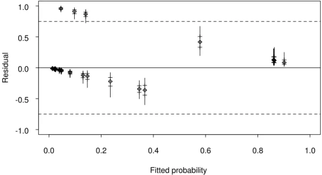
5.3 The residual analysis

Figures 5 and 6 present the marginal posterior densities of the residuals ri =yi−πi, for each patient in randomly selected sample of size 30. The range of values of the posterior distribution of ri is determined by the observed yi, the interval (0, 1) when yi =1 and the interval (-1, 0) when y_i =0. In Figure 6, the boxplots of the residuals are plotted against the fitted probabilities. The general aspect of the graphic in Figure 6 is similar to the one obtained when the frequentist residuals for binary data are plotted. The posterior medians fall inside the two parallel lines corresponding respectively to the responses y_i =1, the upper one, and yi =0, the lower one.

The shape of the distribution of the residuals depends on its location. Outlier observations correspond to marginal densities located far away from zero, concentrated at the extremes of the possible value range of the residuals and showing strong asymmetry.

Albert & Chib (1995) suggested to evaluate the posterior probabilities of ri=k, for some arbitrary constant k. The boxplots for the patients number 46, 48 e 59, with extreme probabilities 0.9543, 0.9915 and 1.000, respectively, cross the parallels corresponding to the 0.75 (Figure 6). For the other patients this probability are smaller than 0.005. Although these probabilities are efficient in the identification of candidates to be outliers, the choice of the k value is subjective.

The files of these patients with high probability were carefully investigated and some mistakes were sorted out. Patient number 59 was wrongly registered as an in-hospital death and the class Killip for patient number 48 was assessed as being smaller than it really was. After considering these modifications, keeping the records of patient 46 unaltered, the final model (M₄) was refitted providing almost the same results.

Residual

Pos

terior dens

ity

-1.0 -0.5 0.0 0.5 1.0

0 10 20 30 40 50

48

59 46 57

47 44 52

Fitted probability

Resi

dual

0.0 0.2 0.4 0.6 0.8 1.0 -1.0

-0.5 0.0 0.5 1.0

Figure 6 – Boxplots of the Residuals versus Fitted Probabilities for each of 30 patients randomly selected.

6. Concluding Remarks

A simple approach to a Bayesian analysis of the Bernoulli regression was presented in this paper. A slight modification on the variable selection strategy proposed by Hosmer and Lemeshow was outlined based on the Bayes factor and high posterior density interval concepts. Another practical contribution for model diagnostic was the evaluation of the posterior distribution for the c-index based on the simulated sample. The residual analysis follows the suggestion made by Albert & Chib (1995). Some alternative proposals were under consideration at the time this paper was being written.

The model developed is capable to predict in-hospital mortality of patients with AMI accurately. Mortality prediction can allow physicians to be more efficient in assessing risk-benefit ratios in these patients. The selected risk variables, all easily available in the admission, including female gender, age, absence of history of hypertension, history of previous infarction and Killip class. The cumulative effect of those variables indicates increasing mortality rate. The preferred model includes some second order interaction factors involving HAS, SMOKE and AGE, making it strongly non-linear. The model reliability was assessed through a careful residual analysis. The ability of the model to discriminate between patients with and without the outcome of interest was assessed by a c-index of 0.83 and a rate of correct classification as large as 0.88.

Acknowledgments

References

(1) Albert, J.H. & Chib, S. (1993). Bayesian Analysis of Binary and Polychotomous Response Data. Journal of the American Statistical Association, Theory and Methods, 88(422), 669-679.

(2) Albert, J.H. & Chib, S. (1995). Bayesian Residual Analysis for Binary Response Regression Models. Biometrika, 82(4), 747-759.

(3) Bassan, R.; Postch, A.; Pimenta, L.; Tachibana, V.M.; Souza, A.D.P.; Migon, H.S. & Dohmann, H. (1996). Hospital mortality in Acute Myocardial Infarctions: Is it possible to Predict Using Admission Data?. Arq. Bras. Cardiol., 67(3), 149-158.

(4) Bedrick, E.J.; Christensen, R. & Johnson, W. (1997). A New Perspective on Priors for Generalized Linear Models. Journal of the American Statistical Association, 91(436), 1450-1459.

(5) Collet, D. (1994). Modelling Binary Data. Chapman & Hall, London.

(6) Dellaportas, P. & Smith, A.M.F. (1993). Bayesian Inference for Generalized Linear Models and Proportional Hazards via Gibbs Sampling. Applied Statistics, 42, 443-459.

(7) Dobson, A.J. (2002). An Introduction to Generalized Linear Models. Chapman & Hall, London.

(8) Geweke, J. (1992). Evaluating the acurracy of sampling-based approaches to calculating posterior moments (with discussion). In: Bayesian Statistics 4 [edited by J.M. Bernardo, J.O. Berger, A.P. Dawid and A.F.M. Smith), Oxford University Press, Oxford, 169-193.

(9) Gilks, W.R.; Richardson, S. & Spiegelhalter, D.J. (1996) (eds.). Markov Chain Monte Carlo in Practice. Chapman & Hall, London.

(10) Gilks, W.R. & Wild, P. (1992). Adaptive Rejective Sampling for Gibbs Sampling. Applied Statistics, 41, 337-348.

(11) Greenland P.; Reicher-Reiss, H.; Goldbourt, U. & Behar, S. (1991). In-hospital and 1-year mortality in 1524 women after myocardial infarction. Circulation, 83, 484-491.

(12) Hosmer Jr., D.W. & Lemeshow, S. (1989). Applied Logistic Regression. John Wiley & Sons, New York.

(13) Kass, R.E. & Raftery, A.E. (1995). Bayes Factors. Journal of the American Statistical Association, 90(430), 773-795.

(14) Naylor, J.C. & Smith, A.M.F. (1982). Application of a Method for the Efficient Computation of Posterior Distribution. Applied Statistics, 31, 214-225.

(15) O’Hagan, A.; Woodward, E.G. & Moodaley, L.C. (1991). Practical Bayesian Analysis of Simple Logistic Regression: Predicting Corneal Transplants. Statistics in Medicine, 9, 1091-1101.

(17) Raftery, A.E. & Lewis, S. (1992). How Many Iterations in the Gibbs Sampler? In: Bayesian Statistics 4 [edited by J.M. Bernardo, J.O. Berger, A.P. Dawid and A.F.M. Smith], Oxford University Press, 763-773.

(18) Spiegelhalter, D.J.; Thomas, A.; Best, N. & Gilks, W. (1995). BUGS (Bayesian Inference Using Gibbs Sampling) Version 0.50. MRC Biostatistics Unit, Cambridge, UK.

(19) Tachibana, V.M. & Migon, H.S. (1995). Approximated Methods in Bayesian Randomized Response Models. Tech. Report, Les/UFRJ.

(20) Tierney, L.; Kass, R.E. & Kadane, J.B. (1989). Fully Exponential Laplace Approximations to Expectations and Variances of Non-positive Functions. Journal of the American Statistical Association, 84(407), 710-716.