Rosineide Fernando da Paz

Alternative regression models to Beta distribution

under Bayesian approach

PROGRAMA INTERINSTITUCIONAL DE PS-GRADUAO EM ESTATSTICA UFSCar-USP

Rosineide Fernando da Paz

ALTERNATIVE REGRESSION MODELS TO BETA DISTRIBUTION UNDER

BAYESINA APPROACH

Thesis submitted to the Departamento de Estatística - Des/UFSCar and to the o Instituto de Ciências Matemticas e de Computação - ICMC-USP, in partial fulfillment for PhD degree in Statistics - joint Graduate Program in Statistics UFSCar-USP.

Advisor: Prof. Dr. Jorge Luís Bazán Guzmán

PROGRAMA INTERINSTITUCIONAL DE PS-GRADUAO EM ESTATSTICA UFSCar-USP

Rosineide Fernando da Paz

MODELOS DE REGRESSÃO ALTERNATIVOS À DISTRIBUICÃO BETA SOB

ABORDAGEM BAYESIANA

Tese apresentada ao Departamento de Estatística - Des/UFSCar e ao Instituto de Ciências Matemticas e de Computação - ICMC-USP, como parte dos requisitos para obtenção do título de Doutor em Estatística -Programa Interinstitucional de Ps-Graduação em Estatística UFSCar-USP.

Orientador: Prof. Dr. Jorge Luís Bazán Guzmán

ACKNOWLEDGEMENTS

Os agradecimentos principais são direcionados à Deus, quando algumas vezes, sentindo-me desacreditada e perdida nos sentindo-meus objetivos, ideais ou minha pessoa, sentindo-me deu forças e sentindo-me fez acreditar em mim mesma.

Um agradecimento especial vai para o meu marido Amilton José Monteiro, que sempre esteve lá, por mim.

Agradeço aos professores participantes da banca examinadora que dividiram comigo este momento tão importante e esperado e por terem sido mediadores do meu conhecimento e terem despertado em mim a busca contínua de desenvolvimento e por informações: Artur J. Lemonte, Caio L. N. Azevedo, Heleno Bolfarine, Luís A. Milan e Jorge Luis Bazán. E em especial ao orientador dessa tese (Jorge Luis Bazán) que acompanhou todo o desenvolvimento desse trabalho.

Agradeço também a Coordenação de Aperfeiçoamento de Pessoal de Nível Superior (CAPES), pelo suporte financeiro.

ABSTRACT

PAZ, R. F. Alternative regression models to Beta distribution under Bayesian approach. 2017. 120 p. Tese (Doutorado em Estatística – Interinstitucional de Pós-Graduação em Esta-tística) – Instituto de Ciências Matemáticas e de Computação, Universidade de São Paulo, São Carlos – SP, 2017.

The Beta distribution is a bounded domain distribution which has dominated the modeling the distribution of random variable that assume value between 0 and 1. Bounded domain distributions arising in various situations such as rates, proportions and index. Motivated by an analysis of electoral votes percentages (where a distribution with support on the positive real numbers was used, although a distribution with limited support could be more suitable) we focus on alternative distributions to Beta distribution with emphasis in regression models. In this work, initially we present the Simplex mixture model as a flexible model to modeling the distribution of bounded random variable then we extend the model to the context of regression models with the inclusion of covariates. The parameters estimation is discussed for both models considering Bayesian inference. We apply these models to simulated data sets in order to investigate the performance of the estimators. The results obtained were satisfactory for all the cases investigated. Finally, we introduce a parameterization of the L-Logistic distribution to be used in the context of regression models and we extend it to a mixture of mixed models.

Keywords: L-Logistic distribution, Bounded response, Mixture model, Simplex

RESUMO

PAZ, R. F. Modelos de regressão alternativos à distribuição Beta sob abordagem

bayesi-ana. 2017. 120p. Tese (Doutorado em Estatística – Interinstitucional de Pós-Graduação em

Estatística) – Instituto de Ciências Matemáticas e de Computação, Universidade de São Paulo, São Carlos – SP, 2017.

A distribuição beta é uma distribuição com suporte limitado que tem dominado a modelagem de variáveis aleatórias que assumem valores entre 0 e 1. Distribuições com suporte limitado surgem em várias situações como em taxas, proporções e índices. Motivados por uma análise de porcentagens de votos eleitorais, em que foi assumida uma distribuição com suporte nos números reais positivos quando uma distribuição com suporte limitado seira mais apropriada, focamos em modelos alternativos a distribuição beta com enfase em modelos de regressão. Neste trabalho, apresentamos, inicialmente, um modelo de mistura de distribuições Simplex como um modelo flexível para modelar a distribuição de variáveis aleatórias que assumem valores em um intervalo limitado, em seguida estendemos o modelo para o contexto de modelos de regressão com a inclusão de covariáveis. A estimação dos parâmetros foi discutida para ambos os modelos, considerando o método bayesiano. Aplicamos os dois modelos a dados simulados para investigarmos a performance dos estimadores usados. Os resultados obtidos foram satisfatórios para todos os casos investigados. Finalmente, introduzimos a distribuição L-Logistica no contexto de modelos de regressão e posteriormente estendemos este modelo para o contexto de misturas de modelos de regressão mista.

Palavras-chave: Distribuição L-Logistica, Resposta limitada, Modelo de mistura, Distribuição

LIST OF FIGURES

Figure 1 – Histograms of the data of voting percentage obtained by PT in presidential elections, in the cities of Sergipe State, from year 1994 and 1998, when the PT lost the presidential election, to 2002,2006 and 2010, when the PT candidate was Presidential winner, and its estimated densities based on the posterior predictive distribution for 1, 2 and 3 components.. . . 38

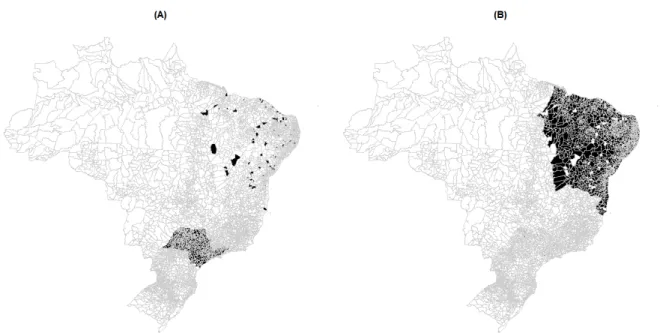
Figure 2 – Histograms and posterior density function. . . 49 Figure 3 – Real histogram and Estimated density function for the MHDI data set. . . . 52 Figure 4 – Classification of HDI of cities in the states São Paulo and Northeastern region

of Brazil where the cities classified in the second component are in black in (A) and cities classified in the first component are in black in (B). . . 53 Figure 5 – Scatter plot with marginal histograms of the data. . . 60 Figure 6 – Scatter plot of the classified data. . . 61 Figure 7 – L-Logistic probability density function for scale parameterm=0.1,0.5 and

0.7 and some values of parameterb. . . 68 Figure 8 – L-Logistic probability density function for shape parameterb=0.1,1 and 4

and some values of scale parameterm. . . 68 Figure 9 – The mode, skewness (γM and γ0.125) and kurtosis (kQ) of the L-Logistic

distribution for some values of the parameters. . . 72 Figure 10 – Descriptive measures of the L-Logistic distributions for some values of the

parameters . . . 73 Figure 11 – Estimated densities for Beta and L-Logistic models for de scenarios with

n=100,φ =10 andr=5%. . . 81

Figure 12 – Posterior predictive error bars with 95% confidence intervals of the generated values yrep_(i) versus ordered observed data y_(i) for the PPOBC data, using L-Logistic and Beta models. . . 83 Figure 13 – Estimated density of PPOBC data. . . 83 Figure 14 – Scatterplot and histograms of the real data. . . 85 Figure 15 – Standard residual versus adjusted values for the L-Logistic and Beta models. 86 Figure 16 – L-Logistic probability density function for scale parameterm=0.2,0.5 and

0.8 and some values of parameterb. . . 91 Figure 17 – L-Logistic probability density function for shape parameterb=0.5,1 and 2

of the parameters of component 2 are in black and the values of parameters of component 3 are in red. . . 99 Figure 19 – Chais values for the parameters of MLLMR model considering the data of

LIST OF ALGORITHMS

Algoritmo 1 – Algorithm for simulating samples from the posterior distribution of the parameters of the mixture of Weibull . . . 34 Algoritmo 2 – Algorithm for simulate samples from the jointly posterior distribution of

the parameters of the mixture of L-logistic regression models . . . 58 Algoritmo 3 – Algorithm for simulate samples from the posterior distribution of the

parameters of the mixture of mixed L-Logistic regression models . . . 98 Algoritmo 4 – Algorithm for simulate samples from the posterior joint probability

LIST OF TABLES

Table 1 – Twice the natural logarithm of the Bayes factor of the data of voting percentage under one model resulting of mixture of Weibull distribution relative to another. . . 37 Table 2 – Posterior mean and HPD interval of parameters of the best Weibull mixture model chosen by

Bayes factor evaluation. Data of voting percentage obtained by PT in presidential elections in the Sergipe State from year 1994 to 2010 was considered for fitting of the models. . . 40

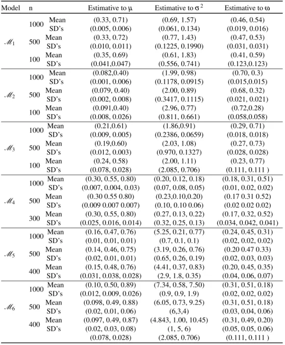
Table 3 – Parameters used to simulate the data sets and the posterior relative frequency for the number of components obtained from each simulated data set of sizen. 49 Table 4 – Posterior mean of the parameters and empirical standard deviation (SD) for

simulated data sets considering six models withk=2 andk=3 described in

Table 3. . . 50 Table 5 – Relative frequency ofkto the MHDI data set considering alternative SM models. . . 51

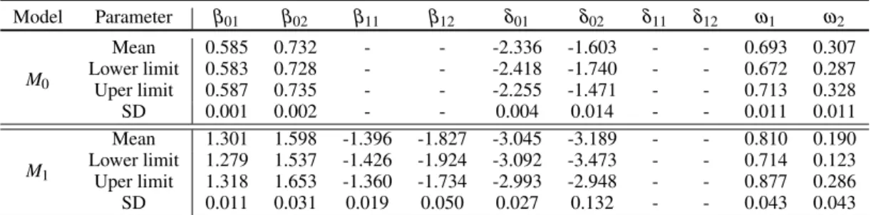
Table 6 – Posterior estimates of the parameters and the empirical standard deviation for the MHDI data set. . . 51 Table 7 – Model comparison criteria to the models proposed to MHDI data. . . 61 Table 8 – Number of observations classified across the models and components. . . 61 Table 9 – Posterior mean, credibility intervals and standard empirical deviation of the

estimated parameters for sub-modelM0andM1. . . 62

Table 10 – EY[Y],EY[Y2], andVarY(X)of the L-Logistic distribution for some values of

bandm. . . 73 Table 11 – Posterior mean with 95% HPD interval, prior distributions for parameter b

and true values of the parameters of L-Logistic distribution used to simulate the data sets. . . 78 Table 12 – Bias and root mean square error (√MSE) of the Bayesian estimator of the

parametersmandb. . . 80 Table 13 – Comparison of Bias, MSE and percentage of selection of the model L-Logistic

versus Beta considering WAIC, EAIC, EBIC and DIC for different scenarios of contaminated Beta data (two values ofφ 3% of outliers and three sample sizes) by considering 100 dataset replications in each scenario. . . 81 Table 14 – Estimates and 95% HPD intervals for the parameters of the L-Logistic and

Table 18 – Posterior mean and 95% HPD intervals for the parameters of MLLMR model applied to simulated data.. . . 99 Table 19 – Posterior mean and 95% HPD intervals for the parameters of MLLMR model

CONTENTS

1 INTRODUÇÃO . . . 23

2 A MOTIVATION: STUDY OF THE VOTES OF A BRAZILIAN

POLITICAL PARTY . . . 27

2.1 Introduction . . . 28

2.2 The votes of a political party. . . 29

2.3 The general mixture model . . . 30

2.4 The Weibull mixture model . . . 32

2.5 Choosing the number of components in the mixture model . . . . 34

2.6 Results . . . 37

2.7 Discussion and further development . . . 39

3 MIXTURE OF SIMPLEX DISTRIBUTIONS WITH UNKNOWN

NUMBER OF COMPONENTS . . . 41

3.1 Introduction . . . 42

3.2 Simplex Mixture Distribution . . . 43

3.3 Inference . . . 44

3.4 Analysis of simulated data sets . . . 48

3.5 Analysis of a municipal HDI data set in Brazil . . . 51

3.6 Final comments . . . 52

4 MODELING MHDI WITH A FINITE MIXTURE OF SIMPLEX

RE-GRESSION MODELS . . . 55

4.1 Introduction . . . 56

4.2 Model specification . . . 56

4.3 Bayesian inference . . . 57

4.4 Data analysis . . . 58

4.5 Conclusion . . . 62

5 L-LOGISTIC REGRESSION MODELS: PRIOR SENSITIVITY ANA-LYSIS, ROBUSTNESS TO OUTLIERS AND APPLICATIONS . . 65

5.1 Introduction . . . 66

5.2 The L-Logistic Distribution . . . 67

5.6 Applications to a real data set . . . 81

5.7 Final remarks . . . 87

6 FINITE MIXTURE OF MIXED L-LOGISTIC REGRESSION: A BAY-ESIAN APPROACH . . . 89

6.1 Introduction . . . 89

6.2 L-Logistic distribution . . . 90

6.3 L-Logistic median regression model . . . 91

6.4 L-Logistic mixed median regression (LLMR) model . . . 92

6.5 Mixture of L-Logistic mixed-effect models . . . 96

6.6 Remarks . . . 100

7 CONTRIBUTIONS AND FUTURE DEVELOPMENTS . . . 103

7.1 Contributions . . . 103

7.2 Future development . . . 104

BIBLIOGRAPHY . . . 105

APPENDIX A PROCEDURE FOR SIMULATE SAMPLE FROM A

MIXTURE OF SIMPLEX DISTRIBUTIONS WITH UNKNOWN NUMBER OF COMPONENT . . . 111

APPENDIX B PROOFS OF PROPERTIES OF THE L-LOGISTIC

23

CHAPTER

1

INTRODUÇÃO

Random variables with support on a bounded subset of the real line are common in practical problems and are frequently analyzed by researchers, for instance, Impartial Anony-mous Culture (STENSHOLT,1999) and the Human Development Index (HDI) (MCDONALD; RANSOM,2008;CIFUENTESet al.,2008). Examples of bounded variables which are often analyzed are rates and proportions bounded in (0,1) interval. In these case, we usually transform the variables by the logit transformation in order to deal with an unbounded variables However, some problems arise with this approach. One problem is that rates and proportions display more variation around the mean and this variation decrease in the neighborhood of the lower and upper limits of the standard unit interval. In addition an antisymmetric distributions can be more appropriate for modeling this kind of data. For modeling this kind of data, different models have been proposed in the past. For example, among others,Buckley(2003),Ferrari and Cribari-Neto (2004),Lemonte and Bazán(2016),Gómez-Déniz, Sordo and Calderín-Ojeda(2014),Bayes, Bazán and Castro(2017) andJones(2009). However, there are still continuous distributions with bounded support that need further study.

In the mixture model context, there are some studies which consider mixtures of Beta distributions (BOUGUILA; ZIOU; MONGA,2006;BOUGUILA; ELGUEBALY,2012), but other probability distributions with support in the (0,1) interval, the Simplex distribution for an example, have not yet been completely analyzed or studied. The Simplex distribution was proposed by Barndorff-Nielsen and Jorgensen(1991) and has recently been considered as a complementary and alternative regression model to the beta regression model (LÓPEZ,2013; SONG; TAN,2000). A simple advantage of the Simplex distribution is that both, mean and dispersion parameter, are shown explicitly in its probability density function. The distribution can have one or two modes, and cannot emulates a flat distribution as the uniform distribution on the interval (0, 1).

(called here L-Logistic), originally proposed by Tadikamalla and Johnson (1982). This dis-tribution was studied by, among others, Tadikamalla and Johnson (1990) and Johnson and Tadikamalla(1991), who proposed the method of moments and the percentile points method to fit this distribution. However, regression models were not studied by considering this distribution.

In this thesis, we consider the Simplex distribution and the L-Logistic distribution as alternatives to the Beta distribution in some different situations as: mixture model, regression model, among others to model data bounded in (0,1) interval. The work was motivated by the data of percentages of votes obtained by a political party in elections in different cities of an region of the Brazil seen inPaz, Bazán and Elher(2015), and described here in the Chapter2. These data sets have some characteristics of Benford’s Law (see for exempleBerdufi(2014) and Cuff, Lewis and Miller(2014b)) and recentlyCuff, Lewis and Miller(2014a) have established the relation between the Weibull distribution and Benford’s Law. Thus, the percentages of votes to each city are assumed here to follow a Weibull distribution. In this work, mixture models are also used in the analysis of the percentages of votes in order to give more flexibility for the model. These data sets are an example of data which need a more flexible distribution to be suitable modeled

The Chapters 3, 4, 5 e 6 of this thesis are based on manuscripts written to present models alternatives to Beta distribution. In the third chapter a mixture of Simplex distributions for modeling proportional data is presented. The Simplex distribution is a distribution recently studied as alternative to Beta distribution (LÓPEZ,2013;SONG; TAN,2000). However, since the data present multimodality we propose a mixture of Simplex distributions for the modeling process. A full Bayesian approach is considered in the inference process in mixture of Simplex distributions and the method adopted is theReversible-jumpMarkov Chain Monte Carlo. The usefulness of the proposed approach is confirmed by use of the simulated mixture data from several different scenarios and through an application of the methodology to analyze municipal Human Development Index data of the cities of the Northeast region and São Paulo state in Brazil. The work presented in this chapter is a manuscript published in the Journal of Applied Statistics (PAZ; BAZÁN; MILAN,2015).

The fourth chapter is dedicated to the analysis of the Municipal Human Development Index as a function of proportion of poor people per municipality. We propose a regression model where the response follow a mixture of Simplex distribution. Estimation is performed also by a Bayesian approach making use of Gibbs samplingalgorithm. For the choice of the number of component in the mixture, we make a comparison of the models with different components. This chapter present a work published as a expanded abstract for 60a_{Reunião Anual da Região}

Brasileira da Sociedade Internacional de Biometria (RBras), 2015, conference.

25

the median is an explicit parameter and we can easily write it as a function of covariates in a regression structure. If the data are highly skewed, where the median is a natural robust measure of the center, the conditional median modeling can be more useful than conditional mean modeling adopted in Beta regression models. For the model without covariate, simulation studies, considering prior sensitivity analysis and comparison with Beta distribution, give evidence that the L-logistic distribution is more robust then Beta distribution to modeling data with outliers. Applications to real and simulated data are also performed. The work presented in this chapter is under review for publication.

27

CHAPTER

2

A MOTIVATION: STUDY OF THE VOTES OF

A BRAZILIAN POLITICAL PARTY

Abstract

Statistical modeling in Political Analysis has ben used to describe electoral behavior of political party. In this paper we propose a Weibull mixture model to describe the votes obtained by a political party in Brazilian presidential elections. We considered the votes obtained by the Partido dos Trabalhadores in five presidential elections from 1994 to 2010. A Bayesian approach was considered and a random walk Metropolis algorithm withinGibbs samplingwas implemented. Next, Bayes factor was considered to the choice of the number of components in the mixture. In addition the probability of obtain 50 percent of the votes in the first round was estimated. The results show that only few components are needed to describe the votes obtained in this election. Finally, we found that the probability of obtaining 50 percent of the votes in the first ballot is increasing along time. Future developments are discussed.

2.1 Introduction

Statistical modeling in Political Analysis has been used recently to describe the electoral behavior of a political party and examples of study of voting behavior areJones and Johnston (1992). In Brazil the electoral behavior underwent a process of change since 1994 to the recent days. In 1994, Brazilians voted in one of the most important elections held since 1945. This was the second election held since the end of military rule from 1964 to 1985. In terms of the presidential vote, in 1994 the candidate of The Brazilian Social Democracy Party (in Portuguese: Partido da Social Democracia Brasileira, PSDB) won the majority of votes on the first ballot (54.3 per cent) and the candidate of Partido dos trabalhadores (PT) obtained 38.4 per cent of the total of votes. For more information about this election see for exampleMeneguello(1995) or the Superior Electoral Court (TSE) website<http://english.tse.jus.br>. However the PT elected its candidates for president in the last 3 elections occurring in 2002, 2006 and 2010. Results on the presidential elections in Brazil are available on the TSE website.

In order to investigate the probabilistic behavior of votes obtained by a political party in Brazilian general elections we propose a Weibull mixture model. In particular, we considered the presidential votes obtained by PT in the five elections from 1994 to 2010 using data obtained from TSE website. As seen inBohn(2011), analysts have argued that the social policies that President Luis Inacio Lula da Silva implemented enabled the number of voters of the PT to expand from middle-class and highly educated people to low-income and poorly educated individuals from the Northeast of Brazil. From the 9 states in the Northeast region we chose to analyze the data from Sergipe State (SE) for illustration purposes because this is the state with the smallest number of electoral districts, being 75 municipalities.

2.2. The votes of a political party 29

approach was considered to the choice of the number of components in the mixture. Finally the probability of obtaining 50 percent of the votes in the first ballot was estimated. The results show that only a few components are needed in the mixture to describe the votes obtained in this election. In addition we found that the probability of obtaining 50 percent of the votes in the first ballot is increasing along time.

The rest of the work is organized as follows. In Section 2.2we give a description of the data. In Section 2.3, we describe the finite mixture model and a finite mixture of Weibull distributions is proposed to model the data of votes of a Brazilian political party. In Section2.4 we present the main results and the future developments are discussed in Section2.5.

2.2

The votes of a political party

Percentages of votes obtained by a political party in an election in different cities of a region or country can be assumed as a random variableX >0 due to because, as suggested by Cuff, Lewis and Miller(2014b), these are some characteristics of Benford’s Law which has been invoked as evidence of elections data for example byBerdufi(2014). Benford’s law, also called the first-digit law, is an observation about the frequency distribution of leading digits in many real-life sets of numerical data. This law of Leading Digits proposes a distribution for the significands (or significant digits) which holds for many data sets, and states that the proportion of values beginning with digitd,d_∈1, ..,9, is approximately Prob(d)=log₁₀ d+1

d

. There have been numerous attempts to pass from observing the prevalence of Benford’s law to explaining its occurrence in different and diverse systems. Such knowledge gives us a deeper understanding of which natural data sets should follow Benford’s law. A good recent description of this approach is given in Fewster (2009). Moreover,Cuff, Lewis and Miller(2014a) have established the relation between the Weibull distribution which the support is positive real line and Benford’s Law. Thus, the Weibull distribution is used here for model data of percentage of votes. Note that, since percentage data are in bounded interval, a distribution with support in bounded interval would also be suitable for modeling such data. However in this work we use the Weibull model following the literature of the area.

As usually observed in the Histogram of the percentage data, they present a positive asymmetric distribution, that is, the votes are concentrated in lower percents and occasionally are observed higher values and the mean is greater than the median. The percentages of votes to each city are assumed here to follow a Weibull distribution which is governed by two parameters, that isX_∼Weibull(δ,η). Being zero the lower end of its support. The parameterδ is a shape

descri-bes the time we have to wait for one event to occur, if that event becomes more or less likely with time. Here theη parameter describes how quickly the probability ramps up (proportional

toxη−1). For 0<η<1, the density function tends to+∞ifxapproaches zero from above and is strictly decreasing. Forη =1, the density function of votes tends to 1/δ to lower votesx approaches zero from above and is strictly decreasing. Forη>1, the density function of votes

tends to zero as the votesxapproaches zero from above, increases until its modeδη−_η11/η

and decreases after it.

Additionally by observing the histogram of percent of votes by cities in Figure1, we can see multimodality in the data. Thus, may be it is possible to identify different populations (clusters of votes), probably because there are different electoral behaviors between cities. Consequently a Weibull mixture distribution can be assumed in order to identify these sub populations. InTsionas (2002) this type of distribution has been considered in different areas but similar situations.

2.3 The general mixture model

Finite mixture of distributions is a flexible method of data modeling. Its more direct role in data analysis and inference is to provide a convenient and flexible family of distributions to estimate or approximate distributions which are not well modeled by any standard parametric family. This type of model is useful in the modeling of data from a heterogeneous population, that is, a population which can be divided in clusters or components. In this sense, the components in the data can be modeled for uni-modal distributions. For more details about modeling and applications of finite mixture models, see for exampleMcLachlan and Peel(2004).

By observation of the data in Figure1we propose to model these data as ak-component mixture of distributions. This approach is flexible enough to model the data that is shown in such situation in Figure1, where we can see the multimodality phenomenon.

A random variableX is said to follow a mixture of distributions withkcomponents if its probability density function (pdf) is given by

f(x_|θθθ,ωωω,k) =

k

∑

j=1

ωjfj(x|θθθj) (2.1)

2.3. The general mixture model 31

Bayesian modeling and inference on mixtures of distributions, see for exampleMarin, Mengersen and Robert(2005).

In order to make inference about the parameters of the mixture model, supposeX=

(X₁, ...,Xn) a random sample from the distribution defined by equation (2.1). The likelihood

related to a samplex= (x1, ...,xn), where eachxiis a observation ofXifori=1, ...,n, is given by

L(θθθ,ωωω_|x,k) =

n

∏

i=1

k

∑

j=1

ωjf(xi|θj).

A way to simplify the inference process of mixture model is to consider a unobserved random vectorZi= (Zi1, ...,Zik)such thatZi j=1 if theith observation is from the jth mixture component and Zi j =0 otherwise, i =1, . . . ,n. Note that ∑k_j=1Zi j =1 then we suppose each random vectorZ1, ..,Znis distributed according to the multinomial distribution with parameters 1 and

ωωω = (ω1, ...,ωk) = (P(Zi1=1|ω,k), ...,P(Zik=1|ω,k)), fori=1, ...,n. Then

P(Zi j =1|xi,θθθ,ω,k)∝P(Zi j=1|ωωω,k)f(xi|Zi j =1,θθθ,ωωω,k),

j =1, ...,k, i= 1, . . . ,n. To simplify the notation we consider Z= (Z₁, ...,Zn) a vector nk containing all the unobserved indicator vectorsZi. Note that the distribution of eachXigivenZi has pdf given by

f(xi|Zi,θθθ,k) = k

∏

j=1

f(xi|θj)

Zi j _(2.2)

then the joint distribution of(Xi,Zi)can be written as

f(xi,Zi|θθθ,ωωω,k) =P(Zi|ωωω,k)f(xi|Zi,θθθ,k) = k

∏

j=1

ωjf(xi|θj)

Zi j

. (2.3)

Note that, the vectorZihave just one component equal to 1 and the others equal to zero then

k

∏

j=1

ωjf(xi|θj)

Zi j

=           

ω1f(xi|θ1) ifZi= (1,0, ...,0)

ω2f(xi|θ2) ifZi= (0,1, ...,0)

... ...

ω_kf(xi|θk) ifZi= (0,0, ...,1) thus,

f(xi_|θθθ,ωωω,k) =

_∑

Zi

f(xi,Zi_|θθθ,ωωω,k) =

k

∑

j=1

ωjf(xi|θj). (2.4)

After the inclusion of the indicator vectors in the model, the augmented data likelihood to(x, Z)can be written as

L(θθθ,ωωω_|x,Z,k) =

n

∏

i=1

k

∏

j=1

ωjf(xi|θj)

Zi j

Finally, the joint distribution of all variables of the model including the augmented version an the prior specifications is

P(x,θθθ,Z,ωωω_|k) = f(x_|θθθ, Z,ωωω,k)P(θθθ_|Z,ωωω,k)P(Z_|ωωω,k)P(ωωω_|k).

A common approach is to impose conditional independence (BOUGUILA; ELGUEBALY, 2012) such that P(θθθ_|Z,ωωω,k) =P(θθθ_|Z,k), f(x_|θθθ,Z,ωωω,k) = f(x_|θθθ, Z,k) leading to the joint distribution

f(x,θθθ, Z,ωωω_|k) = f(x_|θθθ, Z,k)P(θθθ_|Z,k)P(Z_|ωωω,k)P(ωωω_|k), (2.6) whereP(Z_|ωωω,k) =∏n_i=1∏k_j=1ωZi j

j

and f(x_|θθθ, Z,k) =∏n_i=1∏k_j=1f(xi|θj)

Zi j_{. This}

hierar-chical representation of the model facilitates the Bayesian analysis because it allows the use of Markov chain Monte Carlo (MCMC) technique. Here, we consider the number of componentk as a known constant however the value ofkcan be considered as unknown, and in this case the number of component is also a parameter to be estimated.

2.4

The Weibull mixture model

Here, we assume a finite mixture of Weibull distributions for eachXi,i=1, ...,n, where the jth component has scale and shape parametersηj andδj respectively. We prefer Weibull distribution since that gives a distribution for which the failure rate is proportional to a power of time and the parameters of the model are easily interpretable. Consequently other distributions were discarded.

Considering Weibull distributions as components in the mixture model, the augmented data likelihood function is given by

L(θθθ,ωωω_|x,k) =

n

∏

i=1

k

∏

j=1

"

ωj

δj

ηj

exp ₋

xi

ηj

δj!

xi

ηj

δj−1#Zi j

(2.7)

whereθθθ = (θ1, ...,θk)withθj= (δj,ηj)for j=1, ...,k.

Following the Bayesian paradigm, we need to complete the model specification by assig-ning prior distributions to the parameters. Then, by applying the Bayes theorem the posterior density is proportional to the product the likelihood function (2.7) by the prior density.

2.4. The Weibull mixture model 33

Also, since the vector of weights ωωω is defined on the Simplex _{ωωω _∈Rk _{: 0< ω}

j <1,j= 1, ...,k,∑k_j=1ωj=1}we consider a Dirichlet prior distribution forωωω which pdf is given by

p(ωωω_|ν1, . . . ,νk,k) =

Γ(ν1+···+νk)

Γ(ν1)···Γ(νk) k

∏

j=1

ωνj−1

j (2.8)

where ν₁ >0, . . . ,ν_k >0 are the hyperparameters. In this manuscript, the hyperparameters aj,bj,cj,djandνj, j=1, . . . ,kare held fixed.

Finally, we need to impose identifiability constraints since the labelling of the mixing components is arbitrary and we need some rule to discriminate among the components (see for exampleHolmes, Jasra and Stephens(2005)). A typical solution, also adopted here, is to impose an ordering constraint µ_1≤µ_{2≤ ··· ≤}µ_k whereµj is the mean of the jth component in the mixture.

Since the posterior density cannot be fully obtained in closed form we use MCMC approach to simulate parameter values and obtain parameter estimates. Details of MCMC methods can be found for example inRobert and Casella(2005). In order to obtain a sample from the joint posterior distribution of the parameters we first obtain the complete conditional distributions. First note that

P(Zi j=1|xi,θθθ,ωωω,k) =

P(Zi j =1|θθθ,ωωω,k)f(xi|Zi j =1,θθθ,k) f(xi|θθθ,ωωω,k)

=

ωj_ηδj_jexp

−xi ηj

δj

xi ηj

δj−1

∑k_j=1

ωj_ηδj_jexp

−xi ηj

δj

xi ηj

δj−1 (2.9)

fori=1, . . . ,n. fori=1, . . . ,n. So, for each observation we just need to sample j_{∈ {}1, . . . ,k_} with probability given by (2.9). Now, combining the likelihood function (2.7) with the prior densities ofδjandηj it follows that,

P(ηj|x,Z,θθθ₋ηj) ∝ η

aj−njδ−1

j exp

(

−

∑

i:Zi j=1

xi

η

δj

−ηjbj

)

P(δj|x,Z,θθθ₋δj) ∝ δ

nj+cj−1

j η− njδexp

(

−

∑

xi

η

δj

−djδj

)

∏

i:Zi j=1

xδ_ij−1

wherenj=∑n_i=1Zi j denotes the number of observations in the jth mixture component andθθθ₋δj

denote the vector of all the parameters of the components of the mixture exceptδj.

Finally, the complete conditional density ofωωω is given by

P(ωωω_|x,Z,θθθ)∝

k

∏

j=1

ωνj+nj−1

j

which represents a Dirichlet distribution with parametersν1+n1, . . . ,νk+nk. Sampling from this complete conditional distribution is then accomplished by drawing independent Gamma variables and scaling them to sum to 1.

Here, theGibbs samplingmethod is used combined with Metropolis-Hastingsalgorithm for obtain sample from the posterior distribution of parametersδ1, ...,δk,η1, ...,ηk,ωωω andZi, for

i=1, ...,n, see Marin, Mengersen and Robert(2005). The Gibbs sampling algorithm can be

written as follows.

Algorithm 1– Algorithm for simulating samples from the posterior distribution of the parameters

of the mixture of Weibull

1. Initialize choosingωωω(0),δ(0)_j andη(0)_j , for j=1, ...,k.

2. Fort=1,2, . . .repeat

a) Fori=1, ...,ngenerateZ_i(t+1)_∼Multinomial(1,πˆ_i1(t), ...,πˆ_ik(t))wherein

ˆ

π_{i j}(t)=P Z_{i j}(t)=1|xi,δ(t_j−1),η(t_j−1)

= f xi|δ

(t−1) j ,η

(t−1) j ,k

ω(t_j−1)

∑k_j=1ω(t_j−1)f xi|δ(t− 1) j ,η

(t−1) j ,k

. (2.10)

b) Generateωωω(t)_{from theP(ωωω|Z}(t)_).

c) For j=1, ...,kdo

i. Generateδ′j,η

′

j

∼Lognormallog(δ_j(t−1)),log(η(t_j−1)),σ2jI

withσ2j =0.05.

ii. Generateu_∼U ni f orm(0,1)

iii. Compute

αδ(t_j−1),η(t_j−1),δ′j,η

′ j = min (

1, P

δ′_j,η′_j|x,Z P

δ_j(t−1),η(_jt−1)|x,Z

LNδ(_jt−1),η(_jt−1)|log(δ′_j),log(η′_j),σ2_jI LN

δ′_j,η′_j|log(δ_j(t−1)),log(η(_jt−1)),σ2_jI

)

whereLN(y_|.)is the density of Log-Normal distribution evaluate aty.

iv. Ifαδ(t_j−1),η_j(t−1),δ_j′,η′_j<uthenδ(t)_j ,η(t)_j =δ′_j,η′_jelse

δ(t)_j ,η(t)_j =δ(t_j−1),ηs(t−1)

.

2.5

Choosing the number of components in the mixture

model

2.5. Choosing the number of components in the mixture model 35

and marginal likelihood (BERKHOF; MECHELEN; GELMAN,2003). In order to describe de Bayes factor suppose two modelsMs and Mr with equal prior probabilitiesP(Ms)andP(Mr). The Bayes factor is obtained as the ratio of marginal likelihoodms(x)andmr(x), such that

Bsr=

f(x_|Ms)

f(x_|Mr)

= P(Ms|x)

P(Mr|x) P(Mr)

P(Ms)

= ms(x)

mr(x)

(2.11)

whereP(Ms|x)/P(Mr|x) is the posterior odds andP(Ms)/P(Mr) is the prior odds. Since the Bayes factor is higher than 1 thenMs has a higher posterior probability.

In particular, the marginal likelihood for thek-component mixture model is given by,

f(x_|k) =

Z

f(x_|ΘΘΘ,k)P(ΘΘΘ_|k)dΘΘΘ,

whereΘΘΘ= (θθθ,ωωω)is a vector containing all the parameters of the model. Computation of the marginal likelihood requires proper prior distributions and the analytic evaluation of this integral is not possible in the context treated here (see for exampleChen, Shao and Ibrahim(2000) for an extensive description and comparison of available numerical strategies). In this paper, we compute an approximation to the marginal likelihood based on the MCMC output using the methods described inChib and Jeliazkov(2001). The estimator is based on the identity

m(x) = f(x|ΘΘΘ,k)P(ΘΘΘ|k)

P(ΘΘΘ_|x,k) (2.12)

where the numerator can be directly computed. Thus the calculation of the marginal likelihood is reduced to finding an estimate of the posterior density at a pointΘΘΘ*. For estimation efficiency we take the pointΘΘΘ*= (θθθ*,ωωω*)as the posterior mean ofΘΘΘin thek-component model. We now drop the dependence onkto simplify the notation. Note that the posterior density ordinate can be rewritten as,

P(ΘΘΘ*_|x) =P(θθθ*_|x)P(ωωω*_|x,θθθ*) =P(θ₁*_|x)...P(θ_k*_|x)P(ωωω*_|x,θθθ*)

where θ*_j = (δ*_j,η_j*), for j =1, ...,k. Our approach is based on an additional G iterations sampling values of Z from its complete conditional distributions evaluated at (δ*_j,η*_j) and sampling values of(δj,ηj)from its proposal distribution in the Metropolis-Hastings step also evaluated at(δ*_j,η*_j).

Chib and Jeliazkov(2001) introduce a way to proximate a pdf of the distribution when it is intractable in the context of MCMC chains produced by Metropolis-Hastings. Here, we applied this method over each component of the mixture to approximate each densityP(θ*_j|x). In this context, each density can be written in terms of the expectancy as

P(θ*_j|x) =

E

h

α(δ_j,η_j),(δ*_j,η*_j)_|x,Z

q

(δ_j,η_j),(δ_j*,η*_j)_|x,Z

i

E

h

α(δ*_j,η*_j),(δ_j,η_j)_|x,Z

i (2.13)

whereq((δj,ηj),(δ

′

j,η

′

algorithm. The expectancy in the numerator of equation in (2.13) is related to the distribution defined byP(θj,Z|x) and the expectancy in the denominator the expectancy is with respect to the distribution defined by P(Z_|x,θ*_j)q

θ*_j,θj)|x,Z

. Thus, the marginal density of each

θ*_j = (δ*_j,η*_j)can be estimated as

ˆ

P(θ*_j|x) =

L−1∑L_l=1α(δ(_jl),η(_jl)),(δ*_j,η_j*)_|x,Z(l)

q

(δ(_jl),η(_jl)),(δ*_j,η*_j)_|x,Z(l)

G−1∑G_g=1α(δ*_j,η*_j),(δ(_jg),η(_jg))_|x,Z(g)

(2.14)

where _{(δ(_j1),η(_j1),Z(1)), ...,(δ_j(L),η_j(L),Z(L))_}, in the numerator of equation (2.14), are

sam-pled values from the full run of Algorithm (1). For the denominator we need to sample {(δ_j(1),η_j(1),Z(1)), ...,(δ(_jG),η(_jG),Z(G))_} from the distribution defined by the pdf P(Z_|x,θ*_j)q

θ*_j,θj)|x,Z

. For this purpose we continue the MCMC simulation for additio-nal G iterations keepingθ*_j fixed and at each iteration of this reduced run we generate

θ_jg_∼q(θ*_j,θj|x,Zg)

The process of obtainment of the samples to estimate eachP(θ*_j|x), for j=1, ..,k, can be made simultaneously and after this process we can estimateP(θθθ*_|x)as

ˆ

P(θθθ*_|x) =

k

∏

j=1

ˆ P(θ*_j|x)

The conditional density ordinates ofωωω is estimated by averaging with respect to the sampled

valuesZ(g), forg=1, ...,G, i.e.

ˆ

P(ωωω*_|x,θθθ*) = G−1 G

∑

g=1

P(ωωω*_|x,Z(g),θθθ*).

Finally, the posterior density ordinate is estimated as

ˆ

P(ΘΘΘ*_|x) =

k

∏

j=1

ˆ

P(θ*j|x)Pˆ(ωωω*|x,θθθ*),

which is in turn used in (2.12) to obtain an estimate of the marginal likelihood.

Predictive distribution

A posterior feature of interest is the predictive distribution for a future observation. As discussed byEscobar and West(1995), a density estimation can be obtained by summarizing the unconditional predictive distribution

h(x) = p(xN+1|x) =

Z

p(xN+1|ΘΘΘ)d p(ΘΘΘ|x) =Eθ|x[f(x|ΘΘΘ)]. (2.15)

Thus, the Monte Carlo approximation forh(x)is obtained as

ˆ

h(x) = 1

L L

∑

l=1

2.6. Results 37

where nΘ(l)oL

l=1 are draws from the joint posterior distribution. In this work, the posterior

predictive distribution is used to calculate cumulative probabilities by use of numerical integration such as the Simpson rule, see details of numerical integration methods inAtkinson(2008).

2.6

Results

As mentioned in the Section3.1, we consider the percentage of votes of each municipality in the Sergipe which has 75 municipalities. The distribution of the percentage of votes is presented in the Figure1. For each data set of vote percentage, obtained considering elections of 1994, 1998, 2002, 2006 and 2010, as seen above, we have implemented the lgorithm1to mixtures of Weibull distributions in R language (R Development Core Team,2016). In terms of MCMC, we report results corresponding to 10000 iterations following a burn-in period also of 10000 iterations. The convergence of MCMC chain is assessed using separated partial means test proposed by Geweke(1992) and all indicate that the chains have converged. The values of hyperparameters in the prior distributions were specified to produce approximately vague prior. Thus, for the five elections and each number of components in the mixture we specified aj= (4,5,5,7,7), cj= (49,49,45,10,10)and dj= (7,7,5,1,1/2). Also, for all elections we setbj=1/10, and

νj=1. The main variation chosen was in the hyper parameter for shape parameter of Weibull distribution as discussed in section 2.2. Thus for elections in 2006 and 2010 smaller values of these hyperparameters were chosen in order to reflect the greater dispersion of the distribution of the data. The acceptance rate in theMetropolis-Hastingsalgorithm for samplingδj andηj was controlled to lie within the interval 0.20–0.50 which is usually recommended in the MCMC literature.

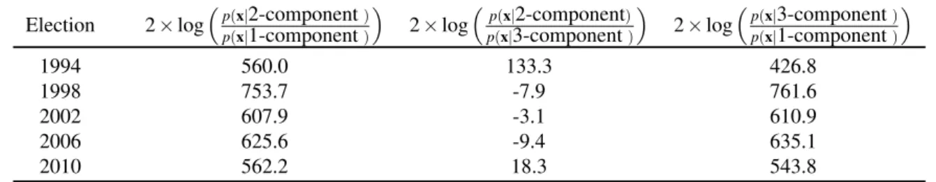
Table 1 –Twice the natural logarithm of the Bayes factor of the data of voting percentage under one model resulting of mixture of Weibull distribution relative to another.

Election 2×logp(_p(x_x|2-component)

|1-component)

2×log_p(p(_xx|2-component)

|3-component)

2×logp(_p(x_x|3-component)

|1-component)

1994 560.0 133.3 426.8

1998 753.7 -7.9 761.6

2002 607.9 -3.1 610.9

2006 625.6 -9.4 635.1

2010 562.2 18.3 543.8

1994

Percentage of votes

Density

0 20 40 60 80

0.00

0.04

0.08

1−component model 2−component model 3−component model

1998

Percentage of votes

Density

0 20 40 60 80

0.00

0.04

0.08

1−component model 2−component model 3−component model

2002

Percentage of votes

Density

0 20 40 60 80

0.00

0.04

0.08

1−component model 2−component model 3−component model

2006

Percentage of votes

Density

0 20 40 60 80

0.00

0.04

0.08

1−component model 2−component model 3−component model

2010

Percentage of votes

Density

0 20 40 60 80

0.00

0.04

0.08

1−component model 2−component model 3−component model

Figure 1 –Histograms of the data of voting percentage obtained by PT in presidential elections, in the cities of

Sergipe State, from year 1994 and 1998, when the PT lost the presidential election, to 2002,2006 and

2010, when the PT candidate was Presidential winner, and its estimated densities based on the posterior predictive distribution for 1, 2 and 3 components.

2.7. Discussion and further development 39

the density for each Model and compare with the histogram of votes as showed in Figure1. We can see that the chosen model, that is the one for which density estimate is closest to the data, coincides with the choice according to Bayes factor.

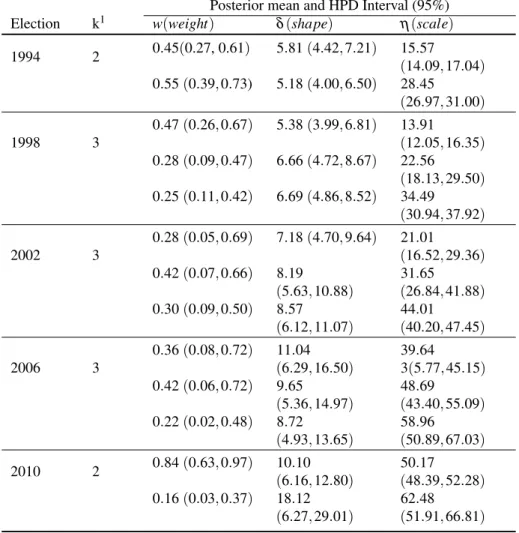
Table2provides posterior means and 95% HPD credible intervals for the parameters in the model chosen according to Bayes factor for each year. The credible intervals were constructed using the package MCMCpackofMartin, Quinn and Park(2011).

Using these parameters we can give some interpretations to the results. For example in 1994 we identified two groups of cities in Sergipe. For the first group, formed by 38 cities and with weight 0.45, we found an expected percentage of votes of 14.4 (posterior mean) with variability of 2.9 (posterior standard deviation), whereas in the second group, formed by 37 cities and with weight 0.55, the corresponding values are higher, 26.2 and 5.8 respectively. Likewise, in 2010, two populations were also identified. For the first population, formed by 67 cities with weight 0.84, we found an expected percentage of votes of 47.8 (posterior mean) with variability of 5.7 (posterior standard deviation), whereas in the second group, formed by 8 cities and with weight 0.16, the corresponding values are higher, 60.7 and 4.1 respectively. Note the significant increment of the percent of votes in both populations between 1994 and 2010. In addition, the first population in 2010 has 33 of the cities in the first group in 1994 indicating specifically that this group of cities had a significant increment over time.

Finally, from the best model for each election, the probability that PT obtains more than 50 percent of the votes in the first round was calculated, because if the presidential candidate won the majority of votes in the first ballot the candidate is declared winner of presidential election and the second ballot is not necessary. The probabilities were estimated considering the predictive distribution by numerical integration using the Simpson rule combined with Monte Carlo method as seen in Section2.5. These corresponding probabilities of winning in the first ballot for PT party considering the Sergipe state for elections in 1994, 1998, 2002, 2006 and 2010 were 3.15_×10−6, 9.76_×10−5, 0.0175, 0.273 and 0.459 respectively, it indicate that this

probability increased over time.

We should note that as suggested by a referee a Mixture Normal model was also imple-mented considering an algorithm similar to the one defined in Section 2.3 without Metropolis-Hastingsstep. The results showed, that there is a strong evidence in favour of the Weibull mixture model. Additionally as discussed in Section 2.1 this model can lead to inferences which can be misleading since the Normal is a symmetric distribution and can lead to over-fit when additional component need to be included to capture the asymmetry in the data.

2.7

Discussion and further development

Table 2 –Posterior mean and HPD interval of parameters of the best Weibull mixture model chosen by Bayes factor evaluation. Data of voting percentage obtained by PT in presidential elections in the Sergipe State from year 1994 to 2010 was considered for fitting of the models.

Posterior mean and HPD Interval (95%)

Election k1 _{w(weight) δ(shape) η(scale)}

1994 2 0.45(0.27, 0.61) 5.81(4.42,7.21) ₍₁₄15.57

.09,17.04) 0.55(0.39,0.73) 5.18(4.00,6.50) 28.45

(26.97,31.00)

1998 3

0.47(0.26,0.67) 5.38(3.99,6.81) 13.91

(12.05,16.35)

0.28(0.09,0.47) 6.66(4.72,8.67) 22.56

(18.13,29.50)

0.25(0.11,0.42) 6.69(4.86,8.52) 34.49

(30.94,37.92)

2002 3

0.28(0.05,0.69) 7.18(4.70,9.64) 21.01

(16.52,29.36)

0.42(0.07,0.66) 8.19

(5.63,10.88)

31.65

(26.84,41.88)

0.30(0.09,0.50) 8.57

(6.12,11.07)

44.01

(40.20,47.45)

2006 3

0.36(0.08,0.72) 11.04

(6.29,16.50)

39.64

3(5.77,45.15) 0.42(0.06,0.72) 9.65

(5.36,14.97)

48.69

(43.40,55.09)

0.22(0.02,0.48) 8.72

(4.93,13.65)

58.96

(50.89,67.03)

2010 2 0.84(0.63,0.97) 10₍₆.10

.16,12.80)

50.17

(48.39,52.28)

0.16(0.03,0.37) 18.12

(6.27,29.01)

62.48

(51.91,66.81)

1_{Number of components in the mixture.}

Brazilian presidential elections from 1994 to 2010 were considered for analysis. A fully Bayesian approach was undertaken using MCMC methods.

We note that the results shown in this paper are purely descriptive. They illustrate how the votes of a particular political party in different elections in Brazil in a given geographic area may exhibit multimodality and how the distribution of votes changes over time. Also, we found that the probability of obtaining 50 percent of the votes in the first ballot is increasing over time.

In future developments, the extension of the analysis for all states of Brazil can be considered as well as regression models for explain the electoral conduct. Since the percentage of votes are limited variables, that is, votes is between a minimum and maximum value, models for limited distributions as Beta distributions also can be explored.

41

CHAPTER

3

MIXTURE OF SIMPLEX DISTRIBUTIONS

WITH UNKNOWN NUMBER OF

COMPONENTS

Abstract

Variables taking values in(0,1), such as rates or proportions, are frequently analyzed by

resear-chers, for instance, political and social data, as well as the Human Development Index. However, sometimes this type of data cannot be modeled adequately using a unique distribution. In this case, we can use mixture of distributions, which is a powerful and flexible probabilistic tool. This manuscript deals with a mixture of Simplex distributions to model proportional data. A fully Bayesian approach is proposed for inference which includes a reversible-jump Markov Chain Monte Carlo procedure. The usefulness of the proposed approach is confirmed by using simulated mixture data from several different scenarios and by using the methodology to analyze municipal Human Development Index data of cities (or towns) in the Northeast region and São Paulo state in Brazil. The analysis shows that among the cities in the Northeast, some appear to have a similar HDI to other cities in São Paulo state.

3.1 Introduction

Variable taking values in (0, 1), such as index and proportions, are frequently analyzed by researchers, for instance Impartial Anonymous Culture (STENSHOLT,1999) and the Human Development Index (HDI) (MCDONALD; RANSOM,2008;CIFUENTESet al.,2008). Someti-mes, the data cannot be modeled adequately using a unique distribution as is the case for the proportion of votes obtained by a political party in the Presidential Elections in each city of a country analyzed in the study conducted byPaz, Bazán and Elher(2015). In addition, different components can be identified in the HDI data of several regions in Brazil, see index inPNUD, IPEA and FJP.(2013).

The mixture models can be a powerful and flexible probabilistic tool for modeling many kinds of data, see for exampleMcLachlan and Peel(2004). In financial data,Faria and Gonçalves(2013), can be cited. In addition, a mixture of distributions has been widely analyzed for Normal data, see for exampleTanner and Wong(1987),Gelfand and Smith(1990),Diebolt and Robert (1994),Richardson and Green (1997). For data in (0,1), there are some studies which consider a finite mixture of Beta distributions (BOUGUILA; ZIOU; MONGA,2006; BOUGUILA; ELGUEBALY,2012). However, other probability distributions with support in the interval (0,1) can be found in the statistics literature, which have not yet been completely analyzed in the context of mixture models, for example the Simplex distribution. The Simplex distribution is a dispersion model proposed byBarndorff-Nielsen and Jorgensen(1991) and has recently been considered as a complementary and alternative regression model when compared to the beta regression model (LÓPEZ,2013;SONG; TAN,2000).

3.2. Simplex Mixture Distribution 43

considers a mixture of Simplex distributions with the number of components unknown (Simplex mixture model). This work is motivated by the municipal HDI data in Brazil. Thus, the aim is to identify the number of components and the characteristics of each population identified by the model considering the HDI of the cities of São Paulo state and the Northeast region of Brazil. In order to deal with the problem of estimating the number of components of the mixture model, a reversible-jump Markov chain Monte Carlo (RJMCMC) approach was adopted (see Green (1995) andRichardson and Green(1997)). A RJMCMC procedure is adopted for the mixture of Simplex distributions with a convenient transition function. The results obtained, considering the proposal, are promising since the performance of the method is tested by applying it to simulated data sets from mixtures of Simplex distributions by considering several different scenarios.

In future developments, it can be considered that the phenomenon can be explained by sociological and economic factors which should be included. In addition, the response variable might be associated to geospatial information as potential covariates.

The remainder of the chapter is organized as follows: In Section 2, the mixture of Simplex distributions is presented. Section 3 addresses the Bayesian inference approach by considering a new estimation RJMCMC method for the mixture of Simplex distributions. Section 4 is dedicated to investigating if our algorithm is able to estimate the mixture parameters and select the number of components considering several scenarios of generated data. In Section 5, an analysis of the municipal HDI data is presented. Finally, some conclusions are drawn in Section 6 and in the ApendiceAwe present a summary of the algorithm used for simulating samples of the jointly posterior distributions of parameters model.

3.2 Simplex Mixture Distribution

Consider initially a sequence ofkcontinuous random variables all taking values in (0,1), each following a distribution with probability density function (pdf)P(._|θj),j=1, . . . ,k. The parameter values inθ1, ...,θk can be different leading to a mixture in the sequence of random variables (r.v.). Then, the pdf of a new r.vY is defined as

P(y_|θθθ,ωωω,k) =

k

∑

j=1

ωjP(y|θj), 0<y<1, (3.1)

where(θθθ,ωωω,k) denotes a vector containing all unknown parameters in the model with θθθ = (θ1, ...,θk),ωωω= (ω1, ...,ωk),ωjis called the mixing proportion satisfyingωj>0 and∑kj=1ωj= 1, andkis the number of components in the mixture, which is assumed unknown.The densities P(._|θj)shall be referred to as the jth component density in the mixture andkas the number of components of the mixture.

In this work, the component densitiesP(._|θj)are taken to belong to the Simplex distribu-tion (JØRGENSEN,1997) whose pdf is given by

S(y_|µ,σ2) =2πσ2(y(1₋y))3−1/2exp

−

₁

2σ2

(y₋µ)2

y(1₋y)µ2(1−µ)2

I_(0,1)(y), (3.2)

where 0<µ<1 is the location parameter andσ2>0 is the dispersion parameter. The mean of the Simplex distribution is given byE(Y) =µ. Since the component densitiesP(._|θj)are assumed to belong to the Simplex distribution family, we shall refer to the component densities in the mixture as Simplex components and the model given by (3.1) as a Simplex Mixture (SM). We shall also rewrite the pdf of this model as

P(y_|θθθ,ωωω,k) =

k

∑

j=1

ωjS(y|θj), 0<y<1, (3.3)

whereθj= (µj,σj2), j=1, ...,k.

3.3 Inference

Considernindependent r.v.Y= (Y1, ..,Yn)of SM model andy= (y1, ..,yn)a realization ofYwhereyiis the observed value of theYi, fori=1, ...,n, then the likelihood corresponding to a SM model with k-component is:

L(θθθ,ωωω,k_|y) =

n

∏

i=1

k

∑

j=1

wjS(yi_|θj).

A way to simplify the inference process of a mixture model is to consider an unobserved random vectorZi= (Zi1, ...,Zik)such thatZi j=1 if theith observation belongs to the jth mixture component andZi j =0 otherwise,i=1, . . . ,n. Note that ∑kj=1Zi j =1, and we suppose each random vectorZ1, ..,Znto be independently distributed according to a multinomial distribution with parameters 1 andωωω = (ω1, ...,ωk) = (P(Zi1=1|ω,k), ...,P(Zik=1|ω,k)), fori=1, ...,n. Then

P(Zi j=1|yi,θj,ω,k)∝P(Zi j =1|ω,k)P(yi|Zi j =1,θj,ω,k) =ωjS(yi|θj),

j =1, ...,k, i=1, . . . ,n. To simplify the notation, we considerZ = (Z₁, ...,Zn)the vector of dimensionnkcontaining all unobserved indicator vectorsZi.

The conditional pdf ofYigivenZiand all parameters can be written as

P(yi|Zi,θθθ,ωωω,k) =P(yi|Zi j=1,θj,ωj,k) =S(yi|θj), for jsuch thatZi j =1. Then the pdf of eachYigivenZiis given by

P(yi|θθθ,Zi,ωωω,k) =S(yi|θj) = k

∏

j=1

S(yi|θj)

Zi j

3.3. Inference 45

Finally, the joint distribution of(Yi,Zi)has the pdf given by

P(yi,Zi|θθθ,ωωω,k) =P(Zi|θθθ,ωωω,k)P(yi|Zi,θθθ,ωωω,k) = k

∏

j=1

ωjS(yi|θj)

Zi j

,i=1, ...,n.

Therefore, after the inclusion of the indicator vectors in the model, the augmented data likelihood to(y,Z)can be written as

L(θθθ,ωωω,k_|y,Z) =

n

∏

i=1

k

∏

j=1

ωjS(yi|θj)

Zi j

. (3.5)

The joint distribution of all variables of the model including the augmented version of the data and the prior specifications is

P(y,θθθ,Z,ωωω,k) =P(y_|θθθ,Z,ωωω,k)P(Z_|ωωω,k)P(θθθ_|Z,ωωω,k)P(ωωω_|k)P(k).

A common approach is to impose conditional independence (BOUGUILA; ELGUEBALY,2012) such thatP(θθθ_|Z,ωωω,k) =P(θθθ_|k),P(y_|θθθ,Z,ωωω,k) =P(y_|θθθ,Z)leading to the joint distribution

P(y,θθθ,Z,ωωω,k) =P(y_|θθθ,Z)P(Z_|ωωω,k)P(θθθ_|k)P(ωωω_|k)P(k), (3.6)

where P(Z_|ωωω,k) = ∏n_i=1P(Zi|ωωω,k) = ∏ni=1

∏k_j=1ωZi j

j

and P(y_|θθθ,Z) =∏_in₌₁P(yi_|θθθ,Zi,ωωω,k)withP(yi_|θθθ,Zi,ωωω,k)given by (3.4).

The mixture model presented here precludes the use of an improper prior. This is because an improper prior leads to an improper posterior, when some of the component become empty. Thus, for the component parameters θj = (µj,σ2j) with φj = σ−j 2,

j=1....k, we choose independent priors, that is,P(θθθ_|Z,ωωω,k) =P(µ/k)P(φ/k)such that µj|k∼U ni f orm(0,1)andφj|k∼Gamma(a,b), j=1, . . . ,k, (3.7) where the hyperparametersaandbare fixed. The scale parameters,µ′_js, are unknown and assume values in the interval(0,1), therefore the unit Uniform seems a good choice for a vague prior. The Gamma distribution with parametersa=b=ε,εbeing a small value, is often chosen as a prior distribution for the precision parameter. In the simulations and the application, we considera=2 andb=1/2 then it is expectedE(φ) =4 andV(φ) =8. Alternative values for hyper-parameters aandbare also used. Considering empirical results, we recommend that the mean and variance of the Gamma prior is in the interval (0,10). ForP(ωωω_|k), since the vector of weightsωωω is defined on

the Simplex

Hence, the full conditional posterior distributions can be obtained, and consequently a Markov chain Monte Carlo method (MCMC) (ROSS,2006, pages, 245 - 271) can be used to sample from the joint probability distribution of the parameters(θθθ,ωωω,k), given the observed

datay,Z. Then the sample of the joint posterior distribution produced by MCMC is used for Bayesian inference.

The full conditional distributions of the parameters for jth components are given by

P(φj|y,Z,µj) ∝ φ

nj/2+a−1

j exp

 



−φj





∑

i∈{i:Zi j=1}

(yi−µj)2

2yi(1−yi)µ2j(1−µj)2

+b      (3.8)

P(µj|y,Z,φj), ∝ exp  



−_2µ2 φj

j(1−µj)2

∑

i_∈{i:Zi j=1}

_(y i−µj)2 yi(1−yi)

 



, (3.9)

wherenj=∑ni=1Zi j denotes the number of observations drawn from a jth component of the

mixture. Note that(φj|y,Z,µj)∼Gamma



nj/2+a,

∑

i∈{i:Zi j=1}

(yi−µj)2

2yi(1−yi)µ2_j(1−µj)2

+b



. In

addition, the full conditional density ofωωω is

P(ωωω_|y,Z)∝

k

∏

j=1

ωνj+nj−1

j , (3.10)

that is the pdf of a Dirichlet distribution, that is,(ωωω_|y,Z)_∼Dirichlet(ν₁+n1, ...,νk+nk)where

ν₁, ...,ν_k are the parameters of the Dirichlet prior. A description of the whole algorithm to

simulate from the joint posterior distribution is given in AppendixAin the end of the thesis. A reversible-jump to estimate the number of components in the mixture is described in the following subsection.

Reversible-jump

Reversible-jump (RJ) MCMC was introduced byGreen(1995) as an extension to MCMC in which the dimension of the model is uncertain.Richardson and Green(1997) extends this method for mixtures of Normal distributions. For the limited data, Bouguila and Elguebaly (2012) develop a procedure to deal with mixtures of beta distributions. However, for mixtures of Simplex distributions, the RJMCMC is not available. In this subsection, we describe a RJMCMC for mixtures of Simplex distributions.

The move in the RJ step, called split-combine moves, allows the increase or reduction of the number of components by one in each step. In each move, the reversible-jump compares two models with different numbers of Simplex components. The split-combine moves form a reversible pair. For this pair, we choose the proposal distributionTk→k* according to informal

considerations in order to obtain a reasonable probability of acceptance. The notationTk_→k*

means the proposal transition function for the move from a model withkSimplex components to a model withk*Simplex components. This move is chosen with probability p_k*_|k. Since the

parametric space of parameters(θθθ,ωωω,k)is different from(θθθ*,ωωω*,k*), the smaller parameter

3.3. Inference 47

complete the parameter space.Green(1995) shows that the balance condition is determined by the acceptance probability to this move given byα((θθθ*,ωωω*,k*)_|(θθθ,ωωω,k)) =min_{1,A_}where

A=L((θθθ

*_,ωωω*_,k*_{)|y,Z)P((θθθ}*_,ωωω*_)|k*_)P(k*_)p

k|k*

L((θθθ,ωωω,k)|y,Z)P((θθθ,ωωω)|k)P(k)p_k*_|kg(u) |J|, (3.11)

whereJis the Jacobian of the transformation. The probability of the inverse move is given by

α((θθθ,ωωω,k)_|(θθθ*,ωωω*,k*)) =min_{1,A−1_}.

The choice between whether to split or combine is made randomly with probabilityb_kand d_k=1₋b_k respectively, depending onk. Note thatd1=0 andbkmax =0 withkmax representing

the maximum value assumed fork, as seen in the previous subsection. If 2<k<kmax we adopt bk=dk=0.5.

If the split move is chosen, we select randomly one component j_* to break into two new components(j1,j2)and create a new state withk*=k+1 components. In order to specify

the new values of parameters for the two components, Richardson and Green(1997) propose generating a vector u= (u1,u2,u3)from beta distributions, and set these parameters using a

deterministic transformation called proposal transition function. This function must be bijective and provide adequate values of parameters. Then, we generateu1∼Beta(2,2),u2∼Beta(1,1)

and u_{3 ∼}Beta(2,2), and in order to set the parameters we propose the proposal transition function such that

ωj1 = ωj*u1, ωj2 = ωj*(1−u1),

µj1 = µj*−u2u1(µj*−µ2j*), µj2 = µj*+u2(1−u1)(µj*−µ2j*),

φ−_j11=σ2_j1 = σ2_j

*u3(1−u

2

2)/u1, φ−j21=σ

2

j2 = σ

2

j_*(1−u3)(1−u22)/(1−u1).

(3.12)

All observations previously allocated to j_*are reallocated doingzi= j1orzi= j2following the

same criteria used in the step (2a) of the Algorithm4.

The combine proposal begins by choosing a pair of components (j1,j2), where the

first is chosen through a discrete Uniform distribution and the second is chosen by making j2 = j1+1, the kth component cannot be chosen in the first place. These two components

are merged, reducingkby 1. The new component is labelled j_*and contains all observations previously allocated to j1and j2doingzi= j*. The parameters for the component j*are set as ωj_* =ωj1+ωj2,µj_* =

µj₁ωj₂+µj₂ωj₁

ωj_* andσ

2

j_* =

σ2_j

2 ω_j 2 ω_j * 

1−

µ_j 2−µj₁

µ_{j* −}µ2_j *

!2



σ2_j 2ωj2 σ2_j

1ωj₁+σ2j₂ωj₂

!. This process is

reversible, i.e., if we first split one component into two and then combine the components j1and

j2, we can recover the previous state. We can also compute the corresponding values ofui’s in the merge move asu1= ω_ωj_j1

*,u2=

µj₂−µj₁ µj_*−µ2j_*

andu3=

ωj₁σ2j₁ ωj₁σ2j₁+ωj₂σ2j₂

.

The acceptance probabilities for split and combine are min_{1,A_}and min_{1,A−1_}respectively, according to (3.11), with

A =

(k+1)





∏

i∈{i:Zi j₁=1}

S(yi|µj1σ

2 j1)



 



∏

i∈{i:Zi j₂=1}

S(yi|µj2σ

2 j2)









∏

i∈{i:Zi j_*=1}

S(yi|µj_*σ2j*)

